Over-Tokenized Transformer: Vocabulary is Generally Worth Scaling

2501.16975

Hongzhi Huang et el.

🤗 2025-01-29

TL;DR
#

Current large language model (LLM) research primarily focuses on scaling model size and training data. However, tokenization, the process of converting text into tokens for model processing, remains less explored in the context of scaling laws. This paper investigates the impact of vocabulary size on LLM performance. Existing research suggests that increasing the vocabulary size can improve performance but also significantly increases the training cost. This paper aims to improve this area by focusing on efficient model scaling while considering vocabulary size as a critical factor.

This research introduces Over-Tokenized Transformers, a novel framework that decouples input and output vocabularies to improve model scalability. The researchers discover that scaling up the input vocabulary size leads to a log-linear relationship between input vocabulary size and training loss. This means that using a larger input vocabulary consistently improves model performance. They achieve performance comparable to using double-sized baselines with no extra cost. The findings highlight the importance of tokenization in scaling laws and suggest new approaches for tokenizer design.

Key Takeaways
#

Why does it matter?
#

This paper is crucial because it challenges conventional wisdom in large language model (LLM) development. By demonstrating the significant impact of tokenization on model scaling and performance, it opens new avenues for research and development of more efficient and powerful LLMs. The findings are particularly relevant given the current focus on scaling laws and the ongoing quest for better LLM performance. Researchers can leverage this work to improve LLM design and training efficiency, leading to advancements in the field.

Visual Insights
#

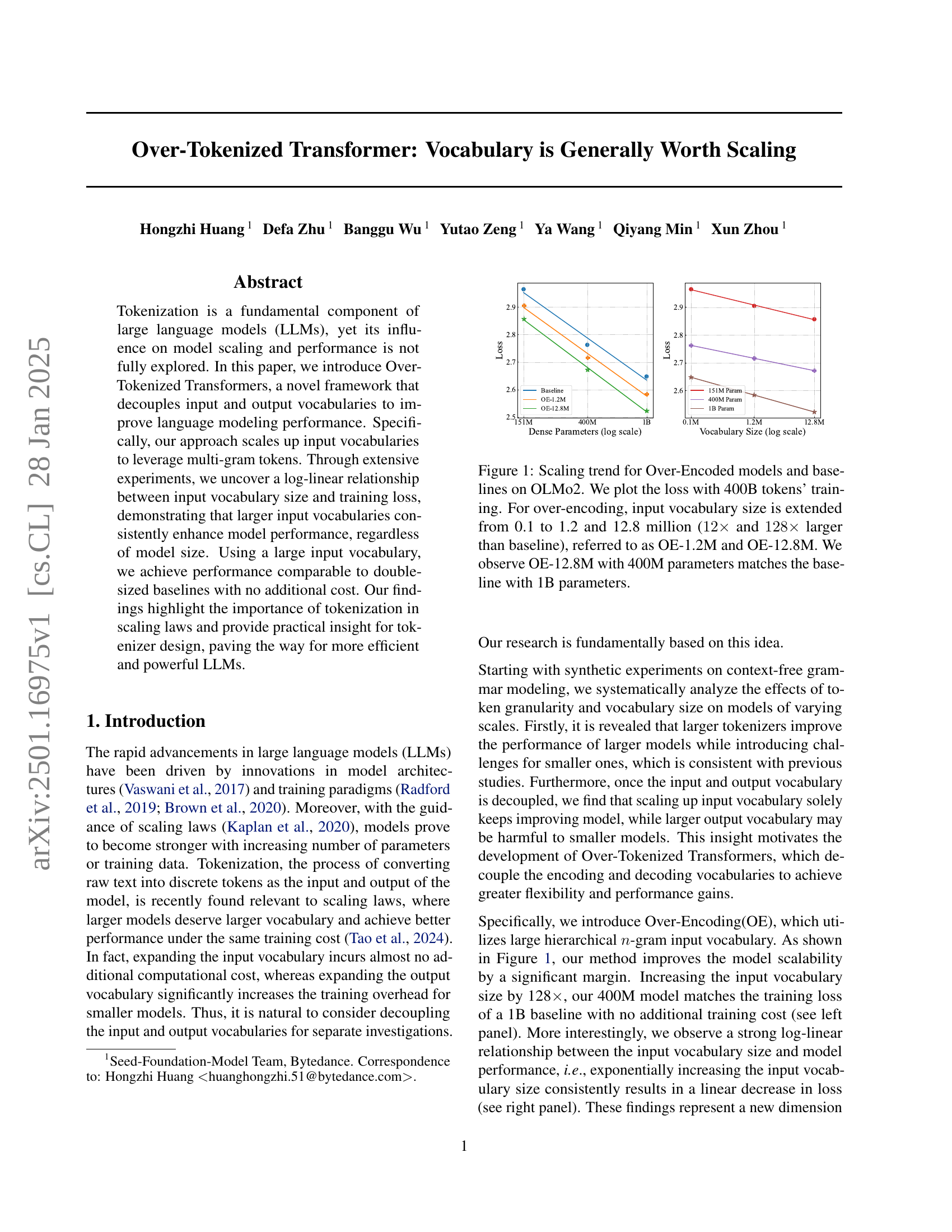
🔼 This figure displays the scaling trend of Over-Encoded (OE) models compared to baseline models on the OLMo2 dataset. The x-axis represents the number of dense parameters (log scale), while the y-axis shows the training loss. Four lines are plotted: a baseline model and three OE models. The baseline model’s loss is shown for models with 151 million, 400 million, and 1 billion parameters. The three OE models represent different increases in input vocabulary size compared to the baseline: OE-1.2M (12x larger), and OE-12.8M (128x larger). The training data used to generate these results included 400 billion tokens. Notably, the OE-12.8M model with 400 million parameters achieves a loss comparable to that of the baseline model with 1 billion parameters, demonstrating the effect of increased input vocabulary size on model performance.
read the caption
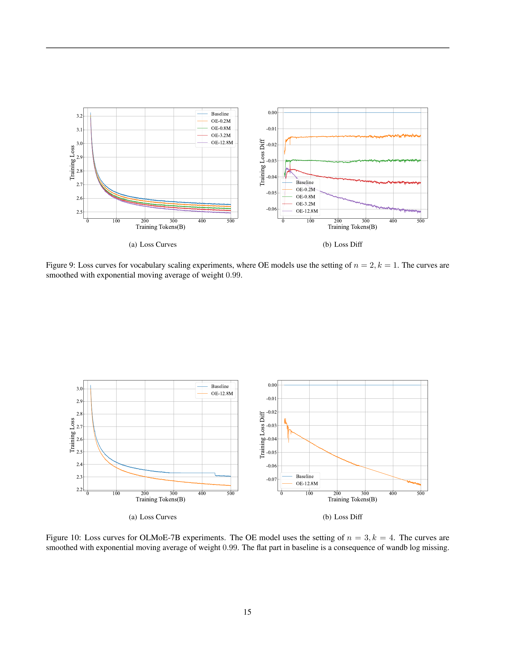
Figure 1: Scaling trend for Over-Encoded models and baselines on OLMo2. We plot the loss with 400B tokens’ training. For over-encoding, input vocabulary size is extended from 0.1 to 1.2 and 12.8 million (12×12\times12 × and 128×128\times128 × larger than baseline), referred to as OE-1.2M and OE-12.8M. We observe OE-12.8M with 400M parameters matches the baseline with 1B parameters.

Model	# Emb. P.	Loss $\downarrow$	Downstream $\uparrow$
OLMoE-1.3B	51M	2.554	0.510
+OE-12.8M	13.1B	2.472 -0.082	0.524 +0.014
OLMoE-7B	102M	2.305	0.601
+OE-12.8M	26.3B	2.229 -0.076	0.608 +0.007

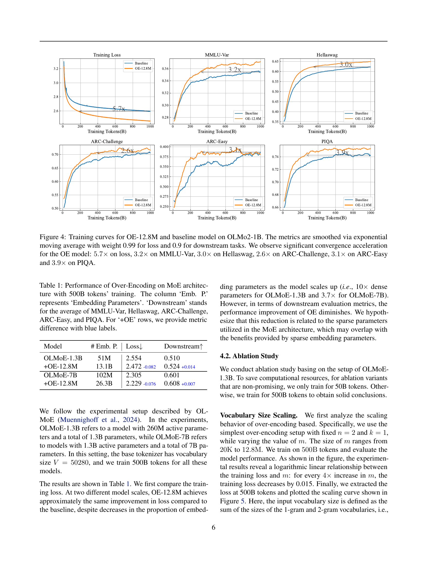
🔼 This table presents the results of experiments evaluating the impact of Over-Encoding (OE) on Mixture-of-Experts (MoE) models. Models were trained with 500 billion tokens. The table compares baseline MoE models (OLMOE) with OE-enhanced versions. Key metrics include training loss, downstream task performance (averaged across MMLU-Var, Hellaswag, ARC-Challenge, ARC-Easy, and PIQA), and the number of embedding parameters. For each OE model, the improvement in the downstream tasks and loss compared to the baseline is highlighted in blue.
read the caption
Table 1: Performance of Over-Encoding on MoE architecture with 500B tokens’ training. The column ‘Emb. P.’ represents ‘Embedding Parameters’. ‘Downstream’ stands for the average of MMLU-Var, Hellaswag, ARC-Challenge, ARC-Easy, and PIQA. For ‘+OE’ rows, we provide metric difference with blue labels.

In-depth insights
#

Vocab Scaling Laws
#

The concept of “Vocab Scaling Laws” in the context of large language models (LLMs) explores the relationship between vocabulary size and model performance. Intuitively, a larger vocabulary allows the model to capture more nuanced linguistic information, leading to improved performance. However, simply increasing vocabulary size isn’t a straightforward solution. The paper investigates this complex relationship, uncovering a log-linear relationship between input vocabulary size and training loss. This means that increasing the input vocabulary size exponentially results in a linearly decreasing training loss, suggesting significant potential gains from carefully scaling the vocabulary. However, the impact of expanding output vocabulary is less clear and might even negatively impact smaller models, highlighting the need for decoupling input and output vocabulary scaling strategies for optimal performance. The authors propose “Over-Tokenized Transformers,” a novel framework to leverage these scaling laws, emphasizing the importance of tokenizer design as a critical factor in building more efficient and powerful LLMs. Further research into this area could uncover even more refined strategies for vocabulary scaling and unlock new advancements in LLM architecture and efficiency.

Over-Tokenization
#

The concept of ‘over-tokenization’ challenges conventional approaches to tokenization in large language models (LLMs). Instead of relying on standard tokenizers that produce a fixed vocabulary size, over-tokenization explores the benefits of significantly expanding the input vocabulary, often using n-grams (sequences of multiple words). This decoupling of input and output vocabularies allows the model to capture richer contextual information, potentially improving performance, especially for larger models. However, simply increasing the output vocabulary size isn’t always beneficial, particularly for smaller models, as it can lead to overfitting or increased computational costs. The research highlights a log-linear relationship between input vocabulary size and training loss, suggesting that larger input vocabularies consistently lead to performance improvements. Efficient techniques are crucial for managing the computational challenges of very large vocabularies, such as hierarchical encoding and tensor parallelism, which are essential to make over-tokenization practical. Overall, the findings demonstrate that vocabulary scaling is a significant factor in LLM performance and that carefully considered over-tokenization strategies can lead to more efficient and powerful models.

OE/OD Decoupling
#

The core idea of “OE/OD Decoupling” revolves around separating the input (Over-Encoding or OE) and output (Over-Decoding or OD) vocabulary scaling processes in transformer models. Traditionally, both input and output vocabularies are tightly coupled, often increasing in size simultaneously. This paper argues that this approach is suboptimal, as scaling up the output vocabulary leads to significantly higher computational costs, particularly for smaller models. Decoupling allows for independent optimization of input and output vocabularies, leveraging the benefits of a larger input vocabulary (OE) which enhances model representation without incurring the cost of a similarly sized output vocabulary. The findings strongly suggest that scaling up the input vocabulary alone (OE) consistently improves model performance and scaling efficiency, regardless of model size, while scaling up the output vocabulary (OD) might prove detrimental to smaller models. This decoupling technique opens a new path towards creating more efficient and powerful LLMs, offering a new dimension for model scaling exploration, and highlights the previously under-appreciated importance of tokenization in overall model architecture and scaling laws.

Engineering OE
#

Engineering efficient Over-Encoding (OE) is crucial for practical application. The core challenge lies in handling the massive input vocabulary generated by n-gram tokenization. Naive implementations would lead to impractically large embedding tables, exceeding available GPU memory. The authors cleverly address this by proposing a tiled matrix parameterization approach. This method cleverly maps the vast n-gram vocabulary onto a smaller embedding table through a modulo operation, significantly reducing memory footprint. Furthermore, they introduce hierarchical encoding, combining 1-gram and n-gram embeddings to boost performance while managing costs effectively. Tensor parallelism is strategically leveraged to optimize communication overhead during training, especially crucial when using distributed training frameworks like FSDP. The effectiveness of this engineering is demonstrated by the close performance match between the larger baseline model and the significantly smaller OE model, showcasing the potential for enhancing model scalability and efficiency. Addressing memory and communication bottlenecks via smart engineering is critical for making this approach viable.

Future of Tokenization
#

The future of tokenization in large language models (LLMs) is likely to be characterized by a move towards more sophisticated and adaptable methods. Beyond simple byte-pair encoding (BPE) or unigram language models, we can expect to see a rise in techniques that leverage the strengths of various approaches. This might involve hybrid models combining subword tokenization with character-level or word-level approaches, depending on the specific needs of the model and the data it is trained on. We might also see increased use of adaptive tokenization, where the tokenizer is trained alongside the model and adjusts its strategy based on the model’s performance. Another promising direction is the exploration of tokenization methods that go beyond simple segmentation, such as those that incorporate information about word morphology, syntax, or semantics. These advancements would enable LLMs to achieve a better understanding of language structure and context, leading to significant performance improvements. Furthermore, research in efficient and scalable tokenization for extremely large models is crucial. This could involve exploring techniques to reduce the computational cost of tokenization or the memory footprint of vocabulary embeddings. The future of tokenization is inextricably linked to the overall advancement of LLMs, and its continued evolution will be instrumental in unlocking even more powerful and efficient models.

More visual insights
#

More on figures

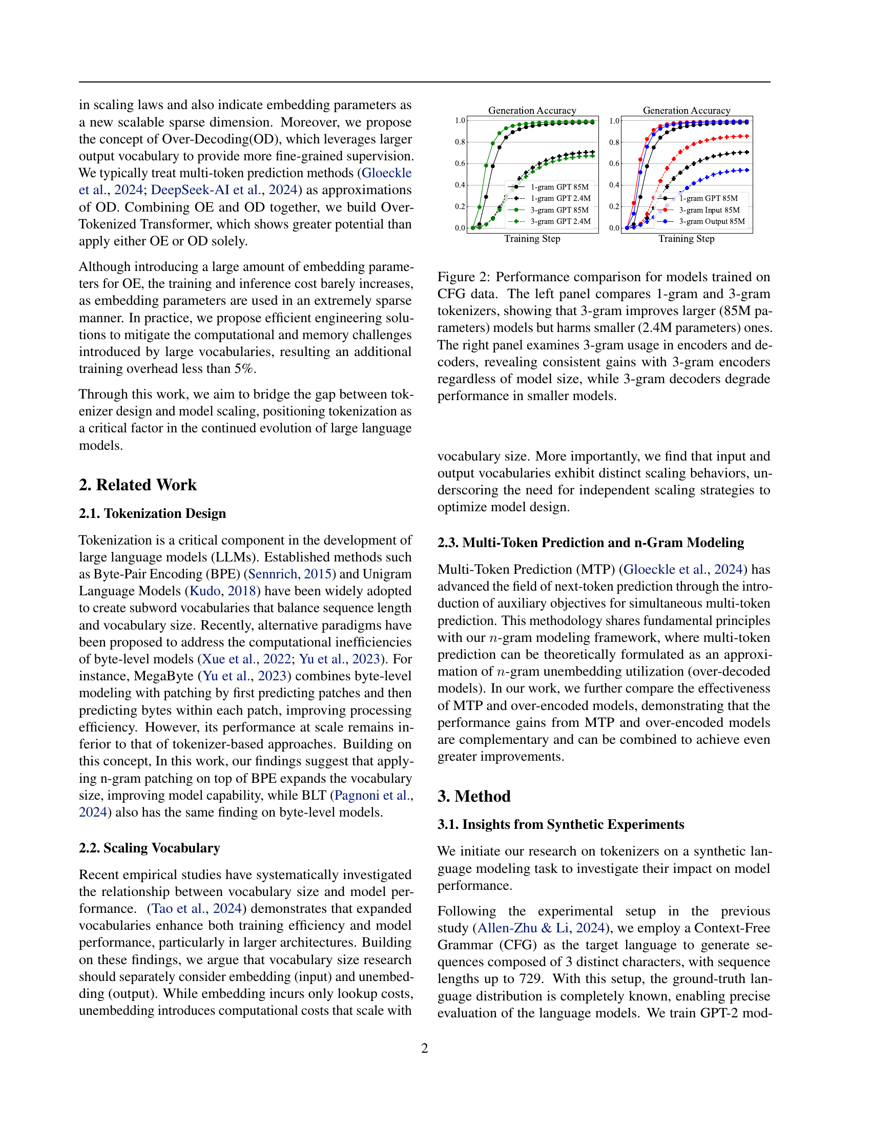
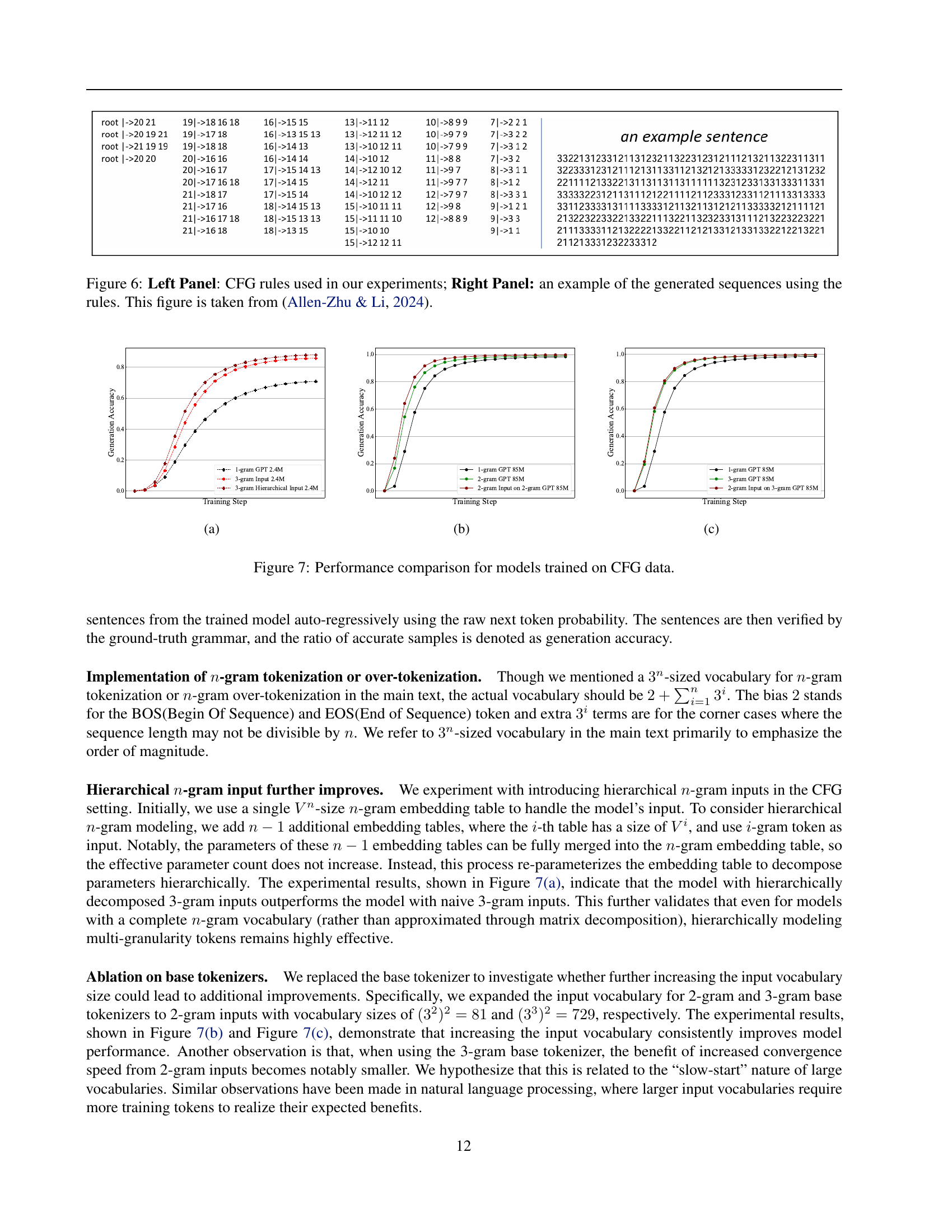
🔼 This figure displays the results of experiments comparing the performance of language models trained on context-free grammar (CFG) data using different tokenization strategies. The left panel shows that using 3-gram tokenizers (which consider groups of three consecutive characters) improves the performance of larger language models (85 million parameters) compared to 1-gram tokenizers (considering single characters), but it harms smaller models (2.4 million parameters). This suggests that larger models benefit from the richer information captured by 3-gram tokens, while smaller models might be over-burdened by the increased complexity. The right panel investigates the impact of 3-gram tokenization on encoders (input processing) and decoders (output generation) separately. The results reveal consistent performance improvements when using 3-gram encoders, regardless of the model’s size. However, 3-gram decoders hurt the performance of smaller models, highlighting the importance of considering the model size when designing tokenization strategies.
read the caption
Figure 2: Performance comparison for models trained on CFG data. The left panel compares 1-gram and 3-gram tokenizers, showing that 3-gram improves larger (85M parameters) models but harms smaller (2.4M parameters) ones. The right panel examines 3-gram usage in encoders and decoders, revealing consistent gains with 3-gram encoders regardless of model size, while 3-gram decoders degrade performance in smaller models.

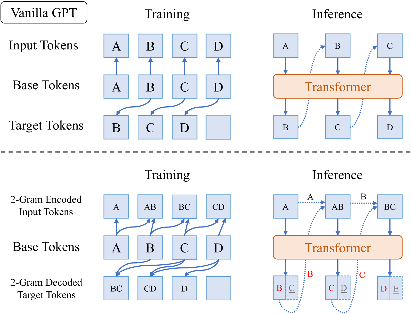
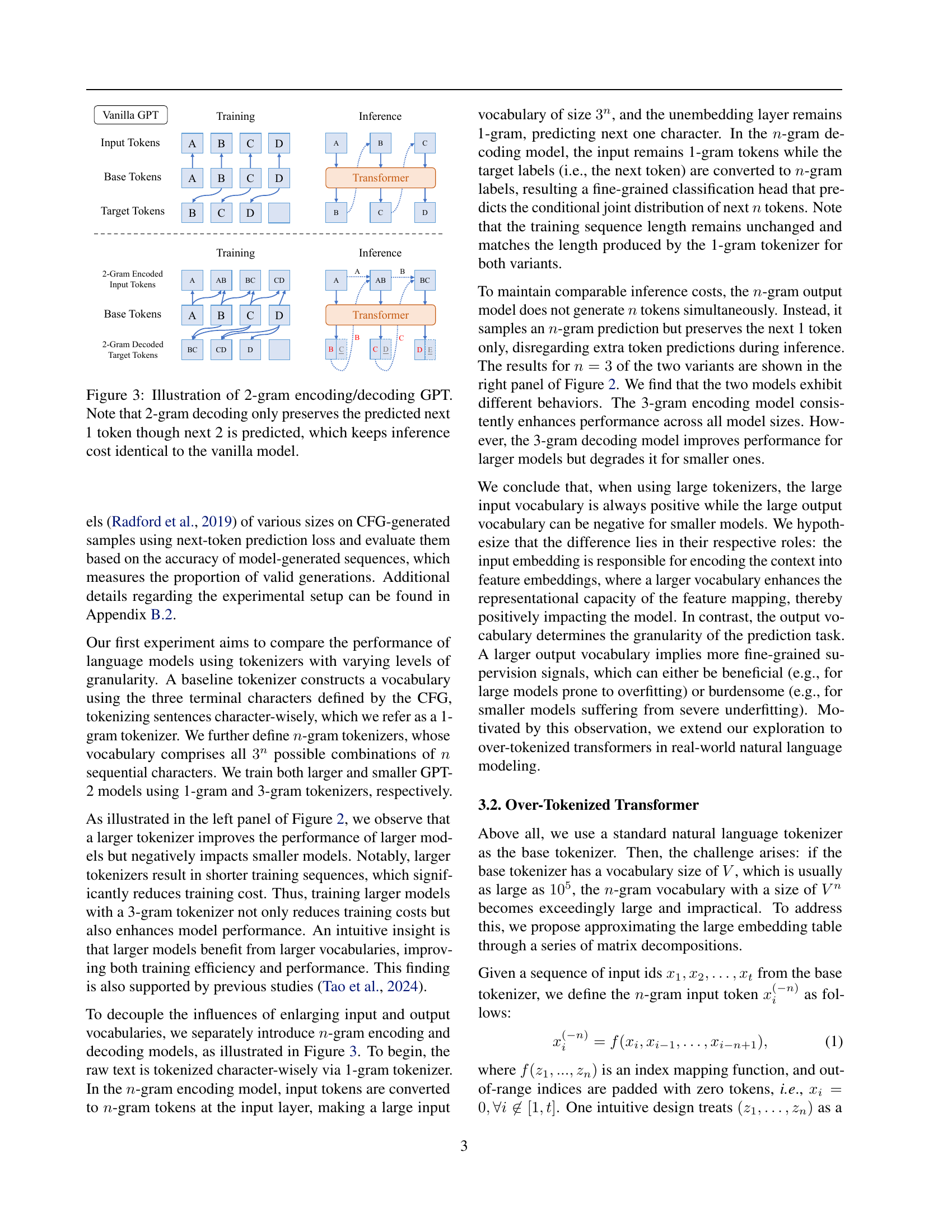
🔼 This figure illustrates the difference between a standard GPT (Vanilla GPT) and a GPT model using 2-gram encoding and decoding. In Vanilla GPT, both input and output tokens are single units (1-gram). In the 2-gram encoding GPT, the input is encoded as 2-grams (sequences of two consecutive tokens), allowing the model to learn relationships between adjacent tokens. However, the output (prediction) remains 1-gram to maintain a similar inference cost as Vanilla GPT. The 2-gram decoding GPT works inversely. The input remains a 1-gram but the output is a 2-gram prediction. It shows that the 2-gram encoding captures local context, and the 2-gram decoding provides finer-grained supervision signals.
read the caption
Figure 3: Illustration of 2-gram encoding/decoding GPT. Note that 2-gram decoding only preserves the predicted next 1 token though next 2 is predicted, which keeps inference cost identical to the vanilla model.

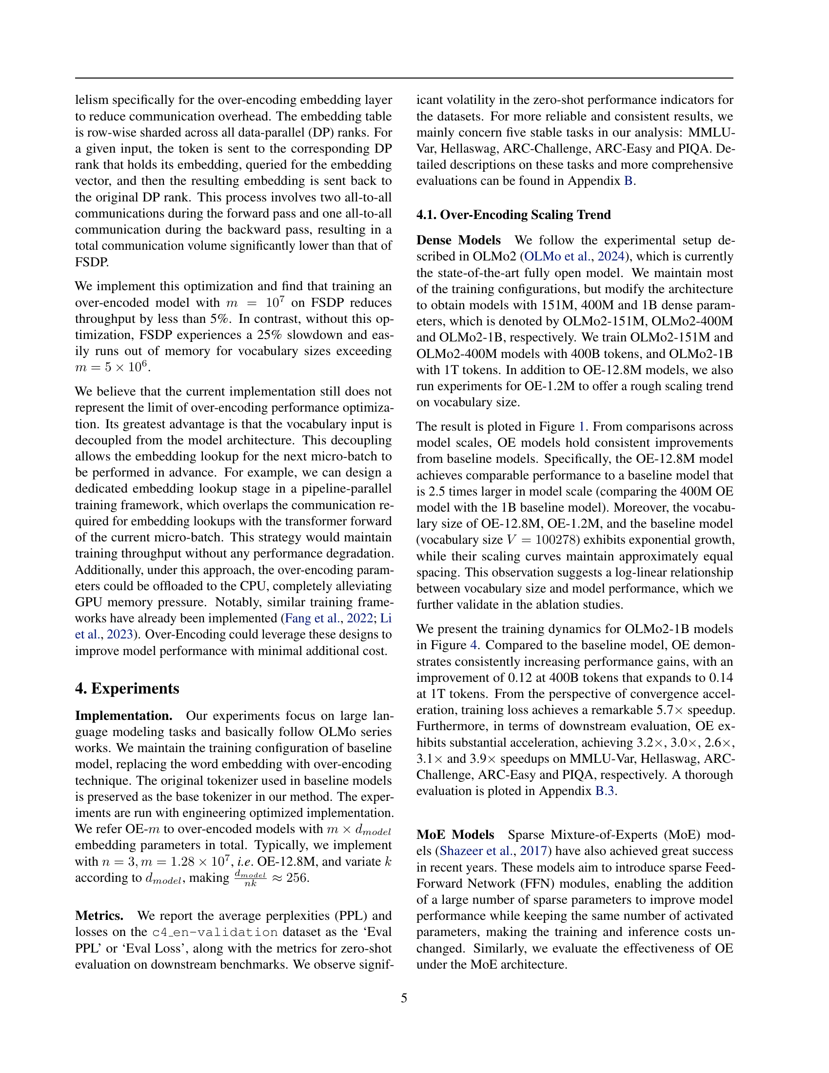
🔼 Figure 4 presents a detailed comparison of training curves between the baseline OLMo2-1B model and the over-encoded model (OE-12.8M) which uses a significantly larger input vocabulary. The comparison includes training loss and zero-shot performance on several downstream tasks: MMLU-Var, Hellaswag, ARC-Challenge, ARC-Easy, and PIQA. Exponential moving averages (EMA) were applied for smoothing the curves (0.99 for loss and 0.9 for downstream metrics). The results show a dramatic speedup in convergence for the OE-12.8M model, achieving 5.7x faster convergence in loss compared to the baseline. Substantial improvements are also observed in the downstream task scores (3.2x on MMLU-Var, 3x on Hellaswag, 2.6x on ARC-Challenge, 3.1x on ARC-Easy, and 3.9x on PIQA). This demonstrates the substantial performance gains enabled by increasing the input vocabulary size.
read the caption
Figure 4: Training curves for OE-12.8M and baseline model on OLMo2-1B. The metrics are smoothed via exponential moving average with weight 0.99 for loss and 0.9 for downstream tasks. We observe significant convergence acceleration for the OE model: 5.7×5.7\times5.7 × on loss, 3.2×3.2\times3.2 × on MMLU-Var, 3.0×3.0\times3.0 × on Hellaswag, 2.6×2.6\times2.6 × on ARC-Challenge, 3.1×3.1\times3.1 × on ARC-Easy and 3.9×3.9\times3.9 × on PIQA.

🔼 This figure displays the log-linear relationship between the input vocabulary size (m) and the training loss (L) observed during experiments. Specifically, it shows that as the logarithm of the vocabulary size increases linearly, the training loss decreases linearly. This relationship was determined using 500 billion tokens of training data on the OLMoE-1.3B model. The equation representing this relationship is provided: L = 2.6754 - 0.0256 * log₁₀(m).
read the caption
Figure 5: Log-linear relationship is observed between vocabulary size m𝑚mitalic_m and training loss ℒℒ\mathcal{L}caligraphic_L, i.e. ℒ=2.6754−0.0256×log10⁡mℒ2.67540.0256subscript10𝑚\mathcal{L}=2.6754-0.0256\times\log_{10}{m}caligraphic_L = 2.6754 - 0.0256 × roman_log start_POSTSUBSCRIPT 10 end_POSTSUBSCRIPT italic_m. The values are collected with 500B tokens’ training on OLMoE-1.3B models.

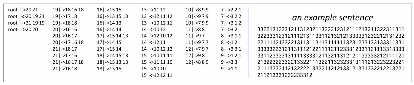
🔼 This figure is from Allen-Zhu & Li (2024). The left panel shows the context-free grammar (CFG) rules used to generate synthetic data for the experiments in the paper. The rules define the relationships between different symbols in the language. The right panel displays an example of a sequence generated using these rules. This sequence is a string of characters created according to the grammatical rules defined on the left.
read the caption
Figure 6: Left Panel: CFG rules used in our experiments; Right Panel: an example of the generated sequences using the rules. This figure is taken from (Allen-Zhu & Li, 2024).

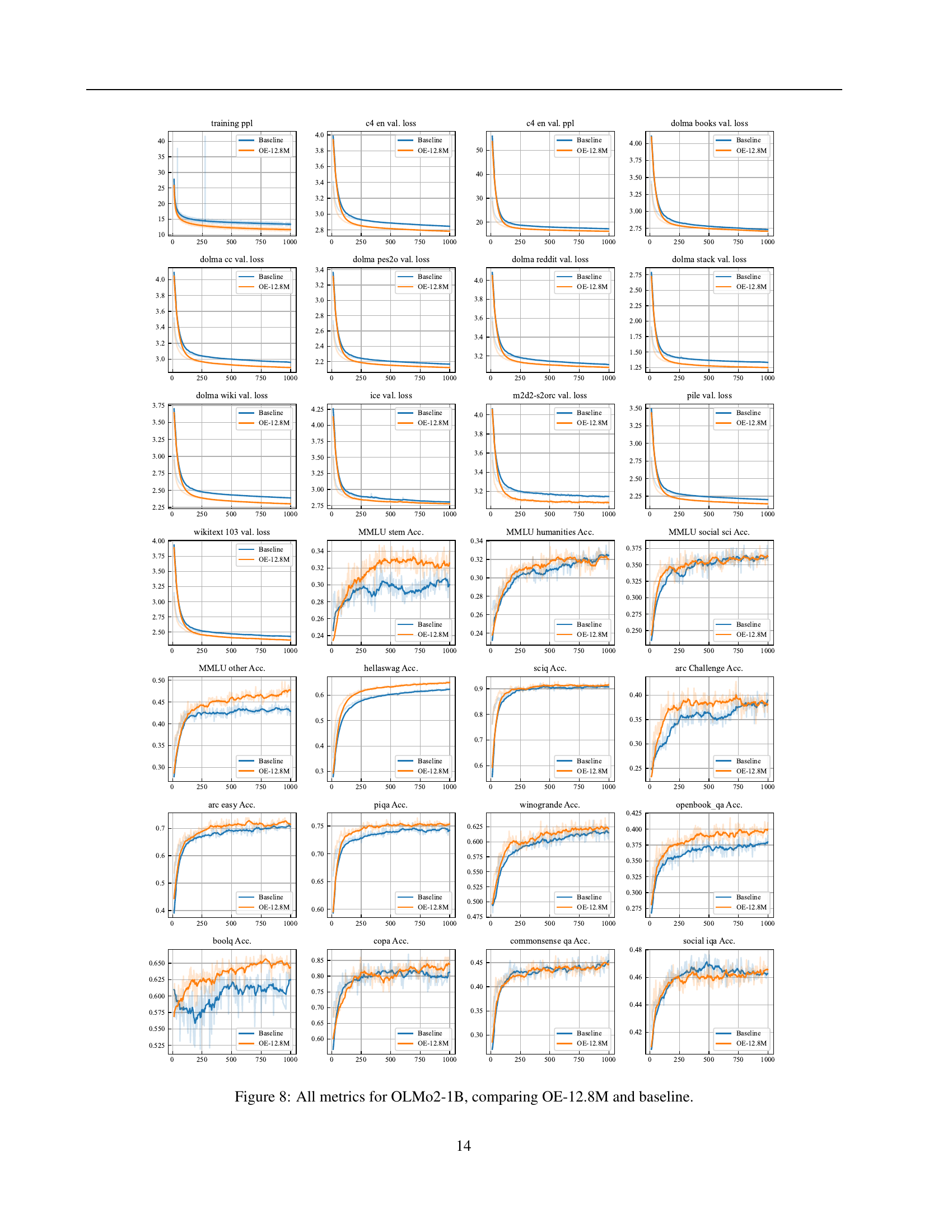
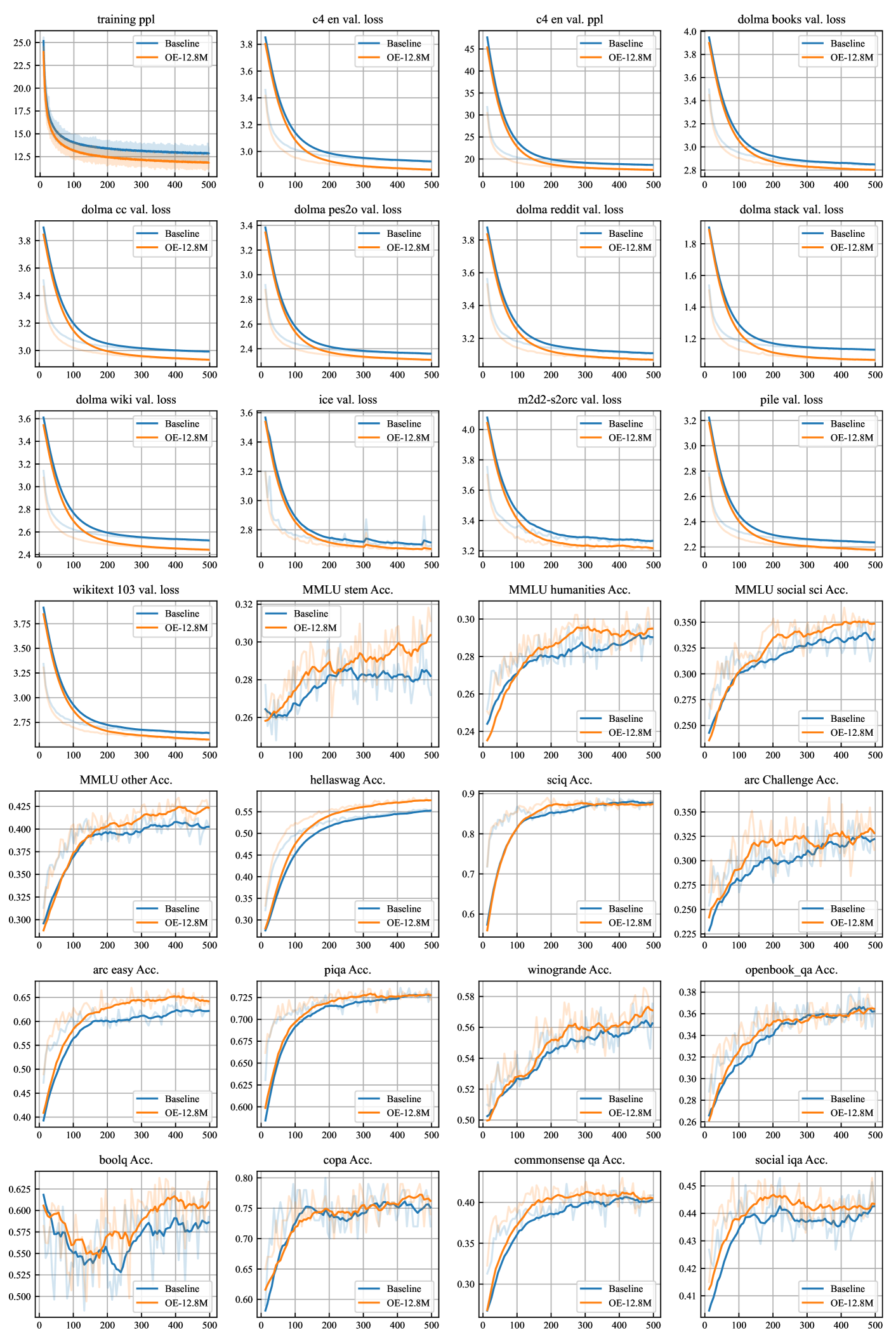
🔼 This figure displays a comprehensive comparison of various metrics between the baseline OLMo2-1B model and the OLMo2-1B model enhanced with Over-Encoding (OE-12.8M). Metrics include training loss and perplexity, as well as several downstream task evaluation metrics, such as performance on the MMLU, HellaSwag, ARC (Challenge and Easy), PIQA, BoolQ, COPA, CommonsenseQA, and Social-IQA benchmarks. The visualization allows for a direct assessment of how Over-Encoding impacts both training dynamics and overall model performance across a range of tasks. Each metric’s trend is shown over the course of training, providing insights into convergence speed and final performance.
read the caption
Figure 9: All metrics for OLMo2-1B, comparing OE-12.8M and baseline.

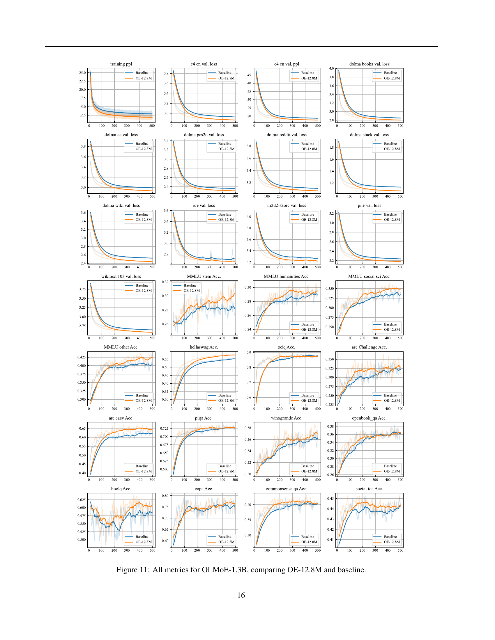
🔼 Figure 11 presents a comprehensive comparison of various performance metrics between the OLMoE-1.3B model with over-encoding (OE-12.8M) and its baseline counterpart. The metrics encompass training loss, validation loss, perplexity scores on several datasets (C4-en, Dolma Books, etc.), and zero-shot performance across numerous downstream tasks (e.g., MMLU-Var, HellaSwag, ARC-Challenge, ARC-Easy, PIQA, etc.). The figure visually depicts the training dynamics and final evaluation scores, offering a detailed assessment of how OE-12.8M impacts both model training efficiency and overall performance across various benchmarks.
read the caption
Figure 11: All metrics for OLMoE-1.3B, comparing OE-12.8M and baseline.

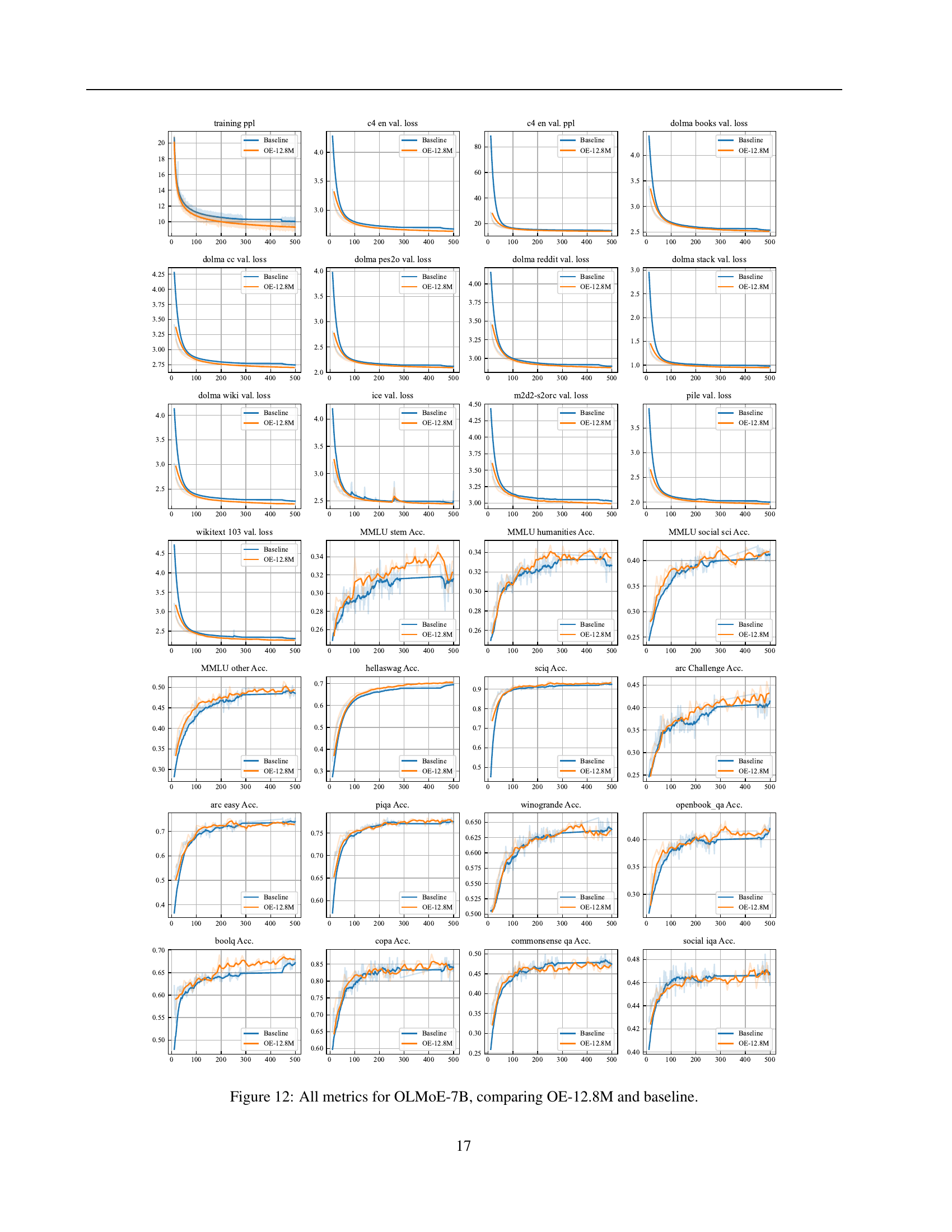
🔼 This figure presents a comprehensive comparison of various metrics for the OLMoE-7B model with and without over-encoding (OE-12.8M). Metrics include training loss and perplexity, as well as downstream task performance across several benchmarks like MMLU (various sub-categories), HellaSwag, SciTail, ARC (Challenge and Easy), PIQA, Winogrande, BoolQ, COPA, CommonsenseQA, and SocialIQA. Each metric is shown over the course of the training process, illustrating the impact of over-encoding on both training dynamics and final performance across a range of tasks.
read the caption
Figure 12: All metrics for OLMoE-7B, comparing OE-12.8M and baseline.

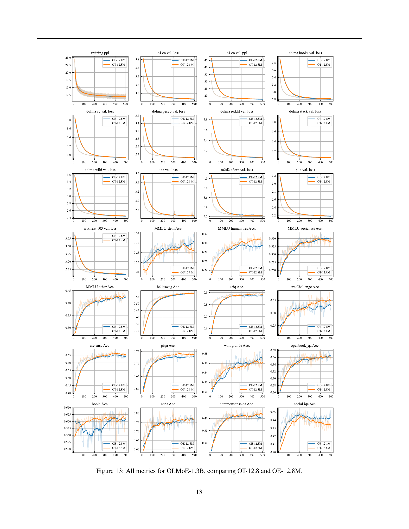
🔼 Figure 13 presents a comprehensive comparison of various evaluation metrics for the OLMoE-1.3B model, contrasting the performance achieved using Over-Tokenized Transformers (OT-12.8M) against that of Over-Encoded Transformers (OE-12.8M). The metrics cover a wide range, including training loss, perplexity, and various downstream benchmark scores across diverse tasks like MMLU (covering STEM, humanities, and social sciences), HellaSwag, ARC (easy and challenge), PIQA, Winogrande, BoolQ, COPA, CommonsenseQA, and SocialIQA. This detailed visualization allows readers to directly assess the impact of integrating over-decoding with over-encoding, facilitating a comprehensive understanding of the relative strengths and weaknesses of each approach in a large language model setting.
read the caption
Figure 13: All metrics for OLMoE-1.3B, comparing OT-12.8 and OE-12.8M.

More on tables

Id	Model	Train		Eval		Downstream
Id	Model	Loss $\downarrow$	PPL $\downarrow$	Loss $\downarrow$	PPL $\downarrow$	MMLU-V $\uparrow$	HS $\uparrow$	ARC-C $\uparrow$	ARC-E $\uparrow$	PIQA $\uparrow$
1	OLMoE-1.3B	2.554	12.864	2.924	18.625	0.327	0.553	0.325	0.622	0.727
2	+ $\mathbb{E}^{3.2\mathrm{M}\times d}(x^{(-2)})$	2.511	12.319	2.887	17.944	0.340	0.569	0.351	0.656	0.734
3	+ $\mathbb{E}^{6.4\mathrm{M}\times\frac{d}{2}}(x^{(-2)})$	2.507	12.268	2.882	17.851	0.330	0.573	0.341	0.648	0.731
4	+ $\mathbb{E}^{3.2\mathrm{M}\times d\|2}(x^{(-2)})$	2.503	12.221	2.877	17.754	0.337	0.575	0.345	0.651	0.740
5	+ $\mathbb{E}^{3.2\mathrm{M}\times d\|4}(x^{(-2)})$	2.503	12.226	2.876	17.736	0.328	0.575	0.337	0.653	0.734
6	+ $\sum_{i\in\{2,3\}}\mathbb{E}_{i}^{3.2\mathrm{M}\times\frac{d}{2}\|2}(x^{(-i)})$	2.495	12.127	2.870	17.638	0.340	0.578	0.330	0.636	0.738
7	+ $\mathbb{E}^{12.8\mathrm{M}\times d}(x^{(-2)})$	2.493	12.100	2.881	17.832	0.334	0.569	0.343	0.643	0.730
8	+ $\sum_{i\in\{2,3\}}\mathbb{E}_{i}^{12.8\mathrm{M}\times\frac{d}{2}\|2}(x^{(-i)})$	2.472	11.854	2.862	17.494	0.342	0.577	0.329	0.645	0.728

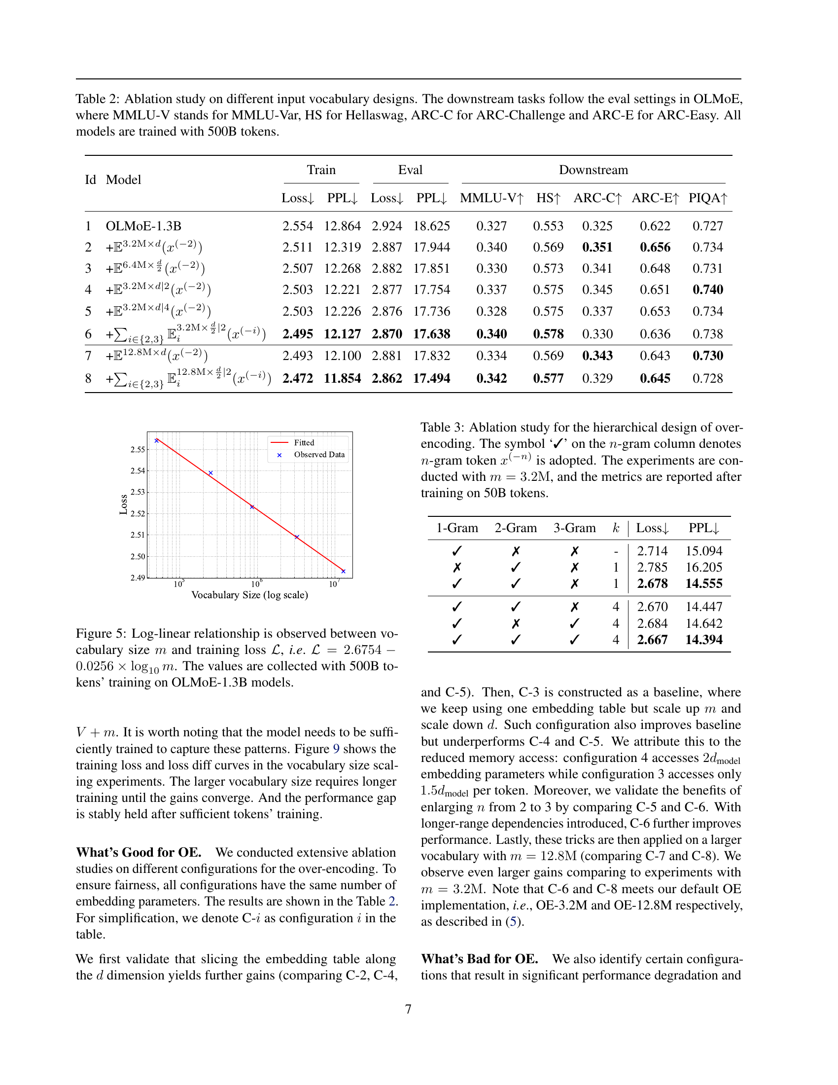
🔼 This table presents an ablation study analyzing the impact of various input vocabulary designs on model performance. It compares different configurations of over-encoding, varying the size and structure of the input vocabulary (n-grams and embedding dimensions). The results are evaluated using training loss, perplexity, and multiple downstream benchmark tasks (MMLU-Var, Hellaswag, ARC-Challenge, ARC-Easy, and PIQA), each designed to measure specific aspects of language understanding. All models in the study were trained with 500 billion tokens to ensure sufficient training.
read the caption
Table 2: Ablation study on different input vocabulary designs. The downstream tasks follow the eval settings in OLMoE, where MMLU-V stands for MMLU-Var, HS for Hellaswag, ARC-C for ARC-Challenge and ARC-E for ARC-Easy. All models are trained with 500B tokens.

1-Gram	2-Gram	3-Gram	$k$	Loss $\downarrow$	PPL $\downarrow$
✓	✗	✗	-	2.714	15.094
✗	✓	✗	1	2.785	16.205
✓	✓	✗	1	2.678	14.555
✓	✓	✗	4	2.670	14.447
✓	✗	✓	4	2.684	14.642
✓	✓	✓	4	2.667	14.394

🔼 This table presents an ablation study on the hierarchical design of over-encoding in the context of natural language processing. It investigates the impact of different combinations of 1-gram, 2-gram, and 3-gram tokens on model performance. The study uses a fixed embedding size (m=3.2M) and trains the model with 50 billion tokens. The results, including training loss and perplexity, are compared across different configurations to determine the optimal approach for incorporating hierarchical input tokens in over-encoding models.
read the caption
Table 3: Ablation study for the hierarchical design of over-encoding. The symbol ‘✓’ on the n𝑛nitalic_n-gram column denotes n𝑛nitalic_n-gram token x(−n)superscript𝑥𝑛x^{(-n)}italic_x start_POSTSUPERSCRIPT ( - italic_n ) end_POSTSUPERSCRIPT is adopted. The experiments are conducted with m=3.2⁢M𝑚3.2Mm=3.2\mathrm{M}italic_m = 3.2 roman_M, and the metrics are reported after training on 50B tokens.

Model	Loss $\downarrow$	PPL $\downarrow$	Eval Loss $\downarrow$	Eval PPL $\downarrow$
baseline	2.714	15.094	3.094	22.060
+ $\mathbb{E}^{64V\times d}$	2.702	14.892	3.077	21.710
+ $\mathbb{E}^{3.2\mathrm{M}\times d}$	2.678	14.555	3.054	21.202

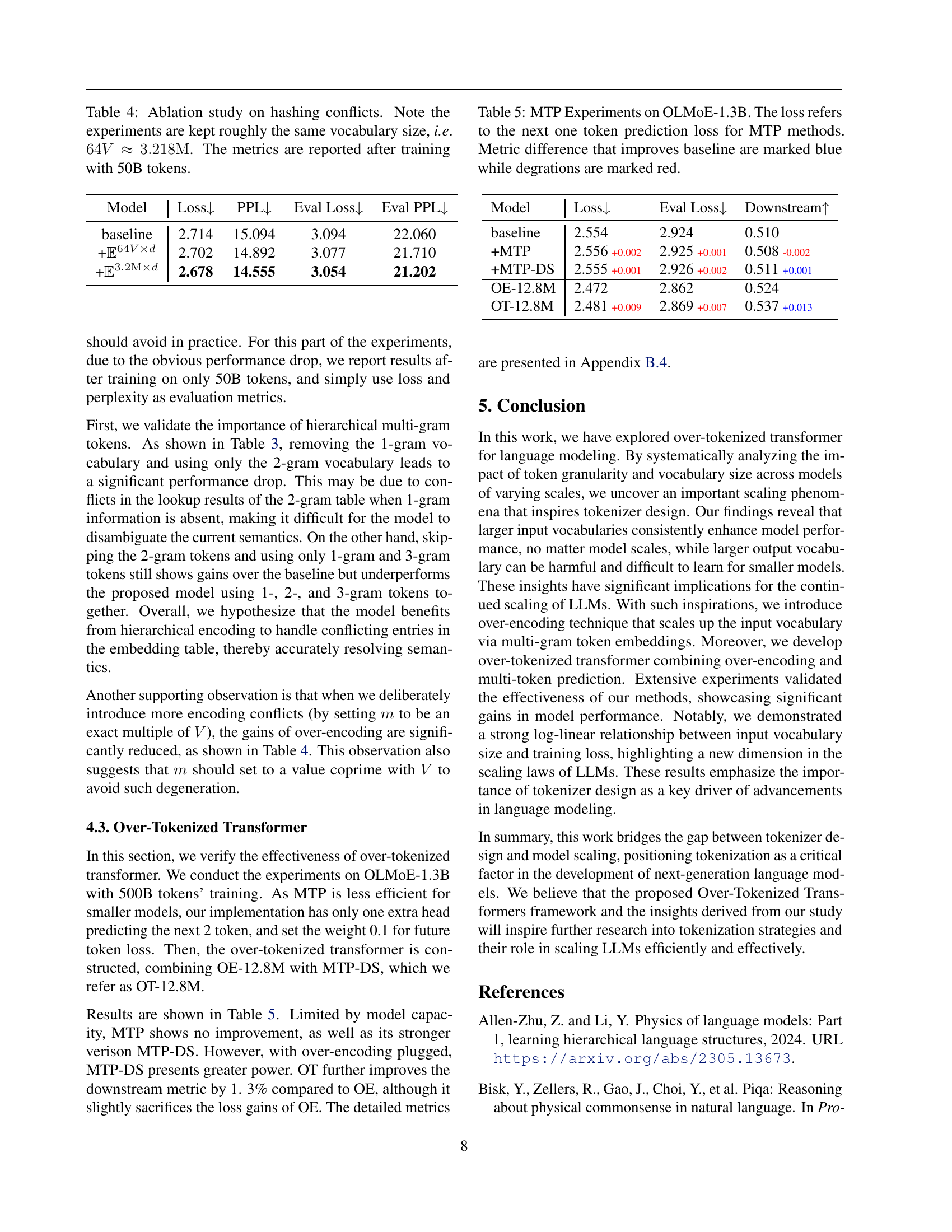
🔼 This ablation study investigates the impact of hashing collisions in the over-encoding method on model performance. It compares several model configurations with approximately the same vocabulary size (~3.2M), varying the way input tokens are mapped to embeddings, to isolate the effects of hashing conflicts. All models were trained with 50B tokens, and the results (training loss, evaluation loss, and downstream task performance metrics) are reported to assess the impact of different embedding strategies. The goal is to determine the best strategy for minimizing the negative effects of hashing collisions on the effectiveness of over-encoding.
read the caption
Table 4: Ablation study on hashing conflicts. Note the experiments are kept roughly the same vocabulary size, i.e. 64⁢V≈3.218⁢M64𝑉3.218M64V\approx 3.218\mathrm{M}64 italic_V ≈ 3.218 roman_M. The metrics are reported after training with 50B tokens.

Model	Loss $\downarrow$	Eval Loss $\downarrow$	Downstream $\uparrow$
baseline	2.554	2.924	0.510
+MTP	2.556 +0.002	2.925 +0.001	0.508 -0.002
+MTP-DS	2.555 +0.001	2.926 +0.002	0.511 +0.001
OE-12.8M	2.472	2.862	0.524
OT-12.8M	2.481 +0.009	2.869 +0.007	0.537 +0.013

🔼 This table presents the results of experiments conducted on the OLMoE-1.3B model to evaluate the impact of Multi-Token Prediction (MTP) methods on model performance. It compares various configurations, including a baseline model without MTP and several models incorporating different MTP techniques. The table shows the training loss (focused on predicting the next token), evaluation loss, and several downstream task evaluation metrics. Differences that show improvements over the baseline are highlighted in blue, while performance decreases are shown in red. The metrics are designed to measure different aspects of language model capability, including commonsense reasoning, scientific understanding, and general knowledge.
read the caption
Table 5: MTP Experiments on OLMoE-1.3B. The loss refers to the next one token prediction loss for MTP methods. Metric difference that improves baseline are marked blue while degrations are marked red.

Model	Loss $\downarrow$	Eval Loss $\downarrow$	MMLU-Var $\uparrow$	Hellaswag $\uparrow$	Arc-Challenge $\uparrow$	Arc-Easy $\uparrow$	PIQA $\uparrow$
OLMoE-1.3B	2.554	2.924	0.327	0.553	0.325	0.622	0.727
+OD $\lambda_{2}=0.1$	2.549	2.920	0.325	0.553	0.331	0.610	0.721
+OD $\lambda_{2}=0.2$	2.549	2.918	0.327	0.551	0.323	0.633	0.728
+OD $\lambda_{2}=0.5$	2.549	2.918	0.325	0.553	0.308	0.619	0.727
+OD $\lambda_{2}=1.0$	2.555	2.923	0.328	0.550	0.320	0.629	0.722
OLMoE-7B	2.306	2.670	0.385	0.695	0.414	0.740	0.775
+OD $\lambda_{2}=0.1$	2.304	2.672	0.387	0.691	0.409	0.724	0.776

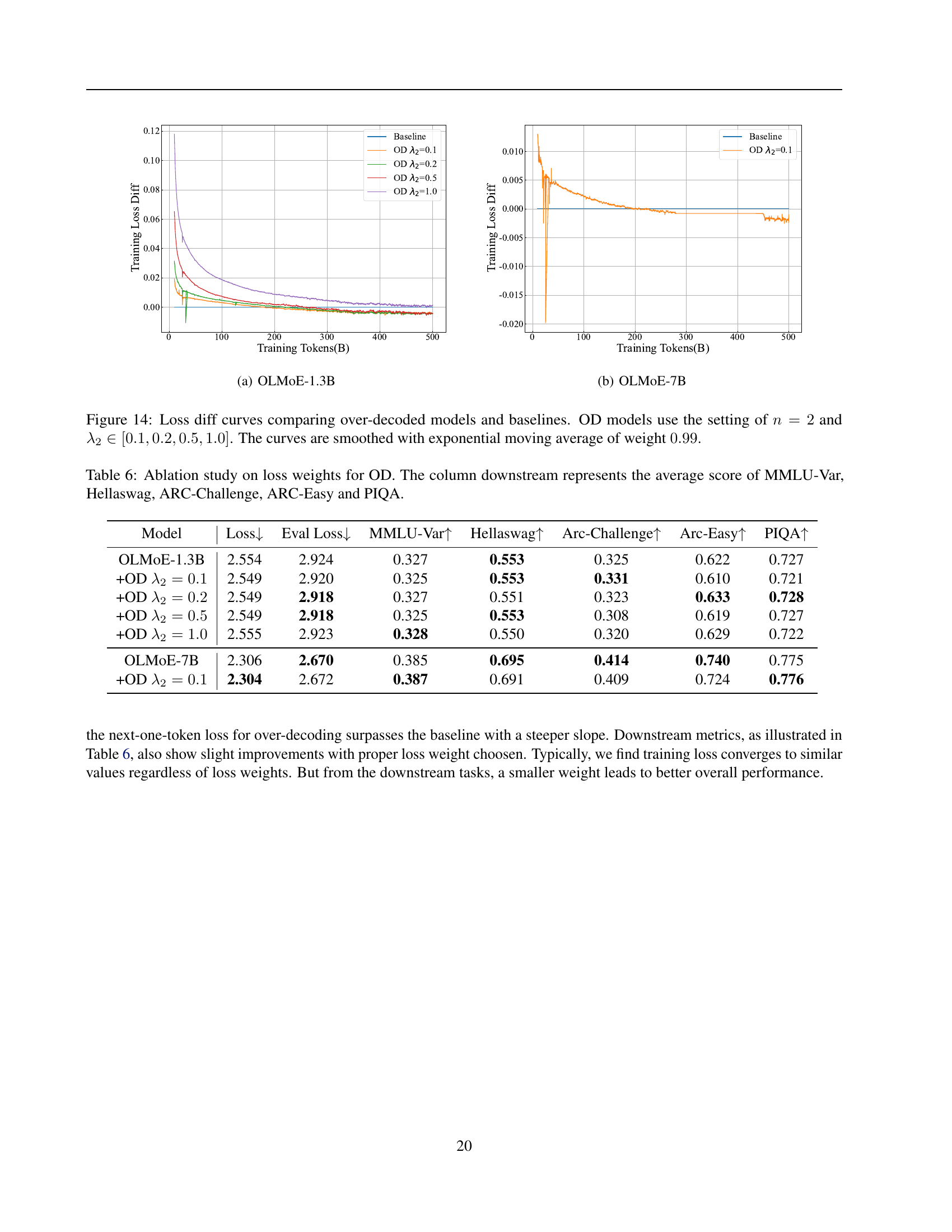
🔼 This table presents the results of an ablation study investigating the impact of different loss weight hyperparameters (λ2) on the performance of the Over-Decoding (OD) method. The study is conducted on two different sized models, OLMOE-1.3B and OLMOE-7B. The table shows the training loss, evaluation loss (Eval Loss), and average performance across multiple downstream tasks (MMLU-Var, Hellaswag, ARC-Challenge, ARC-Easy, and PIQA) for various values of λ2. This helps determine which weight setting produces the optimal balance between training loss and performance on downstream tasks.
read the caption
Table 6: Ablation study on loss weights for OD. The column downstream represents the average score of MMLU-Var, Hellaswag, ARC-Challenge, ARC-Easy and PIQA.

TL;DR#

Key Takeaways#

Why does it matter?#

Visual Insights#

In-depth insights#

Vocab Scaling Laws#

Over-Tokenization#

OE/OD Decoupling#

Engineering OE#

Future of Tokenization#

More visual insights#

Full paper#