TL;DR#
LLM post-training, crucial for enhancing language models, currently lacks sufficient open-source data for comprehensive analysis. This limits the ability to conduct large-scale comparative studies on the efficacy of various synthetic data generation methods and their impact on model performance. This paper introduces WILDCHAT-50M, a substantial dataset addressing this issue.
To address the data scarcity problem, the authors created WILDCHAT-50M, the largest public chat dataset to date, containing conversations from diverse models. They then built RE-WILD, an SFT (supervised fine-tuning) data mix, leveraging WILDCHAT-50M. RE-WILD outperforms state-of-the-art SFT mixtures, demonstrating the dataset’s value. The paper provides extensive analysis of model efficiency and response similarity, offering valuable insights for researchers working with LLMs and post-training techniques.
Key Takeaways#
Why does it matter?#
This paper is crucial for researchers in LLM post-training because it addresses the scarcity of large-scale, publicly available synthetic datasets for comparative analysis. WILDCHAT-50M, the dataset introduced, enables rigorous studies of synthetic data quality, offering valuable insights into effective data curation strategies and significantly advancing the field’s understanding of LLM post-training. This opens new avenues for research on data efficiency, model scaling, and developing more robust and reliable SFT methods.
Visual Insights#

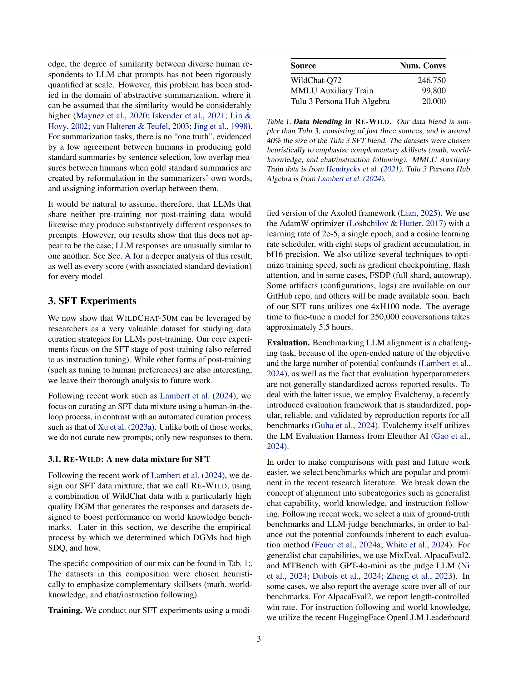
🔼 This figure presents a comparative analysis of the performance of different supervised fine-tuning (SFT) models on various benchmarks. The main finding is that RE-WILD, a novel data mix developed by the authors, outperforms existing strong baselines, particularly in generalist chat and instruction-following tasks. The chart visualizes these results across nine benchmarks, with MTBench scores scaled down for consistent representation. The data used to create the chart and the scores for each model can be found in the paper’s GitHub repository.
read the caption
Figure 1: Re-Wild outperforms strong baselines, on average, across nine benchmarks. In particular, it exhibits strong performance on generalist chat and instruction following benchmarks. MT Bench scores here are divided by 10, so that the scale is similar to our other evaluations. For the exact numeric scores for all models, please refer to our GitHub repository. Figure best viewed in color.
| Source | Num. Convs |
|---|---|
| WildChat-Q72 | 246,750 |
| MMLU Auxiliary Train | 99,800 |
| Tulu 3 Persona Hub Algebra | 20,000 |
🔼 The table details the composition of the RE-WILD dataset used for supervised fine-tuning (SFT). RE-WILD is a blend of three datasets: WildChat-Q72, MMLU Auxiliary Train, and Tulu 3 Persona Hub Algebra. It’s designed to be smaller and simpler than the Tulu 3 SFT mix, yet still provide a diverse range of skills, such as mathematical reasoning, world knowledge, and instruction following abilities. The sources of the data are cited. The table shows the number of conversations contributed by each dataset.
read the caption
Table 1: Data blending in Re-Wild. Our data blend is simpler than Tulu 3, consisting of just three sources, and is around 40% the size of the Tulu 3 SFT blend. The datasets were chosen heuristically to emphasize complementary skillsets (math, world-knowledge, and chat/instruction following). MMLU Auxiliary Train data is from Hendrycks et al. (2021), Tulu 3 Persona Hub Algebra is from Lambert et al. (2024).
In-depth insights#
Synthetic Data’s Role#
The research paper explores the crucial role of synthetic data in post-training large language models (LLMs). Synthetic data, generated by various models, acts as the primary training fuel, allowing for large-scale comparative analyses that would be otherwise infeasible with real-world data. The study highlights the importance of careful selection and curation of synthetic data, showing that data quality (SDQ) significantly impacts downstream LLM performance. Different data generating models (DGMs) produce data with varying qualities, and there’s no single dominant DGM. The paper introduces a novel data mix, showcasing the power of thoughtfully curated synthetic data to boost LLM performance, surpassing existing strong baselines. While model parameter count and response length aren’t reliable predictors of data quality, the study reveals that certain styling elements are inherited during supervised fine-tuning (SFT), suggesting that the choice of DGM significantly influences the overall quality and effectiveness of post-training.
WILDCHAT-50M Dataset#
The WILDCHAT-50M dataset represents a substantial contribution to the field of large language model (LLM) post-training. Its significance lies in its scale and diversity: encompassing chat transcripts generated by over 50 different open-weight LLMs, ranging from 0.5B to 104B parameters. This breadth allows for rigorous comparative analysis of various model architectures and their downstream effects on synthetic data quality. The dataset’s size (over 125 million chat transcripts) facilitates large-scale experiments, overcoming previous limitations in the availability of comparable publicly available data. WILDCHAT-50M’s potential impact extends beyond simple benchmarking: its use in creating the RE-WILD SFT mix, which outperforms existing methods with fewer samples, showcases its practical utility in advancing LLM post-training techniques. The availability of such a resource democratizes access to large-scale synthetic data for the research community, thereby fostering progress in LLM alignment and instruction tuning.
SFT Data Mix#
The concept of an ‘SFT Data Mix’ in the context of large language model (LLM) post-training involves carefully curating a dataset of diverse synthetic data to optimize the model’s performance on downstream tasks. This process recognizes that the quality of synthetic training data significantly impacts the effectiveness of supervised fine-tuning (SFT). A well-constructed SFT data mix aims to balance various data sources that may complement each other, covering different aspects of language proficiency like factual knowledge, reasoning skills, and adherence to instructions. The composition of the mix may be chosen heuristically, relying on insights about individual datasets’ strengths and potential for addressing specific weaknesses in the target LLM, or via a more sophisticated human-in-the-loop process. The selection of data sources is a critical factor, as models trained on this mix can exhibit varying degrees of success depending on the quality and characteristics of the underlying datasets, emphasizing the importance of strategic curation for optimal SFT results. The effectiveness of the SFT Data Mix is ultimately evaluated by measuring the fine-tuned model’s performance on various benchmarks. Therefore, creating a high-performing SFT data mix is a crucial yet challenging aspect of improving LLMs via post-training.
Model Efficiency#
Analyzing model efficiency in large language model (LLM) post-training is crucial for practical applications. The computational cost of training and inference significantly impacts the scalability and accessibility of these techniques. Throughput efficiency, measured by tokens processed per second, reveals trade-offs between model size and speed. Larger models, while potentially more powerful, often exhibit lower throughput. VRAM efficiency is another critical aspect, as models exceeding available memory require techniques like gradient checkpointing, impacting runtime and performance. The authors highlight the importance of understanding these trade-offs to inform data curation strategies and to enable efficient scaling of LLM post-training, especially for researchers with limited computational resources. Data generation cost is also a factor, as generating large datasets can be expensive, particularly when using a diverse range of models. Thus, balancing model size, throughput, VRAM efficiency, and data generation costs is essential for optimization.
Future Work#
Future research directions stemming from this paper on synthetic data in LLM post-training could explore several avenues. Expanding the dataset is crucial; WILDCHAT-50M’s size is impressive, but incorporating even more models and data points would strengthen analyses. A focus on diverse data generation methods beyond the current selection, including investigation into the impact of different prompt engineering techniques, would refine our understanding of SDQ. Investigating other post-training methods beyond SFT, such as reinforcement learning techniques, would reveal if the observed trends in data quality hold across different training paradigms. Furthermore, a deeper dive into the relationship between DGM characteristics and downstream LLM performance could unveil predictive factors for improved synthetic data selection. Finally, research into new evaluation metrics for LLM outputs is vital, especially to better capture more nuanced aspects of quality than current benchmarks allow. Addressing these points will allow for a more comprehensive understanding of how to effectively leverage synthetic data in improving LLMs.
More visual insights#
More on figures

🔼 This figure shows the impact of increasing the size of the training dataset on the performance of Supervised Fine-Tuning (SFT). The x-axis represents the size of the training dataset, while the y-axis shows the average performance across various benchmarks (MixEval, AlpacaEval2-LC, MTBench/10, and OpenLLM LB2). Different colored bars represent different Data Generating Models (DGMs). The results indicate that larger datasets generally lead to improved SFT performance; however, the degree of improvement varies depending on the quality of the synthetic data generated by the DGM. For models like GPT-3.5, performance plateaus relatively quickly with increased data size, while other DGMs show consistent improvement with larger datasets. This highlights that data quality and the model used for data generation significantly influence the effectiveness of data scaling in SFT.
read the caption
Figure 2: Data scaling improves SFT performance. The effect is, however, somewhat dependent on SDQ – for DGMs such as GPT 3.5, the benefits taper off relatively quickly, but for the other three DGMs we consider, they continue to increase. Avg is the average performance over (MixEval, AlpacaEval2-LC, MTBench / 10, OpenLLM LB 2).

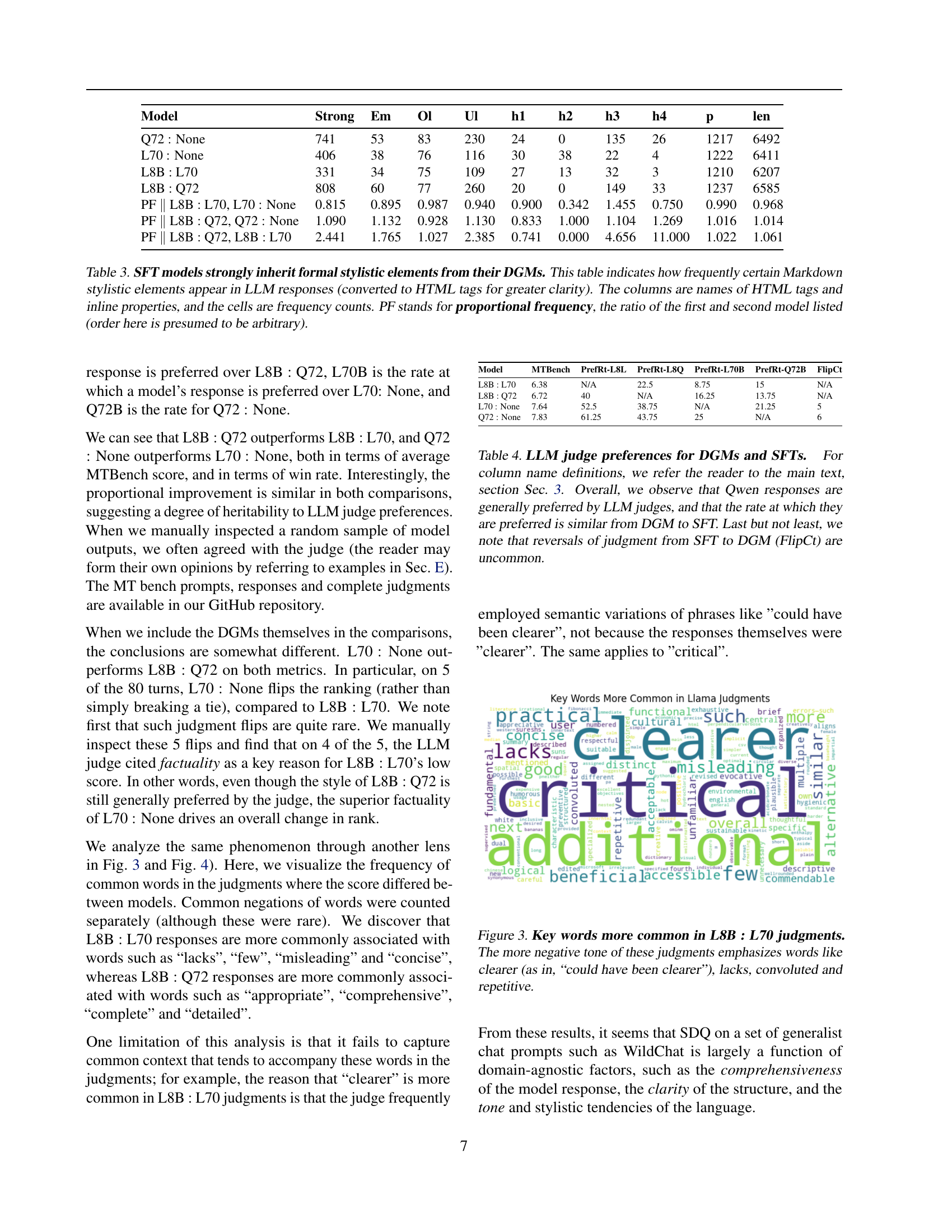
🔼 Figure 3 is a word cloud showing the words that appeared most frequently in the human evaluator’s feedback when comparing the performance of two fine-tuned language models (LLMs): L8B:L70 (Llama-3.1 8B Base fine-tuned on Llama-3.3-70B responses) and L8B:Q72 (Llama-3.1 8B Base fine-tuned on Qwen-2.5-72B responses). The word cloud visualizes the negative sentiment expressed in the evaluations of L8B:L70. The prominent words, such as ’lacks,’ ‘convoluted,’ and ‘repetitive,’ highlight the perceived shortcomings of L8B:L70 in comparison to L8B:Q72. The presence of ‘clearer’ indicates that the judges desired more clarity in L8B:L70’s outputs. The word cloud provides a concise visual summary of the qualitative aspects of model performance.
read the caption
Figure 3: Key words more common in L8B : L70 judgments. The more negative tone of these judgments emphasizes words like clearer (as in, “could have been clearer”), lacks, convoluted and repetitive.

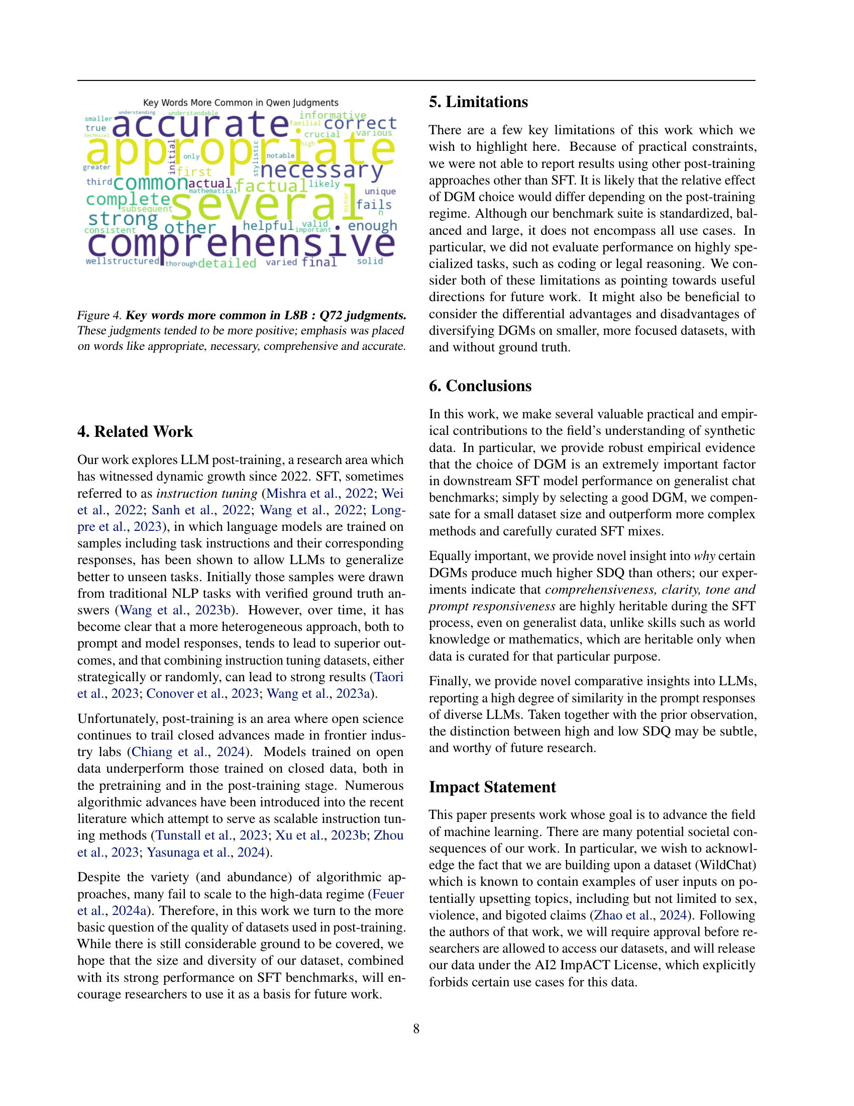
🔼 Figure 4 is a word cloud visualizing the words that frequently appeared in the LLM judge’s feedback when comparing the performance of Llama-3.1-8B-Base fine-tuned on Qwen-2.5-72B responses against other models. The word cloud shows that the judges’ comments were generally more positive for this model. Words like ‘appropriate,’ ’necessary,’ ‘comprehensive,’ and ‘accurate’ were prominently featured, indicating that the model’s responses were perceived as well-suited to the task and of high quality.
read the caption
Figure 4: Key words more common in L8B : Q72 judgments. These judgments tended to be more positive; emphasis was placed on words like appropriate, necessary, comprehensive and accurate.
More on tables
| Model | MTBench | AlpacaEval | BBH | GPQA | MATH | MUSR | IFEval | MMLU Pro | MixEval |
|---|---|---|---|---|---|---|---|---|---|
| Q72 | 6.86 | 41.00 | 48.07 | 29.32 | 5.62 | 40.27 | 36.78 | 30.38 | 64.50 |
| L8I | 6.26 | 21.12 | 45.83 | 30.35 | 4.49 | 37.32 | 38.26 | 32.54 | 65.30 |
| L70 | 6.23 | 24.91 | 46.57 | 29.97 | 4.08 | 39.44 | 33.83 | 30.85 | 64.60 |
| Q7 | 6.03 | 17.26 | 48.72 | 29.90 | 2.93 | 42.11 | 29.39 | 30.34 | 61.30 |
| CRP | 6.05 | 13.44 | 49.27 | 30.82 | 4.16 | 38.79 | 28.47 | 31.64 | 60.30 |
| JMB | 6.05 | 25.14 | 47.36 | 28.28 | 3.93 | 37.50 | 25.69 | 29.32 | 57.40 |
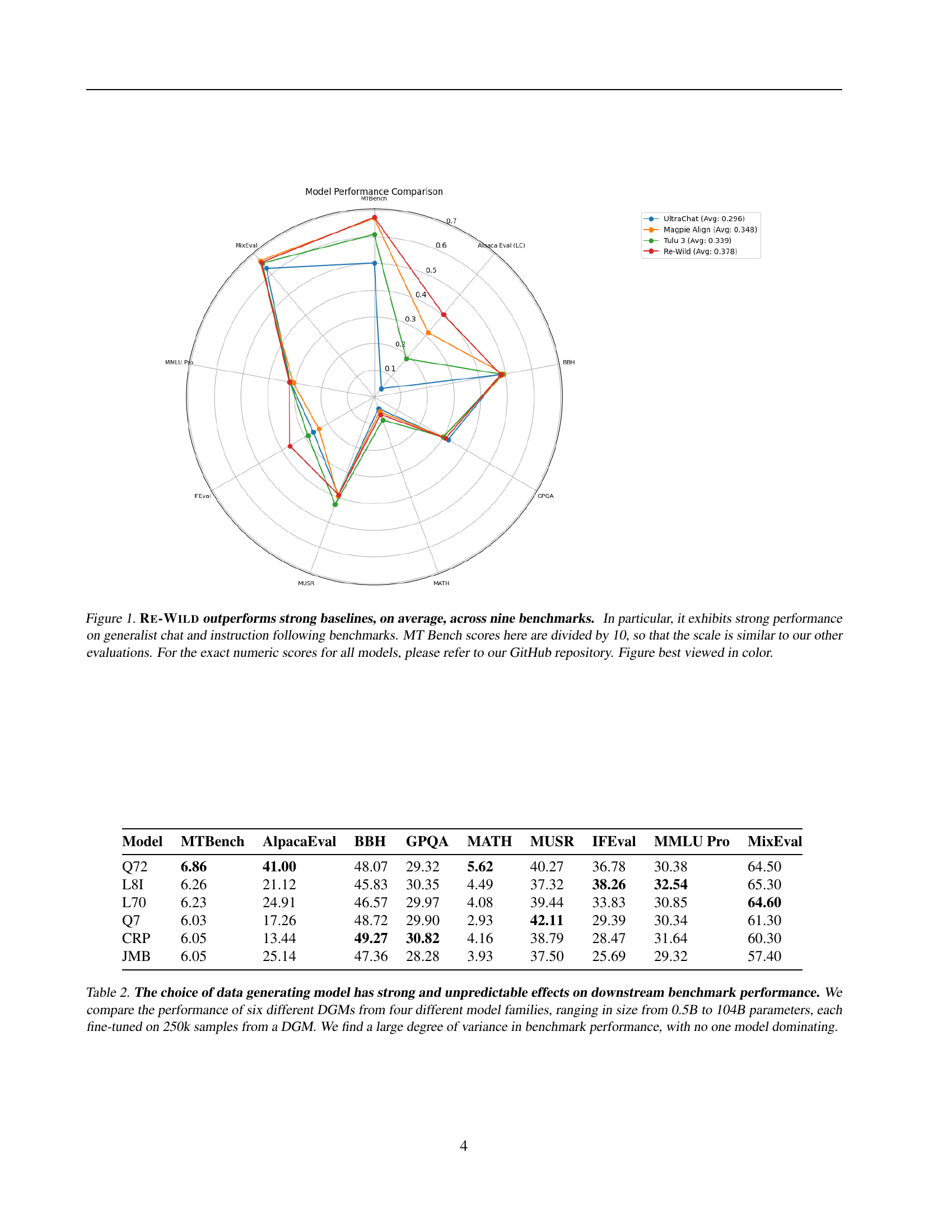
🔼 This table presents a comparative analysis of six different large language models (LLMs) used as data generators for supervised fine-tuning (SFT). Each LLM, ranging in size from 0.5 billion to 104 billion parameters, generated 250,000 chat transcripts. The performance of the fine-tuned models is then evaluated across various benchmarks, revealing that the choice of data-generating model has a significant and unpredictable impact on the final performance. There is a considerable amount of variance in the results, with no single model consistently outperforming the others.
read the caption
Table 2: The choice of data generating model has strong and unpredictable effects on downstream benchmark performance. We compare the performance of six different DGMs from four different model families, ranging in size from 0.5B to 104B parameters, each fine-tuned on 250k samples from a DGM. We find a large degree of variance in benchmark performance, with no one model dominating.
| Model | Strong | Em | Ol | Ul | h1 | h2 | h3 | h4 | p | len |
|---|---|---|---|---|---|---|---|---|---|---|
| Q72 : None | 741 | 53 | 83 | 230 | 24 | 0 | 135 | 26 | 1217 | 6492 |
| L70 : None | 406 | 38 | 76 | 116 | 30 | 38 | 22 | 4 | 1222 | 6411 |
| L8B : L70 | 331 | 34 | 75 | 109 | 27 | 13 | 32 | 3 | 1210 | 6207 |
| L8B : Q72 | 808 | 60 | 77 | 260 | 20 | 0 | 149 | 33 | 1237 | 6585 |
| PF L8B : L70, L70 : None | 0.815 | 0.895 | 0.987 | 0.940 | 0.900 | 0.342 | 1.455 | 0.750 | 0.990 | 0.968 |
| PF L8B : Q72, Q72 : None | 1.090 | 1.132 | 0.928 | 1.130 | 0.833 | 1.000 | 1.104 | 1.269 | 1.016 | 1.014 |
| PF L8B : Q72, L8B : L70 | 2.441 | 1.765 | 1.027 | 2.385 | 0.741 | 0.000 | 4.656 | 11.000 | 1.022 | 1.061 |
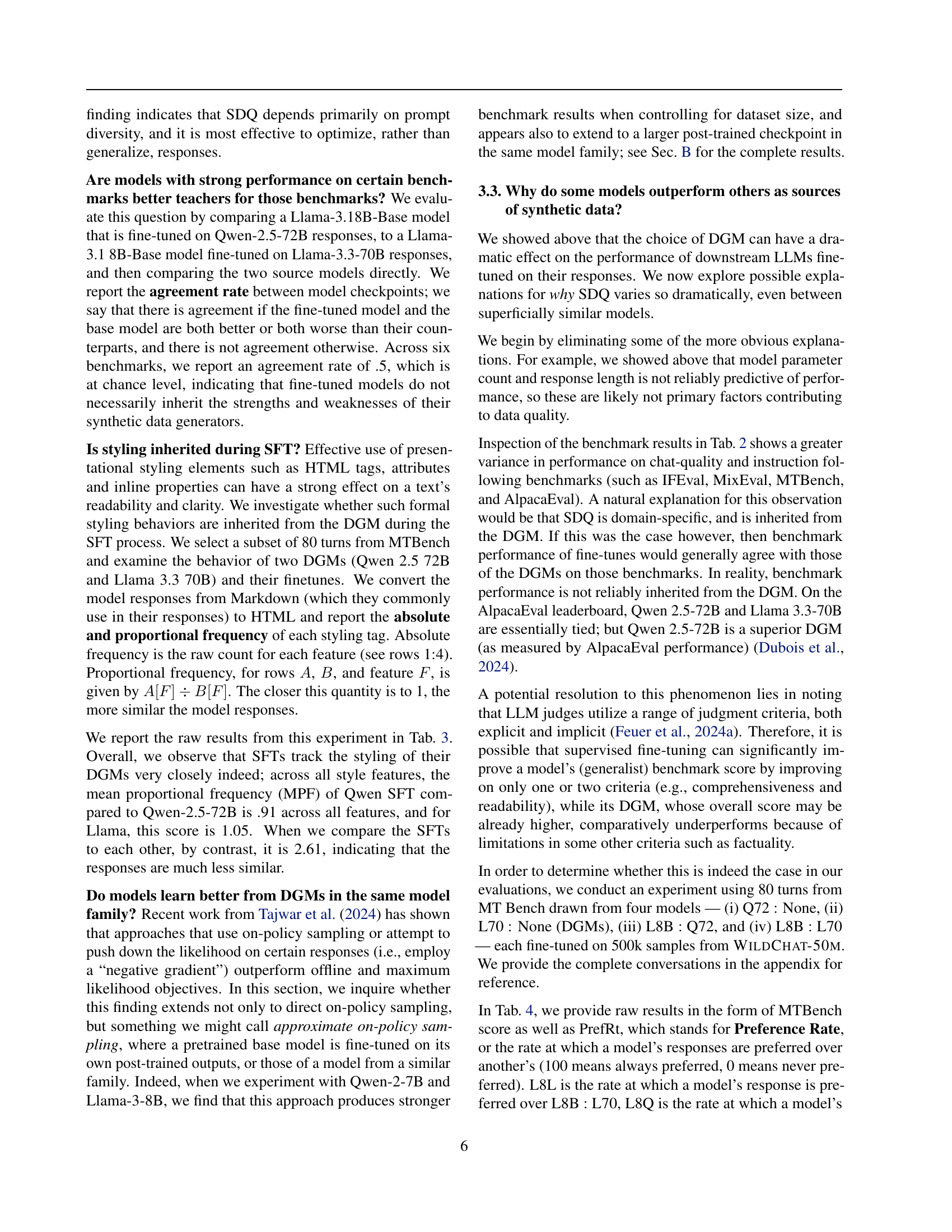
🔼 Table 3 presents a detailed analysis of stylistic element inheritance during supervised fine-tuning (SFT) of large language models (LLMs). It compares the frequency of specific Markdown formatting elements (converted to HTML for clarity) in the outputs of both original data-generating models (DGMs) and their corresponding SFT models. The table shows the absolute frequency counts of various HTML tags and inline properties in 80 turns from the MTBench dataset, as well as the proportional frequency of these elements between the DGM and its SFT counterpart. The ‘proportional frequency’ metric helps assess how closely the SFT model’s style matches that of the DGM it was trained on, enabling researchers to understand the extent of style transfer during SFT and its potential impact on downstream model performance. Note that the order of the models in computing the proportional frequency is arbitrary.
read the caption
Table 3: SFT models strongly inherit formal stylistic elements from their DGMs. This table indicates how frequently certain Markdown stylistic elements appear in LLM responses (converted to HTML tags for greater clarity). The columns are names of HTML tags and inline properties, and the cells are frequency counts. PF stands for proportional frequency, the ratio of the first and second model listed (order here is presumed to be arbitrary).
| Model | MTBench | PrefRt-L8L | PrefRt-L8Q | PrefRt-L70B | PrefRt-Q72B | FlipCt |
|---|---|---|---|---|---|---|
| L8B : L70 | 6.38 | N/A | 22.5 | 8.75 | 15 | N/A |
| L8B : Q72 | 6.72 | 40 | N/A | 16.25 | 13.75 | N/A |
| L70 : None | 7.64 | 52.5 | 38.75 | N/A | 21.25 | 5 |
| Q72 : None | 7.83 | 61.25 | 43.75 | 25 | N/A | 6 |
🔼 This table presents the results of a comparative analysis on the performance of different Data Generating Models (DGMs) and their corresponding Supervised Fine-Tuning (SFT) models. It evaluates how often LLMs prefer the responses generated by each DGM and SFT model, using various benchmarks. The ‘Preference Rate’ columns show the percentage of times one model’s response was preferred over another across different evaluation metrics (Benchmarks). The ‘FlipCt’ column represents the number of instances where the ranking between the DGM and SFT model is reversed in terms of preference. The analysis highlights the strong preference for Qwen responses among LLMs and the consistent preference pattern observed between DGMs and SFT models, demonstrating the impact of the original DGM’s choice on the SFT model performance.
read the caption
Table 4: LLM judge preferences for DGMs and SFTs. For column name definitions, we refer the reader to the main text, section Sec. 3. Overall, we observe that Qwen responses are generally preferred by LLM judges, and that the rate at which they are preferred is similar from DGM to SFT. Last but not least, we note that reversals of judgment from SFT to DGM (FlipCt) are uncommon.
| Model | avg_rouge1 | std_rouge1 | avg_rougeL | std_rougeL | avg_meteor | std_meteor |
|---|---|---|---|---|---|---|
| Mixtral-8x7B-Instruct | 0.37 | 0.11 | 0.19 | 0.06 | 0.20 | 0.05 |
| Llama-3.1-Nemotron-70B-Instruct | 0.37 | 0.06 | 0.23 | 0.05 | 0.20 | 0.05 |
| Qwen2.5-72B-Instruct | 0.34 | 0.09 | 0.17 | 0.05 | 0.17 | 0.05 |
| Mistral-7B-wizardlm | 0.34 | 0.07 | 0.22 | 0.06 | 0.16 | 0.05 |
| Mistral-7B-sharegpt-vicuna | 0.34 | 0.06 | 0.18 | 0.03 | 0.18 | 0.04 |
| Mistral-7B-Base-SFT-IPO | 0.33 | 0.11 | 0.17 | 0.05 | 0.19 | 0.06 |
| internlm2_5-20b-chat | 0.33 | 0.08 | 0.15 | 0.03 | 0.20 | 0.06 |
| Llama-3.1-70B-Instruct | 0.33 | 0.10 | 0.16 | 0.05 | 0.16 | 0.06 |
| Llama-3.3-70B-Instruct | 0.33 | 0.09 | 0.17 | 0.04 | 0.20 | 0.05 |
| Llama-2-7b-chat-hf | 0.32 | 0.09 | 0.19 | 0.07 | 0.20 | 0.06 |
| Mistral-7B-Base-SFT-CPO | 0.32 | 0.07 | 0.17 | 0.04 | 0.18 | 0.05 |
| Qwen2-7B-Instruct | 0.32 | 0.08 | 0.15 | 0.04 | 0.17 | 0.06 |
| Llama-3-8B-ShareGPT-112K | 0.31 | 0.09 | 0.18 | 0.07 | 0.15 | 0.06 |
| Qwen2.5-Coder-32B-Instruct | 0.31 | 0.10 | 0.15 | 0.05 | 0.18 | 0.05 |
| Llama-3-8B-Magpie-Pro-SFT-200K | 0.30 | 0.15 | 0.18 | 0.09 | 0.17 | 0.09 |
| google_gemma-2-9b-it | 0.30 | 0.10 | 0.16 | 0.06 | 0.14 | 0.06 |
| AI21-Jamba-1.5-Mini | 0.29 | 0.13 | 0.17 | 0.08 | 0.14 | 0.06 |
| OpenHermes-2-Mistral-7B | 0.28 | 0.09 | 0.16 | 0.06 | 0.15 | 0.07 |
| Llama-3-Base-8B-SFT-ORPO | 0.27 | 0.07 | 0.14 | 0.03 | 0.22 | 0.05 |
| google_gemma-2-27b-it | 0.27 | 0.04 | 0.13 | 0.02 | 0.15 | 0.03 |
| OpenHermes-2.5-Mistral-7B | 0.27 | 0.06 | 0.15 | 0.04 | 0.13 | 0.04 |
| Mistral-7B-Base-SFT-SLiC-HF | 0.26 | 0.13 | 0.14 | 0.07 | 0.13 | 0.07 |
| Mistral-7B-Base-SFT-KTO | 0.25 | 0.05 | 0.13 | 0.04 | 0.11 | 0.04 |
| Ministral-8B-Instruct-2410 | 0.24 | 0.13 | 0.12 | 0.07 | 0.13 | 0.09 |
| Llama-3-Base-8B-SFT-RDPO | 0.23 | 0.06 | 0.13 | 0.03 | 0.19 | 0.03 |
| Mistral-7B-Base-SFT-RRHF | 0.19 | 0.06 | 0.08 | 0.02 | 0.16 | 0.04 |
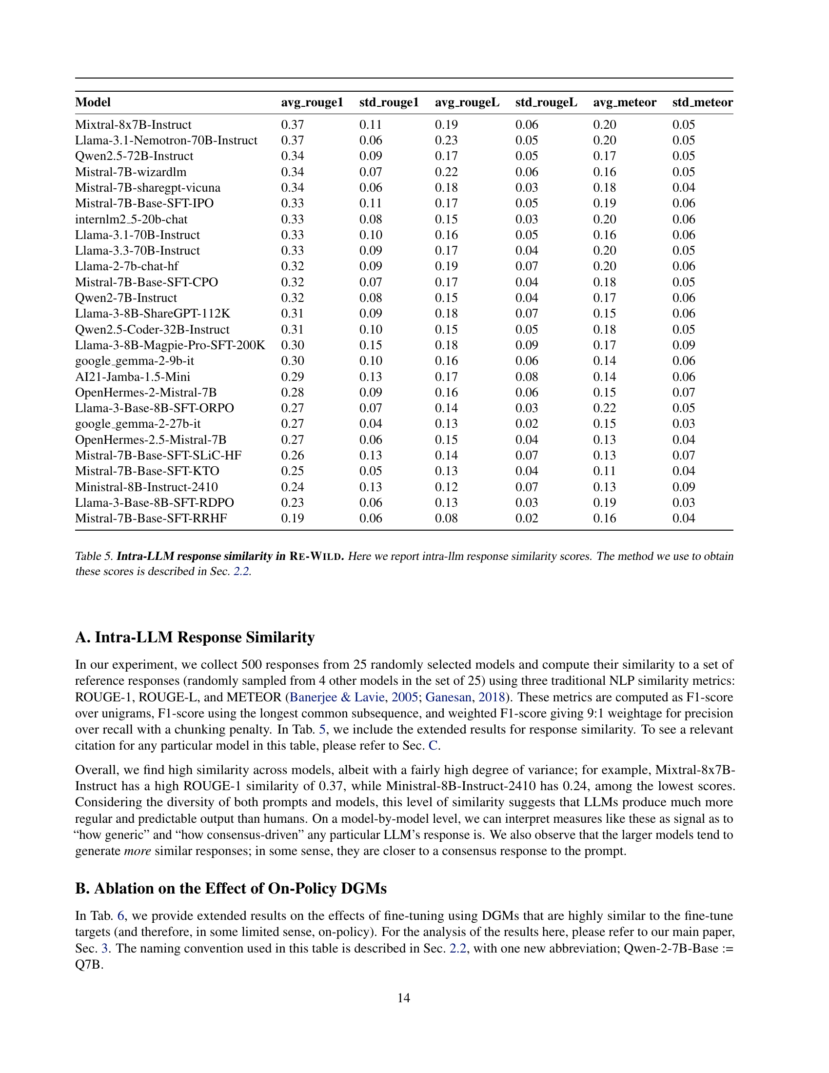
🔼 This table presents the results of an intra-LLM response similarity analysis conducted on the WILDCHAT-50M dataset. It shows how similar the responses generated by different large language models (LLMs) are to each other, using three common Natural Language Processing (NLP) metrics: ROUGE-1, ROUGE-L, and METEOR. The metrics measure the overlap between the responses. Higher scores indicate greater similarity. The table shows that the models exhibit a relatively high degree of response similarity. The methodology used to calculate these scores is described in detail in Section 2.2 of the paper. This similarity across models is noteworthy, given the diversity of prompts and the range of models used in the study. It suggests that LLMs, regardless of their size or training, tend to generate responses that are more similar to each other than one might expect based on human responses to the same prompts. This observation hints at the relatively limited diversity found in LLMs’ responses.
read the caption
Table 5: Intra-LLM response similarity in Re-Wild. Here we report intra-llm response similarity scores. The method we use to obtain these scores is described in Sec. 2.2.
| Model | MTBench | AlpacaEval | BBH | GPQA | MATH | MUSR | IFEval | MMLU Pro | MixEval | Avg |
|---|---|---|---|---|---|---|---|---|---|---|
| L8B : L8I | 6.26 | 21.12 | 0.46 | 0.30 | 0.04 | 0.37 | 0.38 | 0.33 | 0.65 | 0.36 |
| L8B : Q7 | 6.03 | 17.26 | 0.49 | 0.30 | 0.03 | 0.42 | 0.29 | 0.30 | 0.61 | 0.35 |
| L8B : L70 | 6.23 | 24.91 | 0.47 | 0.30 | 0.04 | 0.39 | 0.34 | 0.31 | 0.65 | 0.36 |
| Q7B : L8I | 6.51 | 15.87 | 0.51 | 0.29 | 0.17 | 0.43 | 0.35 | 0.39 | 0.61 | 0.39 |
| Q7B : Q7 | 6.69 | 27.09 | 0.54 | 0.31 | 0.19 | 0.45 | 0.40 | 0.42 | 0.69 | 0.43 |
| Q7B : Q72 | 7.25 | 36.68 | 0.54 | 0.32 | 0.21 | 0.43 | 0.34 | 0.43 | 0.65 | 0.42 |
| Q7 : None | 7.17 | 33.14 | 0.55 | 0.33 | 0.19 | 0.45 | 0.42 | 0.40 | 0.73 | 0.44 |
| L8I : None | 7.20 | 30.84 | 0.51 | 0.33 | 0.12 | 0.40 | 0.42 | 0.38 | 0.74 | 0.41 |
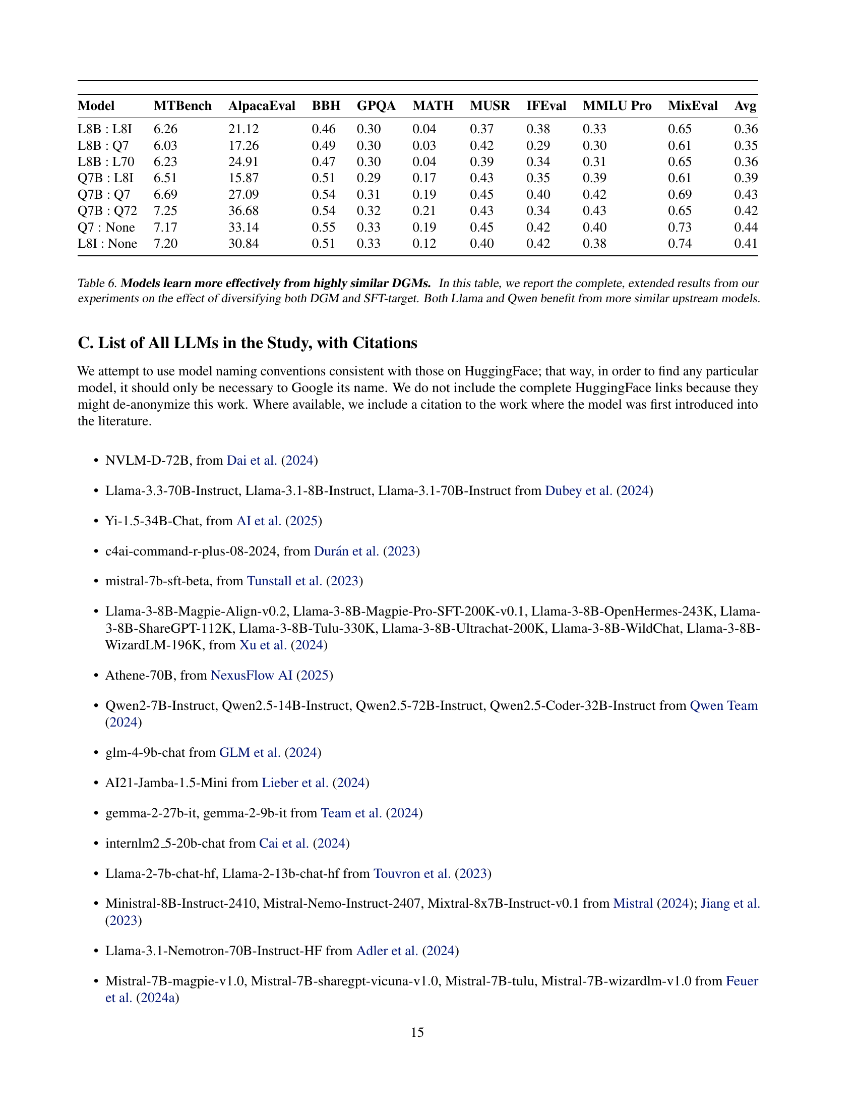
🔼 Table 6 presents a comprehensive analysis of the impact of using similar data generating models (DGMs) during supervised fine-tuning (SFT) on the performance of large language models (LLMs). It compares different combinations of base LLMs (Llama and Qwen) and fine-tuned models, each trained on datasets generated by various DGMs. The table shows that fine-tuning an LLM on data from a similar DGM leads to significantly better performance across various benchmarks compared to using data from dissimilar DGMs. This highlights the importance of DGM selection for effective SFT and indicates that models might learn more effectively when the training data reflects their own characteristics and style.
read the caption
Table 6: Models learn more effectively from highly similar DGMs. In this table, we report the complete, extended results from our experiments on the effect of diversifying both DGM and SFT-target. Both Llama and Qwen benefit from more similar upstream models.
| Model | MTBench | Alpaca Eval (LC) | BBH | GPQA | MATH | MUSR | IFEval | MMLU Pro | MixEval | Avg |
|---|---|---|---|---|---|---|---|---|---|---|
| L8B : Q7 (500k) | 6.33 | 19.51 | 0.48 | 0.28 | 0.04 | 0.40 | 0.33 | 0.30 | 0.64 | 0.35 |
| L8B : L8I (500k) | 6.52 | 21.03 | 0.46 | 0.32 | 0.05 | 0.39 | 0.42 | 0.32 | 0.66 | 0.37 |
| L8B : L8I + Q7 (500k) | 6.43 | 18.57 | 0.47 | 0.28 | 0.05 | 0.41 | 0.34 | 0.32 | 0.64 | 0.36 |
| L8B : Q72 (500k) | 6.51 | 41.67 | 0.48 | 0.29 | 0.05 | 0.39 | 0.39 | 0.30 | 0.66 | 0.37 |
| L8B : L70 (500k) | 6.39 | 27.38 | 0.46 | 0.31 | 0.04 | 0.36 | 0.38 | 0.32 | 0.65 | 0.36 |
| L8B : Q72 + L70 (500k) | 6.82 | 39.93 | 0.48 | 0.29 | 0.04 | 0.38 | 0.38 | 0.31 | 0.65 | 0.36 |
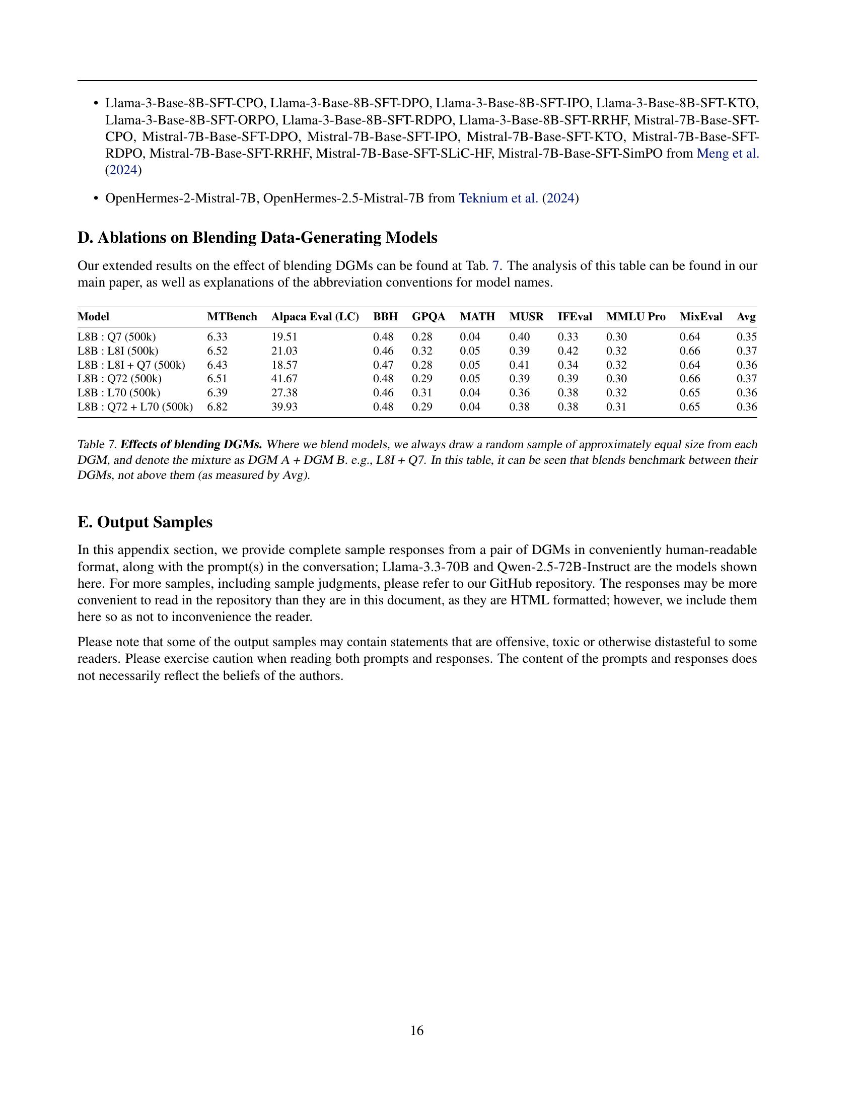
🔼 This table presents the results of experiments assessing the impact of blending different Data Generating Models (DGMs) on the performance of downstream models. The experiments involved fine-tuning models on datasets created by mixing data from different DGMs in roughly equal proportions. The table shows the performance of these models on various benchmark tasks (MTBench, AlpacaEval, BBH, GPQA, MATH, MUSR, IFEval, MMLU, Pro, and MixEval). The ‘Avg’ column shows the average performance across all benchmarks. The results indicate that blending DGMs generally leads to performance that falls between the performance of the individual DGMs used in the mixture, rather than surpassing the performance of the best individual DGM.
read the caption
Table 7: Effects of blending DGMs. Where we blend models, we always draw a random sample of approximately equal size from each DGM, and denote the mixture as DGM A + DGM B. e.g., L8I + Q7. In this table, it can be seen that blends benchmark between their DGMs, not above them (as measured by Avg).
Full paper#