TL;DR#
Training large language models (LLMs) is computationally expensive, requiring high-bandwidth communication across many accelerators. Existing distributed training methods like DiLoCo alleviate co-location constraints but still suffer from high peak bandwidth needs. This creates a significant hurdle to scaling LLM training further.
This paper introduces Streaming DiLoCo, which significantly reduces peak bandwidth needs by synchronizing only subsets of parameters in sequence, rather than all at once. It also overlaps worker computation with communication, which minimizes downtime and speeds up the process. Lastly, the data exchanged between workers is quantized to further reduce the bandwidth needed. Through these three contributions, Streaming DiLoCo enables efficient training of billion-scale parameter LLMs with substantially reduced bandwidth requirements.
Key Takeaways#
Why does it matter?#
This paper is crucial for researchers in distributed machine learning, particularly those working with large language models. It offers practical solutions to overcome major bandwidth limitations, which is a critical bottleneck in training massive models. The techniques presented, such as overlapping communication and parameter subset synchronization, are widely applicable and pave the way for more efficient and scalable training paradigms. The findings are significant because they demonstrate substantial bandwidth reduction while maintaining model performance. This opens doors for training even larger and more complex models in the future, advancing the capabilities of AI systems.
Visual Insights#

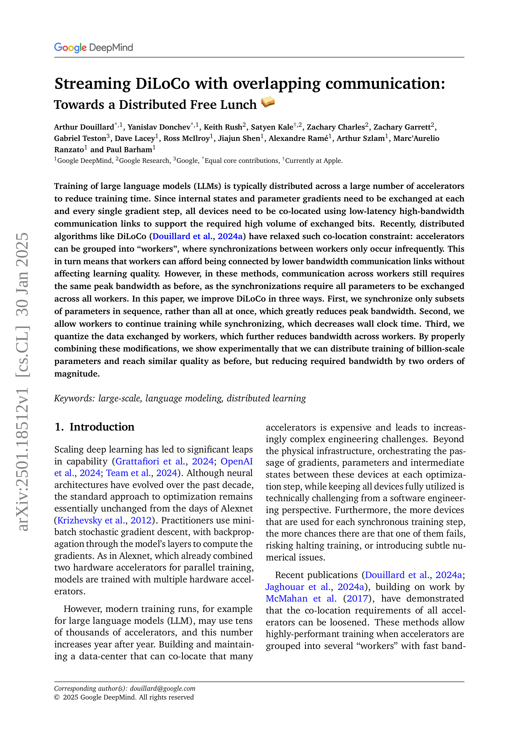
🔼 The figure illustrates the Streaming DiLoCo algorithm. It depicts four replicas (M=4), each independently processing their data for a specified number of inner optimization steps. After these steps, instead of synchronizing the entire model parameters, they only synchronize a single fragment (p={1,2,3}) of the parameters. This process repeats iteratively. Each fragment is a subset of layers in the transformer model. Importantly, the diagram only visualizes the streaming partial updates (section 2.2), excluding the quantized communication and overlapping techniques (sections 2.3 and 2.4).
read the caption
Figure 1: Streaming DiLoCo: each replica trains independently for dozen of inner optimization steps, and then synchronize a single fragment during outer optimization. In this figure, there are M=4𝑀4M=4italic_M = 4 replicas with p={1,2,3}𝑝123p=\{1,2,3\}italic_p = { 1 , 2 , 3 } fragments. Each fragment can be made of several transformer layers. Note that this figure only showcases the streaming partial updates (subsection 2.2) and not the quantized communication overlapping (subsection 2.3 and 2.4).
| Method | Token Budget | Hours spent w/ Gbits/s | Hours spent w/ 1 Gbits/s | Terabytes exchanged | Eval Loss | HellaSwag | Piqa | Arc Easy |
|---|---|---|---|---|---|---|---|---|
| Data-Parallel | 25B | 0.67 | 109 | 441 | 2.67 | 42.09 | 67.35 | 40.42 |
| 100B | 2.7 | 438 | 1,767 | 2.52 | 49.78 | 69.15 | 44.03 | |
| 250B | 6.75 | 1097 | 4,418 | 2.45 | 53.86 | 70.45 | 44.21 | |
| Streaming DiLoCo with overlapped FP4 communication | 25B | 0.67 | 0.88 | 1.10 | 2.66 | 42.08 | 67.46 | 38.42 |
| 100B | 2.7 | 3.5 | 4.42 | 2.51 | 49.98 | 69.96 | 44.03 | |
| 250B | 6.75 | 8.75 | 11.05 | 2.45 | 54.24 | 71.38 | 41.92 |
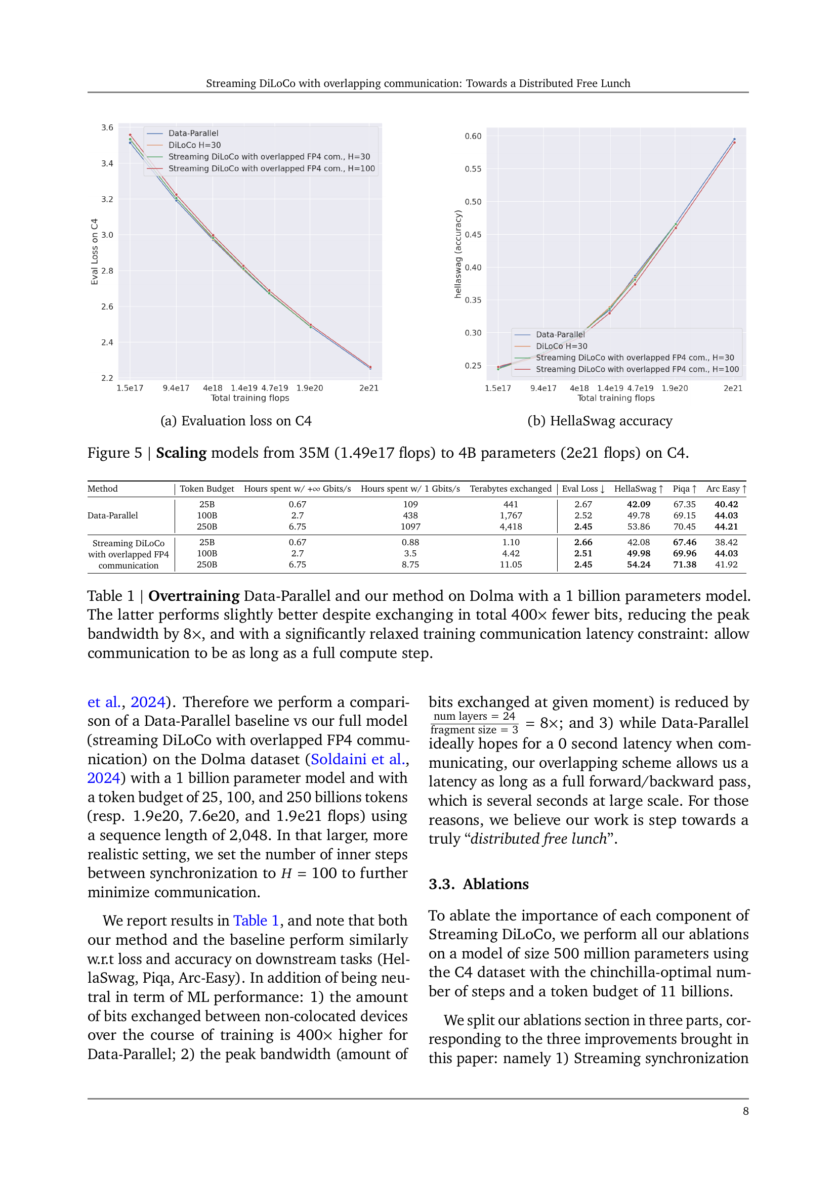
🔼 This table compares the performance of Data-Parallel and Streaming DiLoCo on the Dolma dataset when training a 1 billion parameter model. It highlights Streaming DiLoCo’s superior performance despite using significantly less communication bandwidth (400 times fewer bits and 8 times lower peak bandwidth). A key advantage of Streaming DiLoCo is its relaxed communication latency constraint; it allows for communication delays equal to a full compute step.
read the caption
Table 1: Overtraining Data-Parallel and our method on Dolma with a 1 billion parameters model. The latter performs slightly better despite exchanging in total 400×400\times400 × fewer bits, reducing the peak bandwidth by 8×8\times8 ×, and with a significantly relaxed training communication latency constraint: allow communication to be as long as a full compute step.
In-depth insights#
DiLoCo’s Streaming#
DiLoCo’s Streaming introduces a novel approach to distributed training of large language models (LLMs) by synchronizing only subsets of parameters sequentially, rather than all at once. This significantly reduces peak bandwidth requirements, a major bottleneck in large-scale LLM training. Overlapping communication with computation further enhances efficiency by allowing concurrent training and synchronization, minimizing idle time. The method also employs low-precision quantization of exchanged gradients to further reduce bandwidth demands. These combined optimizations enable training of billion-scale parameter models with significantly reduced bandwidth—two orders of magnitude lower—while maintaining comparable learning quality. The technique is shown to be robust, performing well across various model scales and hyperparameter settings, and even with heterogeneous worker environments. The results suggest that this approach, which efficiently manages communication overhead, represents a significant step towards a distributed free lunch scenario—achieving high performance at minimal communication costs.
Overlapping Comm.#
The concept of “Overlapping Comm.” in a distributed deep learning context likely refers to techniques that overlap communication and computation to improve training efficiency. Traditional approaches often stall computation while waiting for data transfers between nodes, leading to idle time. Overlapping communication cleverly schedules communication tasks concurrently with computation, effectively minimizing idle time and reducing overall training time. Careful scheduling and efficient communication protocols are crucial for successful implementation; otherwise, overlapping might lead to performance degradation due to contention or resource conflicts. This approach is particularly beneficial for large-scale models where communication overheads become significant, offering a path towards a “distributed free lunch” by achieving similar results with substantially lower communication costs. The success of overlapping relies on minimizing communication latency and maximizing computational throughput, and might involve techniques like pipelining, asynchronous operations, or specialized hardware.
Quantization Effects#
The heading ‘Quantization Effects’ in a research paper likely explores how reducing the precision of numerical representations (e.g., from 32-bit floating-point to 4-bit) impacts the overall model performance and training process. A key focus would be the trade-off between reduced computational cost (memory and bandwidth) and potential loss in accuracy. The analysis might involve experiments comparing models trained with different quantization levels, examining metrics like model accuracy, training speed, and convergence behavior. The results section would likely discuss whether the benefits of reduced resource usage outweigh the costs of decreased accuracy. A detailed breakdown of the impact on various model components (e.g., weights, activations, gradients) is crucial. The paper may also investigate different quantization techniques and their relative effectiveness, as well as methods for mitigating the negative impacts of quantization. The findings could offer valuable insights for optimizing large-scale models where memory and computational constraints are significant. Ultimately, the goal is to determine the optimal quantization level that balances accuracy and efficiency for a specific application.
LLM Scaling Tests#
LLM scaling tests in research papers typically involve evaluating model performance across various sizes, focusing on how key metrics change with increased scale. This includes analyzing computational cost, memory usage, and training time as model parameters grow. A crucial aspect is assessing whether improvements in performance scale linearly or sublinearly with increased resources. The tests should carefully consider the impact of different hardware architectures and training strategies, reporting results on benchmark datasets for various tasks. Careful consideration of data parallelism strategies is vital in analyzing scaling behavior, as well as the exploration of techniques to mitigate the communication bottleneck frequently encountered in large-scale training. Ultimately, LLM scaling tests aim to determine the optimal balance between model size and performance, providing valuable insights into the efficiency and cost-effectiveness of different training approaches and informing future LLM development.
Future Work#
The authors propose several avenues for future research. Scaling the number of DiLoCo replicas efficiently is crucial, especially considering the impact on token budget and overall training efficiency. They also highlight the potential of co-designing architectures and training paradigms, leveraging the reduced communication overhead to explore new parallelisms. This could include techniques like modular constellations of smaller models that leverage compute arbitrage across heterogeneous devices globally. The study of how to effectively tune and scale new distributed methods for large language models, especially under realistic constraints like variable device speeds and heterogeneous infrastructure, is also highlighted as a key area to further investigate. Finally, the impact of these techniques in training different types of models (other than LLMs) warrants exploration.
More visual insights#
More on figures

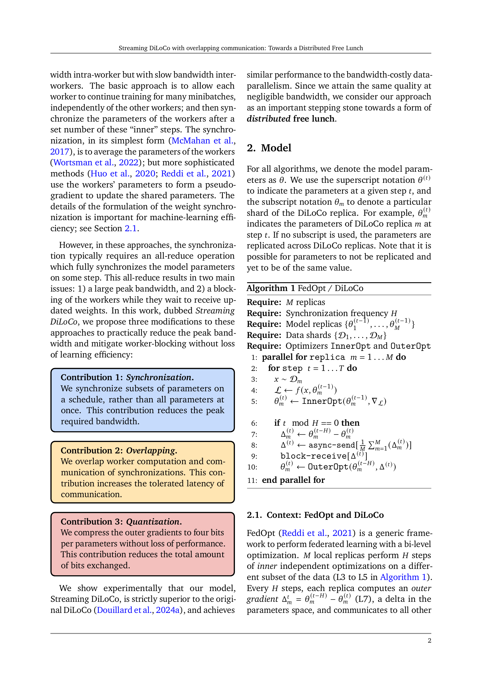
🔼 This figure illustrates two different methods for partitioning model parameters into fragments during training. The left panel depicts a sequential pattern where consecutive layers of the model are grouped into a single fragment. The right panel shows a strided pattern where layers are interleaved across different fragments. In both cases, only one fragment is synchronized at a time, improving communication efficiency by reducing the amount of data transferred during each synchronization step. The color-coding visually distinguishes different fragments within the model architecture. Each fragment is synchronized independently at a time, and different fragments get synchronized at each step.
read the caption
Figure 2: Streaming pattern: sequential (left) and strided (right). Colors denotes the fragment. A different fragment is synchronized each time.

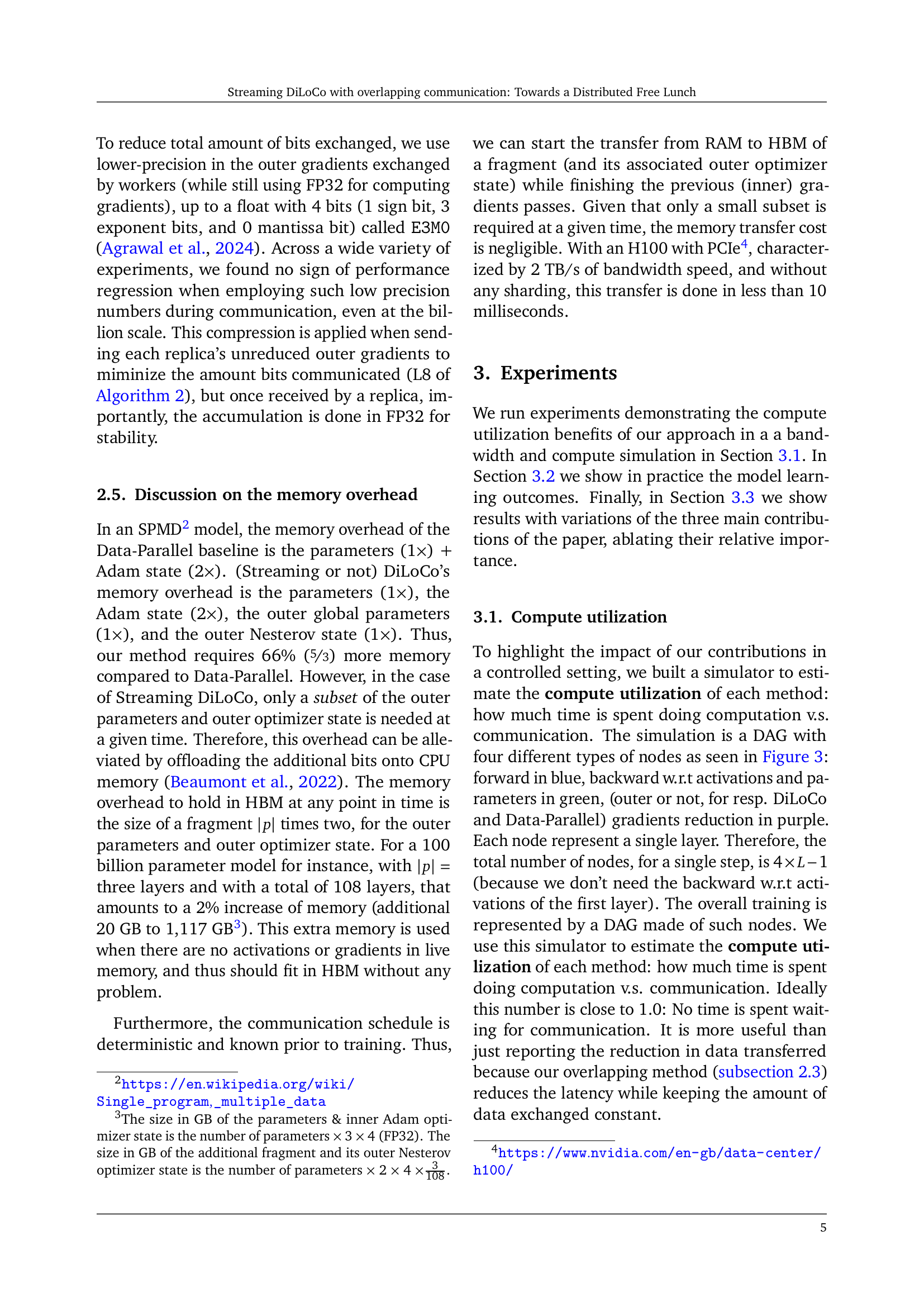
🔼 This figure displays a schedule where forward and backward passes are interleaved, along with outer gradient reduction. This interleaving is done for computation and communication overlap, a key technique in the paper. Forward passes are shown in blue, backward passes w.r.t. activations are in light green, backward passes w.r.t. parameters are in dark green, and gradient reduction is in purple. Each color represents a different stage in the process, and the interleaving helps to improve compute utilization by overlapping communication with computation.
read the caption
Figure 3: Simulation of a schedule interleaving forward passes (in blue), backward passes w.r.t. activations and parameters (resp. in light and dark green), and (outer) gradient reduction (in purple).

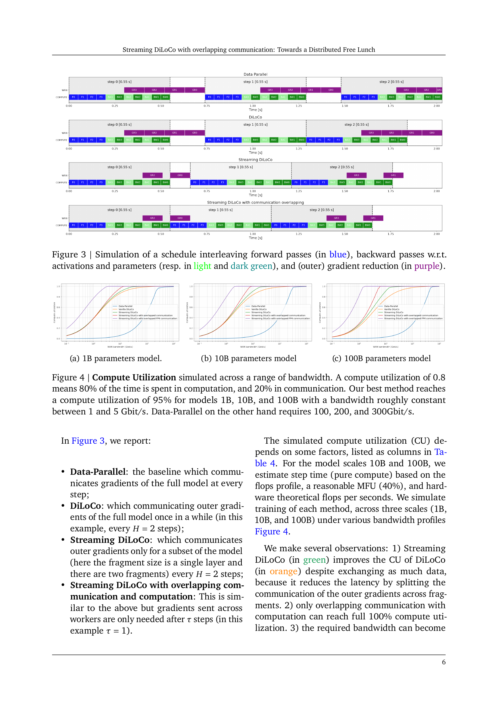
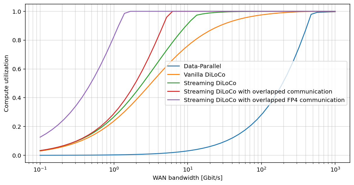
🔼 This figure shows the compute utilization simulated across a range of bandwidth for a model with 1 billion parameters. Compute utilization is a measure of the percentage of time spent on computation versus communication. A higher compute utilization indicates more efficient use of resources. The figure illustrates how the compute utilization varies as WAN (Wide Area Network) bandwidth increases. It also compares different methods (Data-Parallel, vanilla DiLoCo, Streaming DiLoCo, and Streaming DiLoCo with overlapping communication). This allows for an assessment of the communication efficiency of each method in relation to the available bandwidth. The graph shows that Streaming DiLoCo (with overlapping communication) has significantly higher compute utilization across the bandwidth range compared to the other methods, indicating that it uses resources more efficiently.
read the caption
(a) 1B parameters model.

🔼 This figure shows the compute utilization for a 10 billion parameter model across various bandwidths. Compute utilization is a measure of how much time is spent on actual computation versus communication. A higher compute utilization indicates better efficiency, with more time spent on productive computation and less time waiting for data transfer. The graph displays how the compute utilization improves as the available bandwidth increases, reaching nearly 95% utilization in the optimal bandwidth range.
read the caption
(b) 10B parameters model

🔼 This figure displays the compute utilization for a 100 billion parameter model across a range of bandwidth. Compute utilization is a measure of the percentage of time spent in computation versus communication. A higher compute utilization indicates that the model is spending more time performing computations and less time waiting for communication to complete. The graph shows how different methods (Data-Parallel, Vanilla DiLoCo, and variations of Streaming DiLoCo) achieve different compute utilization rates as the bandwidth changes.
read the caption
(c) 100B parameters model

🔼 This figure displays the compute utilization results for various deep learning model training methods across a range of bandwidths. Compute utilization represents the proportion of time dedicated to computation versus communication. A higher compute utilization indicates greater efficiency. The results show that the proposed ‘Streaming DiLoCo’ method achieves significantly higher compute utilization (approximately 95%) compared to the data-parallel baseline, especially at larger model sizes (1B, 10B, and 100B parameters). Importantly, Streaming DiLoCo achieves this high utilization with a considerably lower bandwidth (between 1 and 5 Gbit/s), whereas Data-Parallel requires much higher bandwidths (100, 200, and 300 Gbit/s). This demonstrates the effectiveness of Streaming DiLoCo in reducing communication overhead while maintaining computational efficiency.
read the caption
Figure 4: Compute Utilization simulated across a range of bandwidth. A compute utilization of 0.8 means 80% of the time is spent in computation, and 20% in communication. Our best method reaches a compute utilization of 95% for models 1B, 10B, and 100B with a bandwidth roughly constant between 1 and 5 Gbit/s. Data-Parallel on the other hand requires 100, 200, and 300Gbit/s.

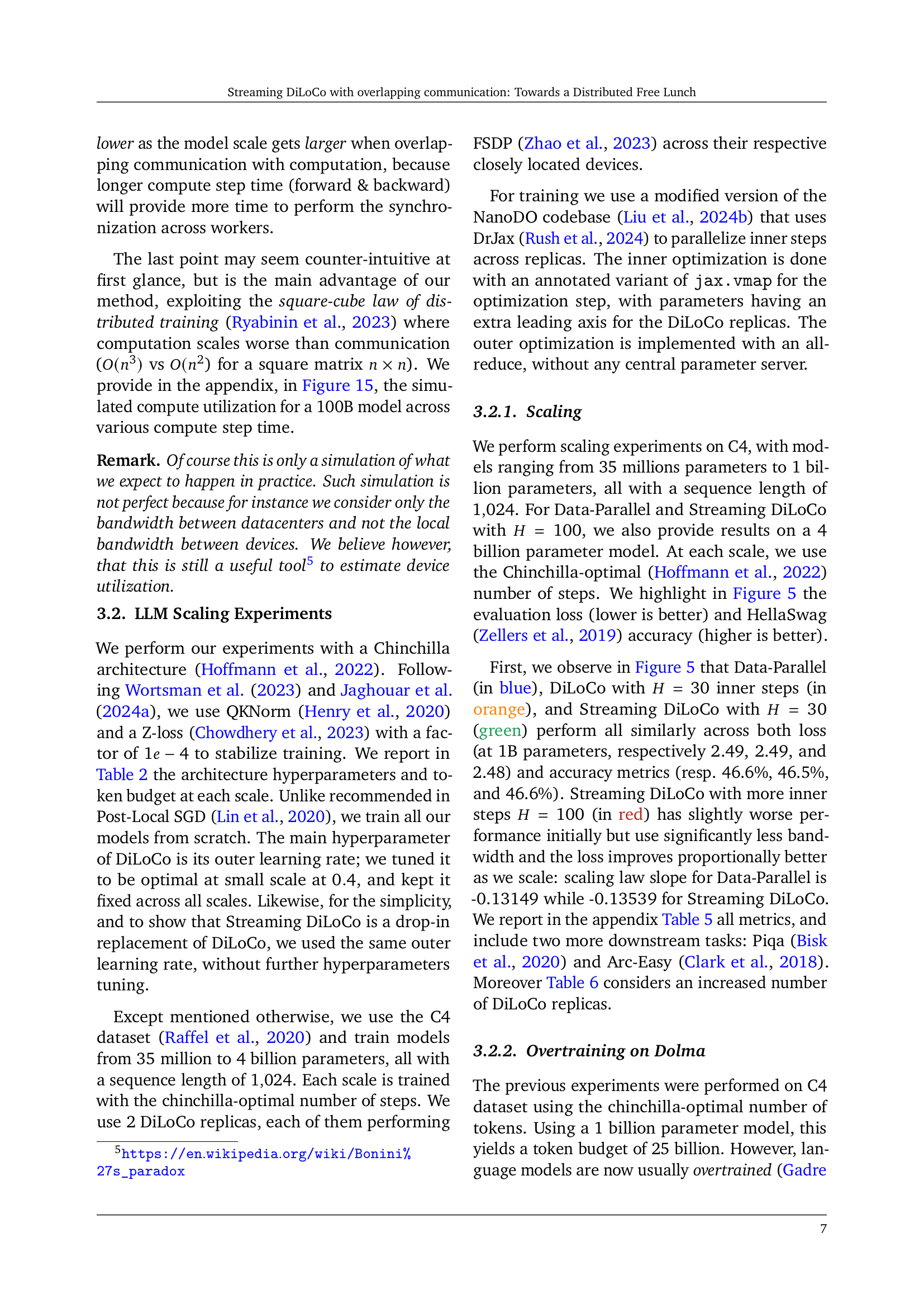
🔼 This figure shows the evaluation loss on the C4 dataset for different models and training methods. The x-axis represents the total number of training flops, and the y-axis shows the evaluation loss. It compares the performance of Data-Parallel, DiLoCo with 30 inner steps, Streaming DiLoCo with 30 inner steps, and Streaming DiLoCo with 100 inner steps across various model sizes. The plot visualizes how the loss decreases as the amount of computation (flops) increases for each method and illustrates the relative performance of each approach in large-scale language model training.
read the caption
(a) Evaluation loss on C4

🔼 This figure shows the HellaSwag accuracy for different compression methods applied to the outer gradients. It compares the performance using different levels of compression, including various forms of value dropping (FedDropout, Dare, and Top-k) and lower-precision floating-point numbers (fp4, fp8, and bf16). The x-axis represents the level of compression, and the y-axis shows the HellaSwag accuracy. The graph allows for the comparison of accuracy loss across different compression techniques and helps to determine the optimal trade-off between bandwidth reduction and model performance.
read the caption
(b) HellaSwag accuracy

🔼 This figure shows the results of scaling experiments on the C4 dataset, training language models with sizes ranging from 35 million parameters to 4 billion parameters. The x-axis represents the total number of training FLOPs (floating point operations), which is a measure of computational work. The y-axis of the left-hand plot shows the evaluation loss on the C4 dataset, while the y-axis of the right-hand plot shows the HellaSwag accuracy. Lower evaluation loss and higher HellaSwag accuracy indicate better model performance. The plot demonstrates how different methods (Data-Parallel, DiLoCo, and Streaming DiLoCo) perform as model size increases. It illustrates the scaling behavior and the relative performance of the methods.
read the caption
Figure 5: Scaling models from 35M (1.49e17 flops) to 4B parameters (2e21 flops) on C4.

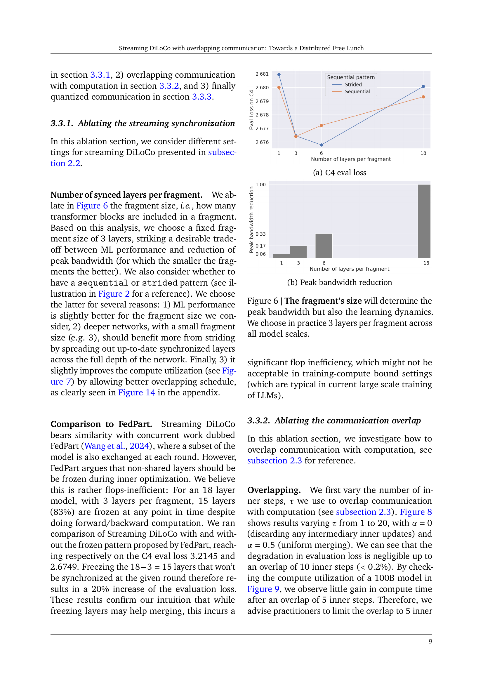
🔼 This figure shows the effect of varying the number of layers per fragment on the evaluation loss for the C4 dataset. The x-axis represents the number of layers per fragment, and the y-axis represents the evaluation loss. Two different fragment patterns (sequential and strided) are compared, showing the trade-off between performance and peak bandwidth reduction. The figure helps to determine the optimal fragment size for balancing these factors.
read the caption
(a) C4 eval loss
🔼 This figure shows the peak bandwidth reduction achieved by varying the fragment size in the Streaming DiLoCo model. Smaller fragment sizes lead to lower peak bandwidth requirements because synchronization happens more frequently, but on smaller subsets of parameters. The trade-off is explored, showing the impact of fragment size on bandwidth reduction.
read the caption
(b) Peak bandwidth reduction

🔼 This figure shows the effect of different fragment sizes on both peak bandwidth and model performance. The fragment size refers to the number of transformer blocks included in a single fragment during synchronization. Smaller fragment sizes reduce peak bandwidth but can impact learning dynamics. After experimentation across various model sizes, the authors determined that a fragment size of 3 layers provided an optimal balance between bandwidth efficiency and model performance. This size was consistently used across all model scales in subsequent experiments.
read the caption
Figure 6: The fragment’s size will determine the peak bandwidth but also the learning dynamics. We choose in practice 3 layers per fragment across all model scales.

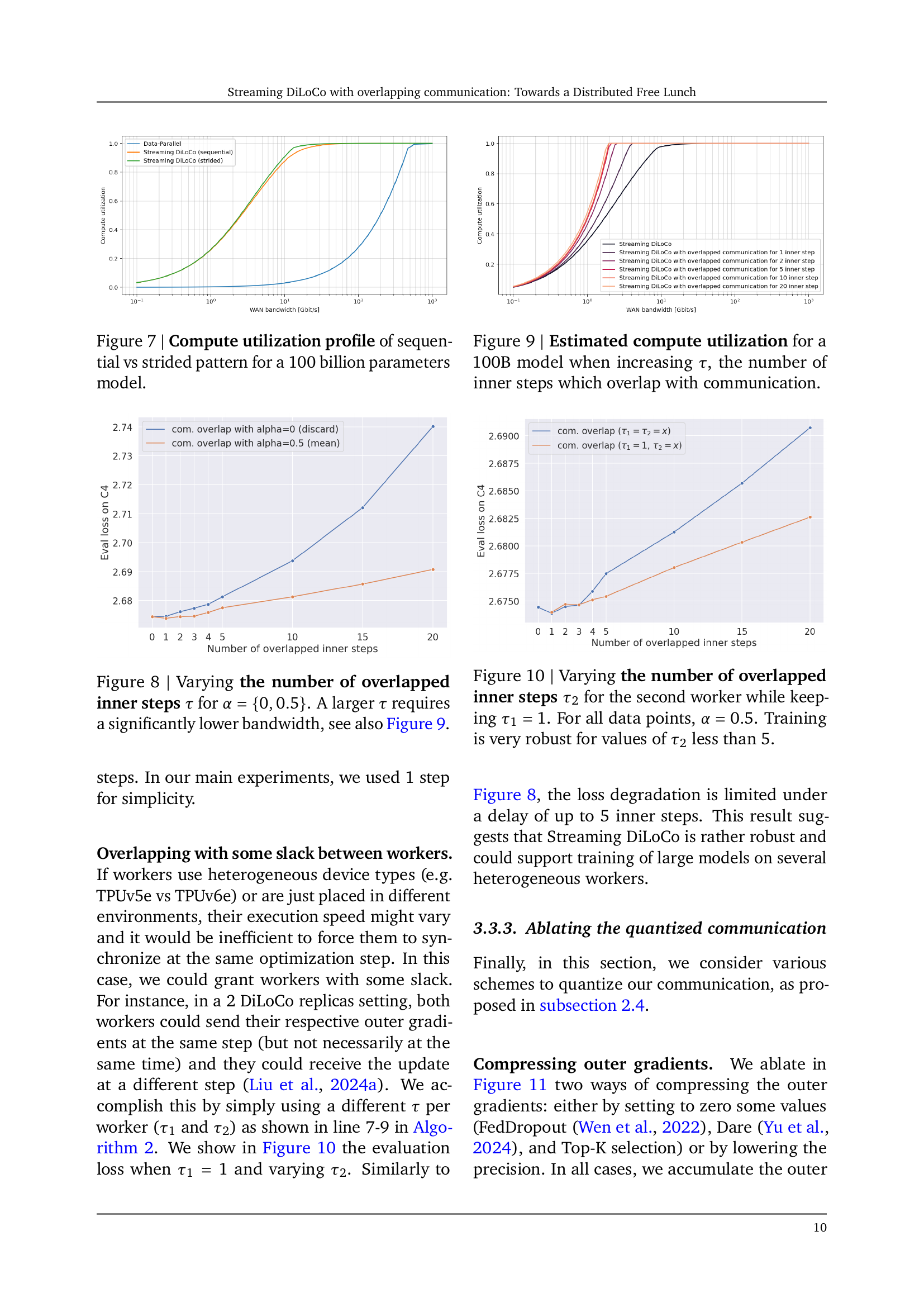
🔼 This figure compares the compute utilization of two different fragment patterns (sequential and strided) in the Streaming DiLoCo algorithm for a 100 billion parameter model. Compute utilization represents the percentage of time spent on computation versus communication. The x-axis represents the bandwidth, and the y-axis represents the compute utilization. The plot shows how compute utilization changes with varying bandwidth for both sequential and strided patterns. The strided pattern generally demonstrates better compute utilization, especially at higher bandwidths. This signifies that the strided fragment pattern leads to more efficient use of computing resources during training compared to the sequential pattern, particularly in bandwidth-rich environments.
read the caption
Figure 7: Compute utilization profile of sequential vs strided pattern for a 100 billion parameters model.

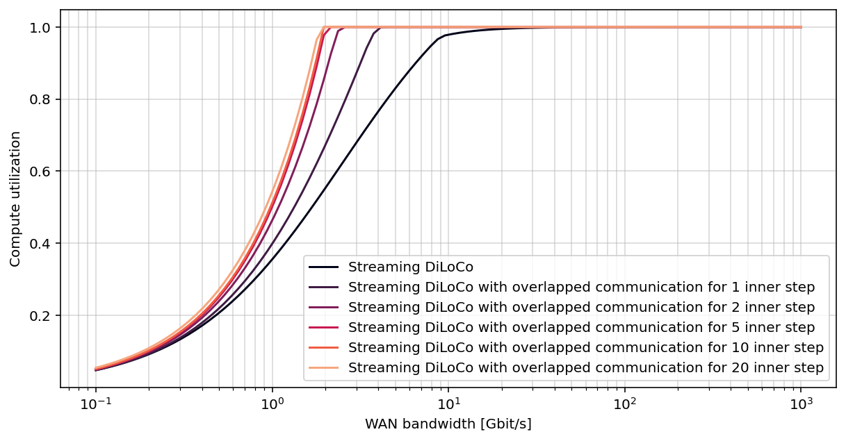
🔼 This figure shows the impact of varying the number of inner steps that overlap with communication (τ) on the model’s evaluation loss. Two scenarios are tested: α = 0 (no merging of local and global parameters) and α = 0.5 (averaging local and global parameters). The results show that increasing τ leads to a significant reduction in the required bandwidth for communication, as also shown in Figure 9.
read the caption
Figure 8: Varying the number of overlapped inner steps τ𝜏\tauitalic_τ for α={0,0.5}𝛼00.5\alpha=\{0,0.5\}italic_α = { 0 , 0.5 }. A larger τ𝜏\tauitalic_τ requires a significantly lower bandwidth, see also Figure 9.

🔼 This figure shows how compute utilization changes for a 100-billion parameter model as the number of inner optimization steps (τ) overlapped with communication increases. The x-axis represents the WAN bandwidth, and the y-axis represents the compute utilization. Different lines represent different numbers of overlapped steps (τ). The figure aims to demonstrate the impact of overlapping communication and computation on the efficiency of the training process by showing how much time is spent on computation vs. communication.
read the caption
Figure 9: Estimated compute utilization for a 100B model when increasing τ𝜏\tauitalic_τ, the number of inner steps which overlap with communication.
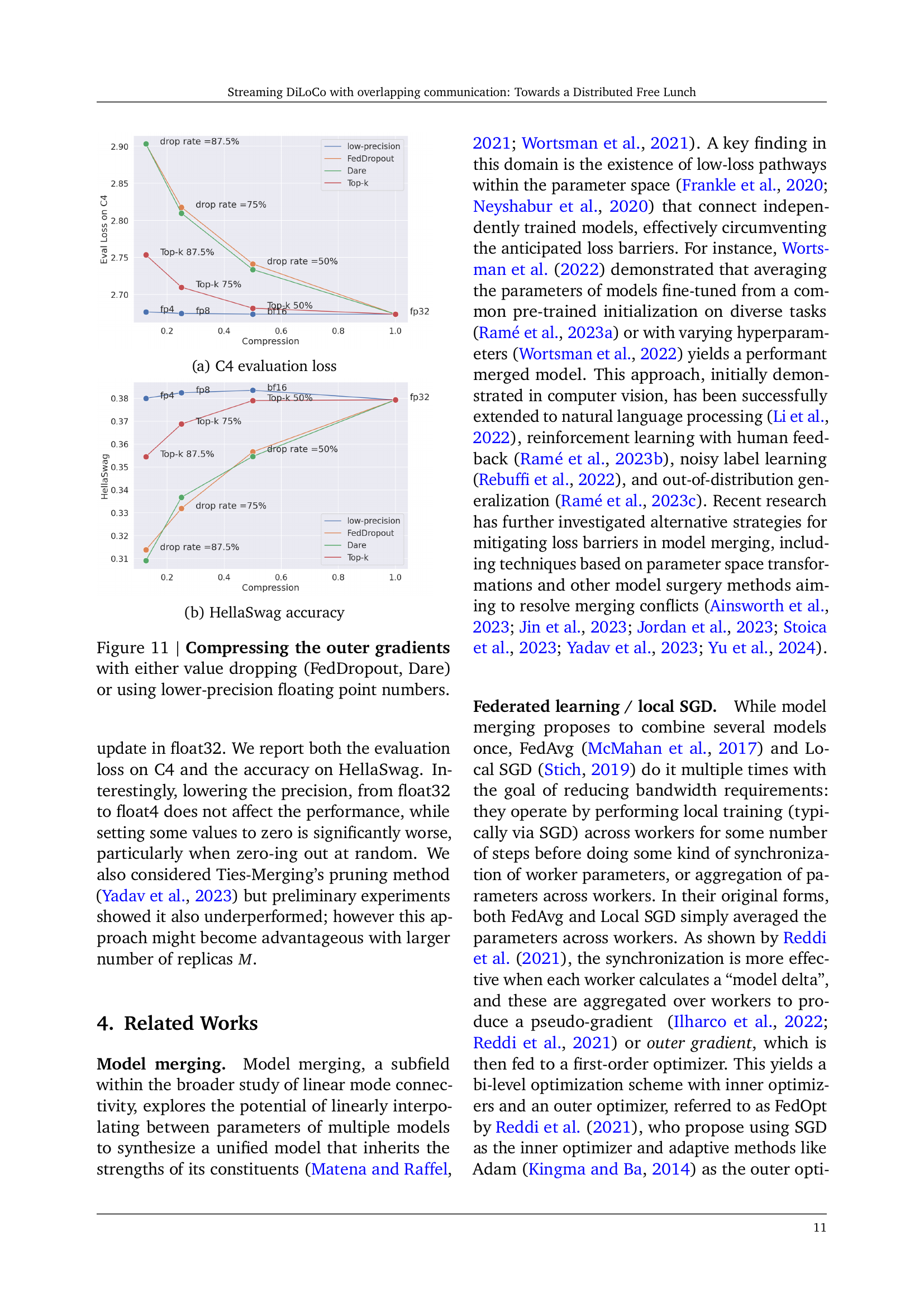
🔼 This figure shows the impact of overlapping communication with computation on model training. Specifically, it investigates how varying the number of inner steps (τ2) for the second worker, while keeping the number of inner steps for the first worker (τ1) constant at 1, affects the model’s loss. The alpha parameter (α) is set to 0.5, which represents a mean between using only locally computed updates and globally shared updates for parameter synchronization. The results demonstrate that the model’s performance (loss) is robust to increasing τ2, showing minimal degradation when τ2 is less than 5.
read the caption
Figure 10: Varying the number of overlapped inner steps τ2subscript𝜏2\tau_{2}italic_τ start_POSTSUBSCRIPT 2 end_POSTSUBSCRIPT for the second worker while keeping τ1=1subscript𝜏11\tau_{1}=1italic_τ start_POSTSUBSCRIPT 1 end_POSTSUBSCRIPT = 1. For all data points, α=0.5𝛼0.5\alpha=0.5italic_α = 0.5. Training is very robust for values of τ2subscript𝜏2\tau_{2}italic_τ start_POSTSUBSCRIPT 2 end_POSTSUBSCRIPT less than 5.

🔼 The figure shows the evaluation loss on the C4 dataset for various model sizes, ranging from 35 million to 4 billion parameters. Different training methods are compared: Data-Parallel, DiLoCo, and Streaming DiLoCo with different numbers of inner optimization steps (H) and inner communication overlap (τ). The x-axis represents the total number of training FLOPs, illustrating the scaling behavior of each method. The y-axis shows the evaluation loss, indicating the model’s performance in terms of prediction error.
read the caption
(a) C4 evaluation loss

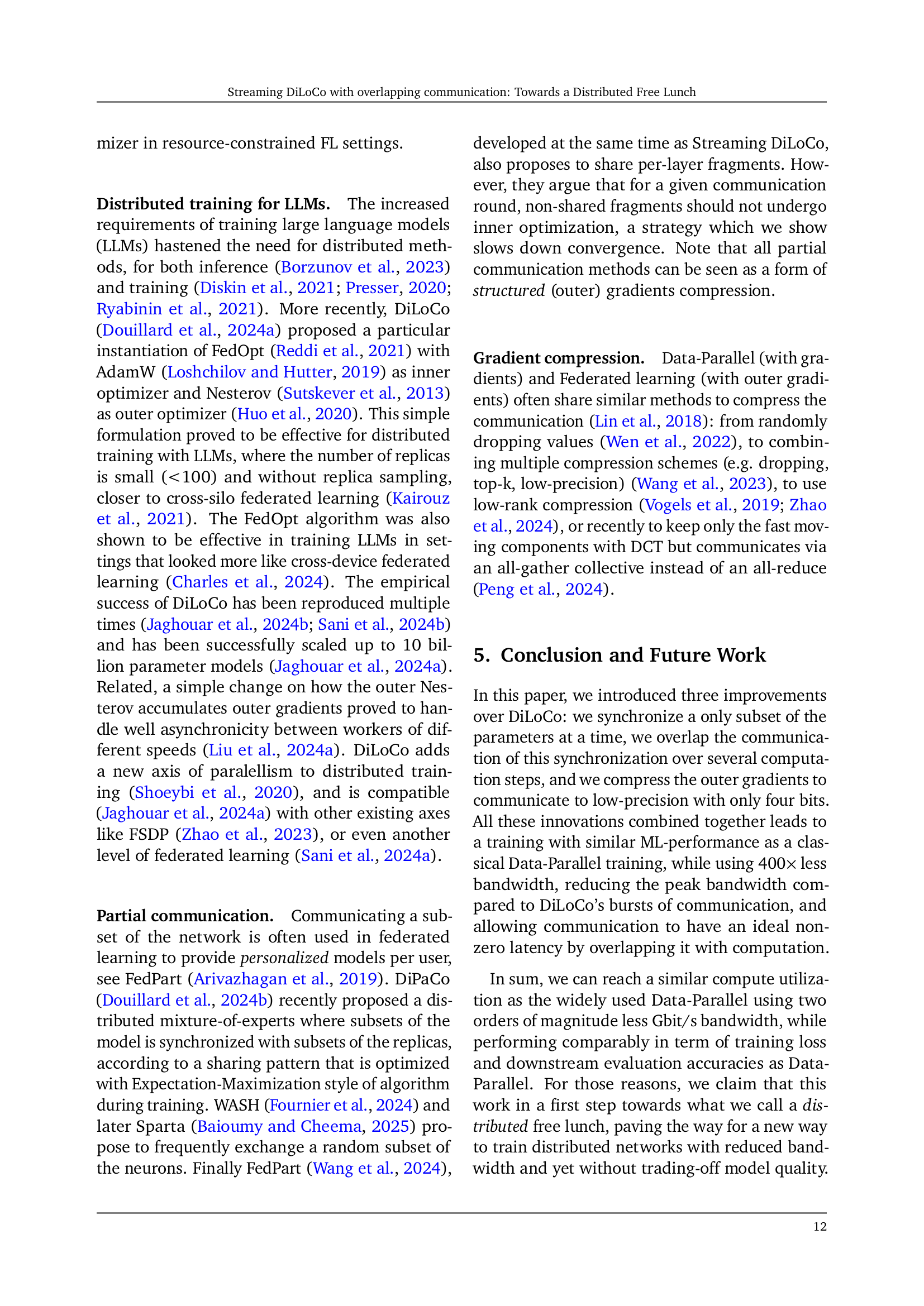
🔼 This figure shows the HellaSwag accuracy results for different compression methods applied to the outer gradients during communication. It compares the performance of using lower-precision floating-point numbers (fp4, fp8) and value-dropping methods (FedDropout, Dare, Top-k) to the baseline of using full-precision (fp32). The x-axis represents the compression rate, and the y-axis represents the HellaSwag accuracy. The results indicate the impact of different compression techniques on the model’s performance in a downstream task, demonstrating that reducing the precision of communication does not significantly affect accuracy at the billion-scale parameter model size.
read the caption
(b) HellaSwag accuracy
🔼 This figure displays the results of ablating the effect of compressing outer gradients by either dropping values (using FedDropout and Dare methods) or using lower-precision floating point numbers (FP4, FP8, BF16). The left panel shows the evaluation loss on the C4 dataset, while the right panel displays the HellaSwag accuracy. The different compression techniques are compared against the baseline of using full-precision (FP32) numbers to highlight the impact of compression on both loss and accuracy.
read the caption
Figure 11: Compressing the outer gradients with either value dropping (FedDropout, Dare) or using lower-precision floating point numbers.

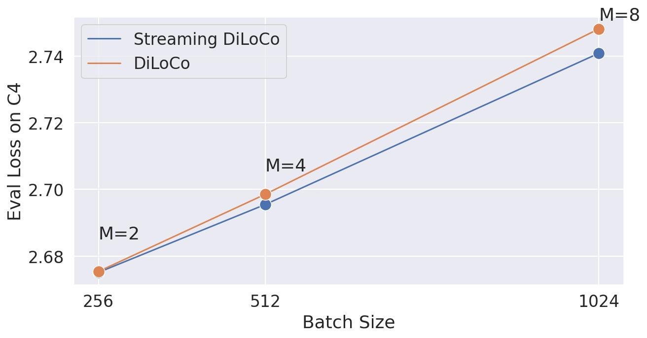
🔼 This figure shows the impact of varying the number of replicas on the evaluation loss, while keeping the global batch size constant. As the number of replicas increases, the local per-replica batch size decreases. This experiment helps to understand the effect of the local batch size on model performance in a distributed training setting. The x-axis shows the number of replicas, and the y-axis represents the evaluation loss on the C4 dataset. Two lines are shown, one for Streaming DiLoCo and one for DiLoCo, illustrating the performance difference between the two methods.
read the caption
(a) Keeping the global batch size constant, and thus decreasing the local per-replica batch size.

🔼 This figure shows the effect of scaling the number of replicas while keeping the local batch size constant. Increasing the number of replicas leads to a larger global batch size. The experiment demonstrates how the evaluation loss on C4 changes with the increase in the number of replicas, while maintaining a consistent local batch size. This visualization helps analyze the impact of distributed training on model performance under different scaling scenarios.
read the caption
(b) Keeping the local per-replica batch size constant, and thus increasing the global batch size.

🔼 This figure shows the impact of increasing the number of DiLoCo replicas while keeping the total token budget constant. It consists of two subfigures. Subfigure (a) keeps the global batch size constant and reduces the local per-replica batch size as the number of replicas increases, while subfigure (b) keeps the local per-replica batch size constant and increases the global batch size. Both subfigures compare the performance of DiLoCo and Streaming DiLoCo under these different scaling scenarios.
read the caption
Figure 12: Scaling the number of DiLoCo replicas M𝑀Mitalic_M from M=2𝑀2M=2italic_M = 2 to M=4𝑀4M=4italic_M = 4. For all experiments, the token budget is kept constant.

🔼 This figure shows the effect of changing the number of inner steps (H) in DiLoCo and Streaming DiLoCo on the evaluation loss. The total number of training steps is kept constant, so reducing H increases the number of communication rounds. The results demonstrate the trade-off between communication cost and model performance. A lower H implies more frequent communication but may also result in noisy gradient updates, while a higher H reduces the communication frequency but increases the risk of replicas drifting apart.
read the caption
Figure 13: Varying the number of inner steps H𝐻Hitalic_H for DiLoCo and Streaming DiLoCo while keeping the total number of steps constants. A lower H𝐻Hitalic_H means more communication rounds to be done.

🔼 This figure visualizes the scheduling of computations and communication in Streaming DiLoCo, comparing sequential and strided fragment patterns. The blue bars represent forward passes, light and dark green bars represent backward passes (w.r.t. activations and weights, respectively), and purple bars represent outer gradient reduction. The illustration shows how computations and communication are interleaved, allowing for overlapping and improved efficiency. The difference in scheduling between sequential and strided fragments highlights the impact of the chosen strategy on resource utilization.
read the caption
Figure 14: Simulation of a schedule interleaving forward passes (in blue), backward passes w.r.t. activations and weights (resp. in light and dark green), and (outer) gradient reduction (in purple) for Streaming DiLoCo, respectively with a sequential and strided pattern.

🔼 This figure shows the compute utilization for a 100 billion parameters model when the computation time for one step is set to 1 second. Compute utilization represents the percentage of time spent on computation versus communication. The graph displays compute utilization across a range of bandwidth, highlighting the impact of different optimization methods. Data-parallel, vanilla DiLoCo, and various streaming DiLoCo methods are compared to show the efficiency gains achieved by overlapping communication with computation and using lower-precision gradients.
read the caption
(a) 1s step time
More on tables
| Model scale | Hidden dim | Num layers | Num heads | Token budget |
|---|---|---|---|---|
| 35M | 6 | 8 | 700M | |
| 100M | 9 | 12 | 1.5B | |
| 200M | 12 | 16 | 3.5B | |
| 300M | 15 | 20 | 6B | |
| 500M | 18 | 24 | 11B | |
| 1B | 24 | 32 | 25B | |
| 4B | 36 | 48 | 83B |
🔼 This table lists the architecture hyperparameters for language models of various sizes, ranging from 35 million to 4 billion parameters. For each model size, it shows the hidden dimension, number of layers, number of attention heads, and the corresponding chinchilla-optimal token budget. The vocabulary size is consistent across all models at 32,000.
read the caption
Table 2: Architecture hyperparameters: we consider model from 35M to 4B with the following hyperameters and chinchilla-optimal token budget. For all model scale, the vocabulary size is 32,0003200032{,}00032 , 000.
| Parameters evaluated | Eval Loss | HellaSwag |
|---|---|---|
| First replica | 2.77 | 37.77 |
| Replicas average | 2.68 | 37.72 |
| Outer parameters | 2.67 | 37.78 |
🔼 This table compares the performance of using different sets of model parameters for training. The three methods compared are using parameters from only the first replica, averaging parameters across all replicas, and using only the outer (globally shared) parameters. The outer parameters are updated less frequently than the inner parameters. The results show that using only the outer parameters leads to the best performance, suggesting that less-frequent synchronization on only a subset of parameters is beneficial.
read the caption
Table 3: Which parameters to evaluate?: Evaluating the outer parameters, where each fragment has been synchronized at a different moment in time, yields better performance than any inner parameters.
| Model size | # layers | Step time | Method | Gbit/s to reach a compute utilization ? | ||||
|---|---|---|---|---|---|---|---|---|
| 1B | 24 | 0.1s | Data-Parallel | 86.8 | 152.6 | 184.2 | 222.3 | 569.0 |
| Vanilla DiLoCo | 1.4 | 6.2 | 13.3 | 23.3 | 86.8 | |||
| Streaming DiLoCo | 1.4 | 5.2 | 9.1 | 16.0 | 28.1 | |||
| Streaming DiLoCo w/ overlapped com. | 1.4 | 4.3 | 6.2 | 9.1 | 11.0 | |||
| Streaming DiLoCo w/ overlapped FP4 com. | 0.4 | 0.9 | 1.7 | 2.0 | 3.0 | |||
| 10B | 48 | 0.8s | Data-Parallel | 104.8 | 222.3 | 222.3 | 268.3 | 471.5 |
| Vanilla DiLoCo | 1.7 | 7.5 | 16.0 | 33.9 | 104.8 | |||
| Streaming DiLoCo | 1.7 | 5.2 | 9.1 | 13.3 | 19.3 | |||
| Streaming DiLoCo w/ overlapped com. | 1.7 | 3.6 | 5.2 | 6.2 | 7.5 | |||
| Streaming DiLoCo w/ overlapped FP4 com. | 0.4 | 0.9 | 1.4 | 1.4 | 1.7 | |||
| 100B | 108 | 4.9s | Data-Parallel | 184.2 | 323.8 | 390.7 | 390.7 | 471.5 |
| Vanilla DiLoCo | 3.0 | 11.0 | 23.3 | 49.4 | 184.2 | |||
| Streaming DiLoCo | 2.4 | 6.2 | 9.1 | 11.0 | 19.3 | |||
| Streaming DiLoCo w/ overlapped com. | 1.7 | 3.6 | 4.3 | 5.2 | 5.2 | |||
| Streaming DiLoCo w/ overlapped FP4 com. | 0.5 | 0.9 | 1.1 | 1.1 | 1.4 | |||
🔼 This table presents a simulation of compute utilization for different model training methods across various bandwidths. It estimates the time spent in computation versus communication for Data-Parallel, DiLoCo, and different variations of Streaming DiLoCo. The simulation considers 10B and 100B parameter models, using the FLOPS profile from Kaplan et al. (2020) and a machine utilization factor (MFU) of 60%. The DiLoCo and Streaming DiLoCo methods use a synchronization frequency (H) of 100 and Streaming DiLoCo variations use a fragment size of 3 layers. The goal is to illustrate how the proposed modifications reduce the bandwidth requirements while maintaining compute efficiency.
read the caption
Table 4: Simulation: we estimate the step time (pure compute) of 10B and 100B based on the required flops using Kaplan et al. (2020) rule and using a MFU of 60%. For all DiLoCo and Streaming DiLoCo-variants, we use H=100𝐻100H=100italic_H = 100. For all Streaming DiLoCo-variants, we use a fragment size of 3 layers.
| Model size | Flops | Method | Eval Loss | HellaSwag | Piqa | Arc Easy |
|---|---|---|---|---|---|---|
| 35M | 1.5e17 | Data-Parallel | 3.51 | 24.62 | 57.89 | 29.65 |
| DiLoCo H=30 | 3.54 | 24.53 | 58.11 | 29.65 | ||
| Streaming DiLoCo with overlapped FP4 com., H=30 | 3.53 | 24.46 | 57.67 | 30.53 | ||
| Streaming DiLoCo with overlapped FP4 com., H=100 | 3.56 | 24.80 | 57.89 | 29.12 | ||
| 100M | 9.4e17 | Data-Parallel | 3.19 | 26.94 | 60.12 | 30.35 |
| DiLoCo H=30 | 3.21 | 26.59 | 60.50 | 29.12 | ||
| Streaming DiLoCo with overlapped FP4 com., H=30 | 3.21 | 26.97 | 59.58 | 31.40 | ||
| Streaming DiLoCo with overlapped FP4 com., H=100 | 3.22 | 26.68 | 60.39 | 31.93 | ||
| 200M | 4e18 | Data-Parallel | 2.97 | 29.86 | 63.71 | 35.44 |
| DiLoCo H=30 | 2.98 | 29.71 | 62.30 | 33.68 | ||
| Streaming DiLoCo with overlapped FP4 com., H=30 | 2.98 | 29.67 | 61.92 | 34.39 | ||
| Streaming DiLoCo with overlapped FP4 com., H=100 | 3.00 | 29.27 | 62.13 | 34.21 | ||
| 300M | 1.4e19 | Data-Parallel | 2.80 | 33.46 | 64.69 | 34.91 |
| DiLoCo H=30 | 2.81 | 33.87 | 64.74 | 34.74 | ||
| Streaming DiLoCo with overlapped FP4 com., H=30 | 2.81 | 33.66 | 63.49 | 35.09 | ||
| Streaming DiLoCo with overlapped FP4 com., H=100 | 2.83 | 33.00 | 63.71 | 34.39 | ||
| 500M | 4.7e19 | Data-Parallel | 2.67 | 38.68 | 66.49 | 37.19 |
| DiLoCo H=30 | 2.68 | 38.37 | 65.61 | 36.32 | ||
| Streaming DiLoCo with overlapped FP4 com., H=30 | 2.67 | 38.10 | 66.21 | 34.91 | ||
| Streaming DiLoCo with overlapped FP4 com., H=100 | 2.69 | 37.40 | 65.51 | 34.74 | ||
| 1B | 1.9e20 | Data-Parallel | 2.49 | 46.60 | 68.93 | 39.65 |
| DiLoCo H=30 | 2.49 | 46.56 | 68.82 | 36.84 | ||
| Streaming DiLoCo with overlapped FP4 com., H=30 | 2.48 | 46.60 | 69.04 | 39.12 | ||
| Streaming DiLoCo with overlapped FP4 com., H=100 | 2.50 | 46.00 | 68.82 | 38.42 | ||
| 4B | 2e21 | Data-Parallel | 2.25 | 59.56 | 72.42 | 43.51 |
| DiLoCo H=30 | - | - | - | - | ||
| Streaming DiLoCo with overlapped FP4 com., H=30 | - | - | - | - | ||
| Streaming DiLoCo with overlapped FP4 com., H=100 | 2.26 | 59.02 | 72.52 | 43.16 |
🔼 This table presents the results of scaling experiments on language models with varying numbers of parameters (from 35 million to 4 billion). The models were trained using a chinchilla-optimal number of floating point operations, and the evaluation loss on the validation set of the C4 dataset is reported for each model size.
read the caption
Table 5: Scaling from 35 million parameters to 4 billion parameters using a chinchilla-optimal number of flops/tokens. We train on the C4 dataset, and report the evaluation loss on its validation set.
| Model size | Flops | Eval Loss | HellaSwag | Piqa | Arc Easy | ||
|---|---|---|---|---|---|---|---|
| 35M | 1.5e17 | 2 | 30 | 3.53 | 24.46 | 57.67 | 30.53 |
| 4 | 30 | 3.60 | 24.50 | 56.09 | 28.60 | ||
| 2 | 100 | 3.56 | 24.80 | 57.89 | 29.12 | ||
| 4 | 100 | 3.64 | 24.67 | 56.75 | 26.84 | ||
| 100M | 9.4e17 | 2 | 30 | 3.21 | 26.97 | 59.58 | 31.40 |
| 4 | 30 | 3.25 | 26.24 | 59.74 | 32.63 | ||
| 2 | 100 | 3.22 | 26.68 | 60.39 | 31.93 | ||
| 4 | 100 | 3.29 | 26.54 | 60.34 | 29.82 | ||
| 200M | 4e18 | 2 | 30 | 2.98 | 29.67 | 61.92 | 34.39 |
| 4 | 30 | 3.02 | 29.09 | 62.89 | 35.44 | ||
| 2 | 100 | 3.00 | 29.27 | 62.13 | 34.21 | ||
| 4 | 100 | 3.05 | 28.53 | 61.10 | 33.51 | ||
| 300M | 1.4e19 | 2 | 30 | 2.81 | 33.66 | 63.49 | 35.09 |
| 4 | 30 | 2.84 | 32.54 | 64.42 | 34.74 | ||
| 2 | 100 | 2.83 | 33.00 | 63.71 | 34.39 | ||
| 4 | 100 | 2.87 | 32.02 | 64.25 | 35.44 | ||
| 500M | 4.7e19 | 2 | 30 | 2.67 | 38.10 | 66.21 | 34.91 |
| 4 | 30 | 2.70 | 36.95 | 65.72 | 35.26 | ||
| 2 | 100 | 2.69 | 37.40 | 65.51 | 34.74 | ||
| 4 | 100 | 2.73 | 36.02 | 66.27 | 35.09 | ||
| 1B | 1.9e20 | 2 | 30 | 2.48 | 46.60 | 69.04 | 39.12 |
| 4 | 30 | 2.50 | 45.25 | 67.95 | 39.12 | ||
| 2 | 100 | 2.50 | 46.00 | 68.82 | 38.42 | ||
| 4 | 100 | 2.53 | 44.74 | 68.34 | 38.25 |
🔼 This table presents the results of scaling experiments using Streaming DiLoCo, a distributed training method for large language models. The experiments vary the model size from 35 million to 1 billion parameters, while also altering two key hyperparameters: the synchronization frequency (H), which determines how often parameters are synchronized across workers, and the number of DiLoCo replicas (M), which represents the degree of parallelism. The table shows how the model’s performance (evaluation loss, HellaSwag accuracy, Piqa accuracy, and Arc Easy accuracy) changes across these different configurations. The use of overlapped FP4 (four-bit floating point) communication is consistent across all experiments.
read the caption
Table 6: Scaling from 35 million parameters to 1 billion parameters Streaming DiLoCo with overlapped FP4 communication and with two different synchronization frequencies H={30,100}𝐻30100H=\{30,100\}italic_H = { 30 , 100 } and number of DiLoCo replicas M={2,4}.𝑀24M=\{2,4\}.italic_M = { 2 , 4 } .
| Method | Token Budget | Terabytes exchanged | Eval Loss | HellaSwag | Piqa | Arc Easy |
|---|---|---|---|---|---|---|
| Data-Parallel | 25B | 441 | 2.67 | 42.09 | 67.35 | 40.42 |
| 100B | 1,767 | 2.52 | 49.78 | 69.15 | 44.03 | |
| 250B | 4,418 | 2.45 | 53.86 | 70.45 | 44.21 | |
| Our method, M=2 | 25B | 1.10 | 2.66 | 42.08 | 67.46 | 38.42 |
| 100B | 4.42 | 2.51 | 49.98 | 69.96 | 44.03 | |
| 250B | 11.05 | 2.45 | 54.24 | 71.38 | 41.92 | |
| Our method, M=4 | 25B | 0.55 | 2.73 | 38.93 | 66.92 | 39.64 |
| 100B | 2.21 | 2.54 | 48.35 | 69.42 | 40.52 | |
| 250B | 5.52 | 2.47 | 52.20 | 70.29 | 42.45 |
🔼 This table presents the results of overtraining experiments conducted on the Dolma dataset using a 1-billion parameter model. The experiments varied the token budget (25B, 100B, and 250B tokens) and the number of DiLoCo replicas (M=2 and M=4). Doubling the number of replicas doubles the global batch size while halving the number of training steps. This leads to approximately twice the training speed, although at a slight cost to performance. The table shows that Streaming DiLoCo with overlapped FP4 communication, the method proposed in this paper, achieves competitive performance.
read the caption
Table 7: Overtraining on the Dolma dataset with a 1 billion parameters model, and with an increasing token budgets (25B, 100B, and 250B). We report here for our model both with M=2𝑀2M=2italic_M = 2 and M=4𝑀4M=4italic_M = 4 DiLoCo replicas. With twice more replicas, the global batch size is doubled, and twice less steps are done. It is also thus roughly twice faster, but come with slightly worse performance. Our method is the final model: Streaming DiLoCo with overlapped FP4 communication.
Full paper#