TL;DR#
Standard Transformer models suffer from representation collapse, where lengthy sequences lead to loss of subtle information due to compression within each layer’s single residual stream. This limits their ability to capture complex patterns and achieve optimal performance. The issue is particularly pronounced when dealing with long sequences or tasks requiring fine-grained distinctions between similar inputs.
To tackle this problem, researchers propose Layer-Integrated Memory (LIMe), a method that expands the model’s representational capacity while maintaining its overall memory footprint. LIMe allows access to hidden states from previous layers through a learned routing mechanism. Extensive experiments across diverse architectures and lookup mechanisms demonstrate LIMe’s consistent performance improvements. Analyses reveal how LIMe efficiently integrates information across layers, suggesting promising research directions for building deeper and more robust Transformer models.
Key Takeaways#
Why does it matter?#
This paper is crucial because it addresses the critical issue of representation collapse in Transformer models, a significant limitation hindering progress in various AI applications. By introducing a novel solution, LIMe, it offers significant performance improvements and unveils new avenues for building deeper and more robust Transformer models. This is directly relevant to the current push for more efficient and effective large language models, making it highly significant for researchers in the field.
Visual Insights#

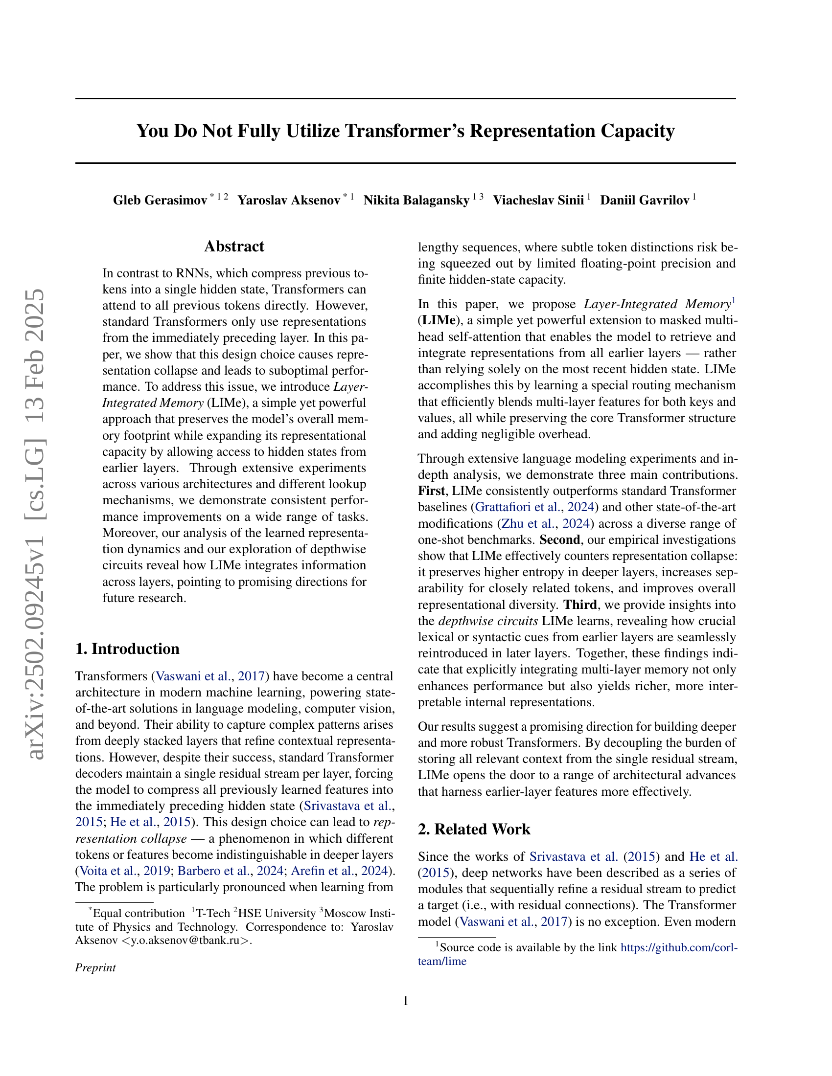
🔼 The figure shows the training loss as a function of FLOPs (floating point operations) for three different language models: Llama, Static LIMe, and Dynamic LIMe. FLOPs are a measure of computational cost. The plot demonstrates that both Static LIMe and Dynamic LIMe achieve significantly lower training loss compared to Llama, while maintaining a similar level of computational cost (FLOPs). This indicates that LIMe, a modification to the standard transformer architecture, improves training efficiency by better utilizing the model’s representational capacity.
read the caption
Figure 1: Training loss per FLOPs for Llama, Static LIMe, and Dynamic LIMe. LIMe has a substantially lower loss with a similar amount of FLOPs. See Section 5.1 for more details.
| Model | ARC-E | ARC-C | Winogrande | COPA | MultiRC | RTE | HellaSwag | PIQA | Avg |
|---|---|---|---|---|---|---|---|---|---|
| LLaMA | 69.5 | 38.7 | 55.2 | 75.0 | 42.8 | 54.5 | 53.1 | 72.5 | 57.7 |
| HC | 70.1 | 38.4 | 53.0 | 77.0 | 42.9 | 51.6 | 54.4 | 73.5 | 57.6 |
| LIMe Dynamic | 72.7 | 39.5 | 53.1 | 79.0 | 43.0 | 52.4 | 54.4 | 72.9 | 58.4 |
| LIMe Static | 71.1 | 39.3 | 56.2 | 75.0 | 43.1 | 55.2 | 53.9 | 72.2 | 58.3 |
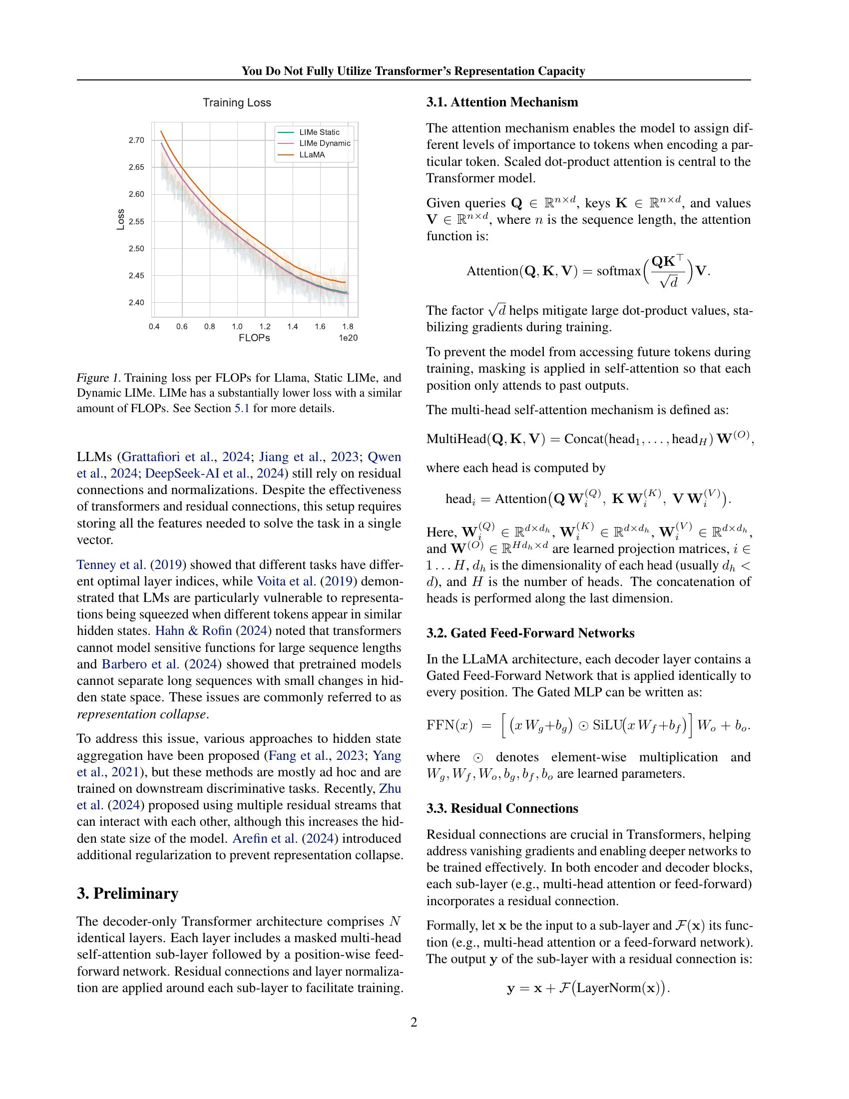
🔼 This table presents the results of several language models on the LM Evaluation Harness benchmark. The models compared are LLaMA, HyperConnections, LIMe Static, and LIMe Dynamic, all with approximately 1.2 billion parameters. The benchmark evaluates performance across various tasks using only one example per task (num-fewshots=1). The table shows the accuracy (in percentage) for each model on each task. The final column presents the average accuracy across all tasks, demonstrating that the proposed LIMe methods (LIMe Static and LIMe Dynamic) outperform the baselines (LLaMA and HyperConnections).
read the caption
Table 1: LM Evaluation Harness benchmarks (accuracies in %) on 1.2B models with num-fewshots 1. The rightmost column shows average accuracy across the tasks. Proposed methods outperform both LLaMA and HyperConnections (Zhu et al., 2024) baselines. See Section 5.1 for more details.
In-depth insights#
Transformer Limits#
Transformer limitations primarily stem from their inherent architecture. While highly effective at capturing long-range dependencies, the reliance on self-attention mechanisms leads to computational costs that scale quadratically with sequence length. Memory limitations restrict the length of sequences that can be effectively processed. Furthermore, representational collapse, where distinct input tokens become indistinguishable in deeper layers, can significantly hinder performance. Training instability is another concern, particularly in very deep models. Finally, the inherent difficulty in interpreting the internal representations learned by Transformers poses a challenge for understanding their decision-making processes and improving model interpretability.
LIMe: Multi-Layer#
The proposed LIMe (Layer-Integrated Memory) model introduces a novel multi-layer approach to Transformer architecture. Instead of relying solely on the previous layer’s representations, LIMe incorporates information from all preceding layers, enriching the contextual understanding and mitigating representation collapse. This is achieved through a learnable router mechanism that efficiently combines multi-layer features for both keys and values in the self-attention mechanism. The method’s effectiveness stems from its ability to prevent information squishing and preserve crucial details across layers. LIMe’s dynamic router offers even greater flexibility by allowing per-token adaptation of the information blend, leading to improved performance and richer, more interpretable internal representations. By decoupling context storage from the single residual stream, LIMe unlocks the potential for building deeper and more robust Transformers, opening new avenues for architectural innovations that exploit the full representational capacity of the model.
Representation Gain#
The concept of “Representation Gain” in the context of the provided research paper likely refers to the performance improvements achieved by enhancing the model’s ability to represent information. The paper likely demonstrates that standard transformers underutilize their representational capacity by focusing solely on the immediately preceding layer’s hidden states. The proposed LIMe method directly addresses this limitation by introducing a mechanism that allows the model to access and integrate information from earlier layers, effectively expanding its representational capacity. This leads to improved performance across various tasks, as shown in the experimental results. The key to the representation gain lies in the mitigation of representation collapse, a phenomenon where distinct features become indistinguishable in deeper layers due to information compression. By leveraging multi-layer memory, LIMe preserves higher entropy and enhances overall representation diversity, resulting in significantly improved model performance.
Depthwise Circuits#
The concept of “Depthwise Circuits” in the context of a Transformer-based language model suggests an examination of how information flows and is processed across different layers. It implies a focus on the specific pathways of information, rather than just the overall transformation. Analyzing depthwise circuits could reveal crucial insights into how the model learns and integrates information from earlier layers, leading to improved performance. Identifying recurring patterns within these circuits could unveil the model’s underlying decision-making processes, providing interpretability. The analysis might reveal specialized circuits for handling specific linguistic features such as morphology or syntax. For example, a circuit might be dedicated to processing morphological information from early layers or syntactic relationships across multiple layers. This approach helps uncover how a Transformer model leverages its multi-layered structure for effective information integration.
Future: Deeper LMs#
The prospect of “Future: Deeper LMs” is exciting yet challenging. The success of current large language models (LLMs) hinges on their scale, but simply increasing depth isn’t a guaranteed path to improvement. Representation collapse, where subtle distinctions between tokens are lost in deeper layers, is a significant hurdle. Addressing this requires innovative architectural solutions beyond simply stacking more layers. Methods like LIMe, which explicitly integrate information from earlier layers, offer a promising direction. However, even with such methods, memory and computational costs increase exponentially with depth. Strategies to mitigate this are crucial, including exploring more efficient attention mechanisms, advanced pruning techniques, and potentially, novel training paradigms. Ultimately, the future of deeper LMs depends on finding a balance between enhanced representation capacity, manageable resource requirements, and interpretability.
More visual insights#
More on figures
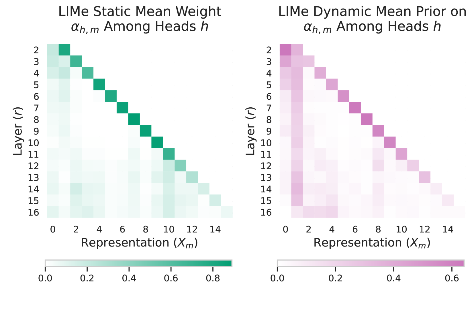
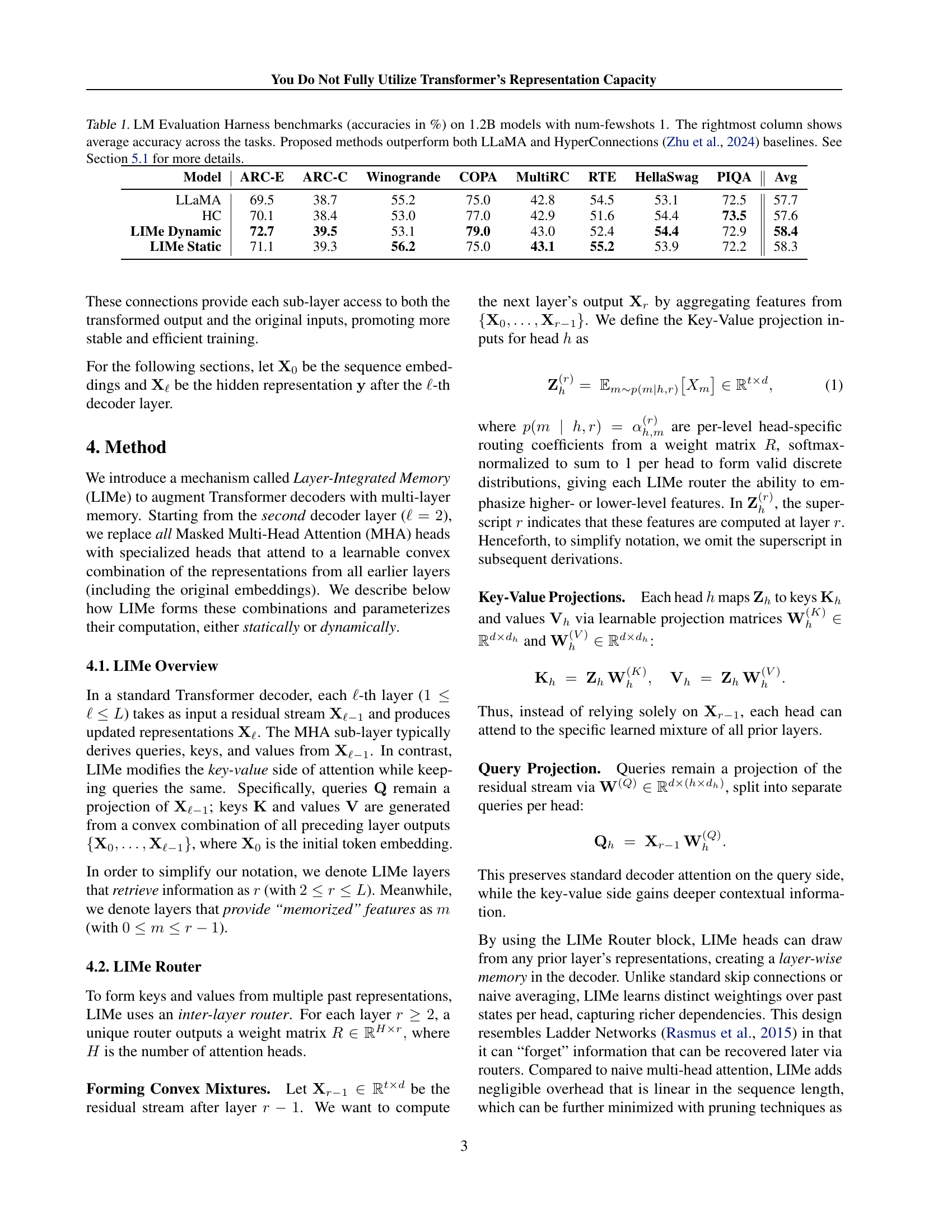
🔼 This figure displays the average weights assigned by each head in later layers (r) to representations from previous layers (m) in both the static and dynamic versions of the LIMe model. In the later layers of both models, there’s a greater tendency to retrieve information from earlier layers than from the immediately preceding layer. This is more pronounced in the dynamic LIMe model, where there’s a noticeable peak in the weight given to the very first layer.
read the caption
Figure 2: Mean retrieval weight for each representation (m𝑚mitalic_m) among later layers (r𝑟ritalic_r). In both cases, in the last layers, models tend to retrieve information from previous layers rather than from the current one. In the case of Dynamic LIMe, there is a clear bump in retrieving from the first layer. See Section 5.2 for more details.

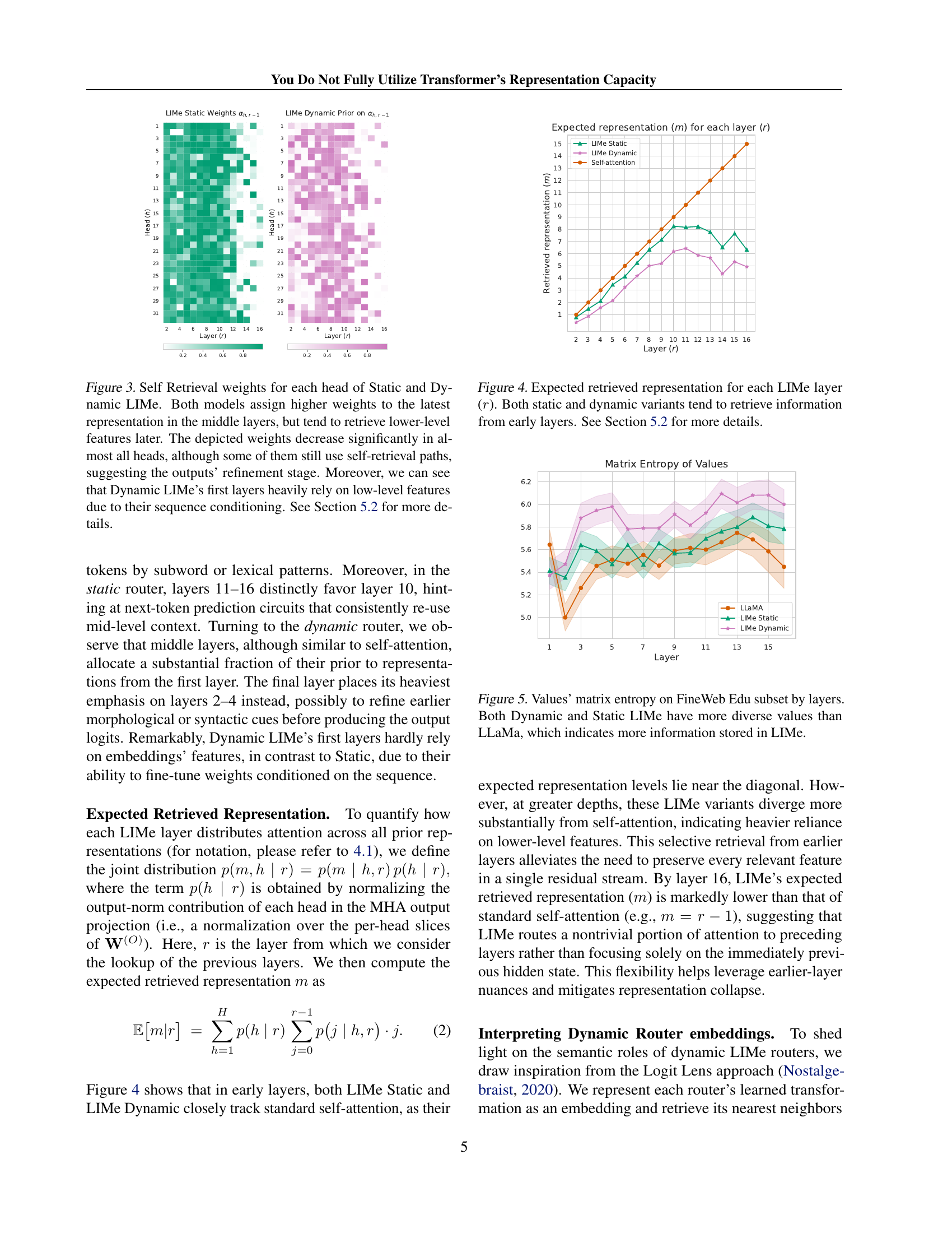
🔼 Figure 3 visualizes the self-retrieval weights for each attention head in both Static and Dynamic LIMe models across different layers. The heatmaps show the relative importance each head assigns to its own layer’s representation (self-retrieval) versus representations from earlier layers. In the middle layers, both models generally prioritize the immediately preceding layer’s output. However, as we move towards deeper layers, self-retrieval weight decreases for most heads, indicating that they increasingly incorporate information from earlier layers. This suggests a refinement process where earlier representations (low-level features) are re-introduced to refine the model’s output. Importantly, the figure highlights that Dynamic LIMe’s initial layers show a stronger reliance on earlier layer representations, likely due to sequence conditioning influencing how it prioritizes information.
read the caption
Figure 3: Self Retrieval weights for each head of Static and Dynamic LIMe. Both models assign higher weights to the latest representation in the middle layers, but tend to retrieve lower-level features later. The depicted weights decrease significantly in almost all heads, although some of them still use self-retrieval paths, suggesting the outputs’ refinement stage. Moreover, we can see that Dynamic LIMe’s first layers heavily rely on low-level features due to their sequence conditioning. See Section 5.2 for more details.

🔼 This figure visualizes the average weights assigned by each LIMe layer (r) to representations from previous layers (m). The x-axis represents the LIMe layer (r), and the y-axis shows the expected retrieved representation (m). It demonstrates that, regardless of whether a static or dynamic LIMe router is used, later LIMe layers tend to draw information more heavily from earlier layers than from the immediately preceding layer (m = r-1). This behavior suggests LIMe effectively integrates information from multiple layers, thereby mitigating representation collapse, a phenomenon where distinct features or tokens become indistinguishable in deeper layers.
read the caption
Figure 4: Expected retrieved representation for each LIMe layer (r𝑟ritalic_r). Both static and dynamic variants tend to retrieve information from early layers. See Section 5.2 for more details.

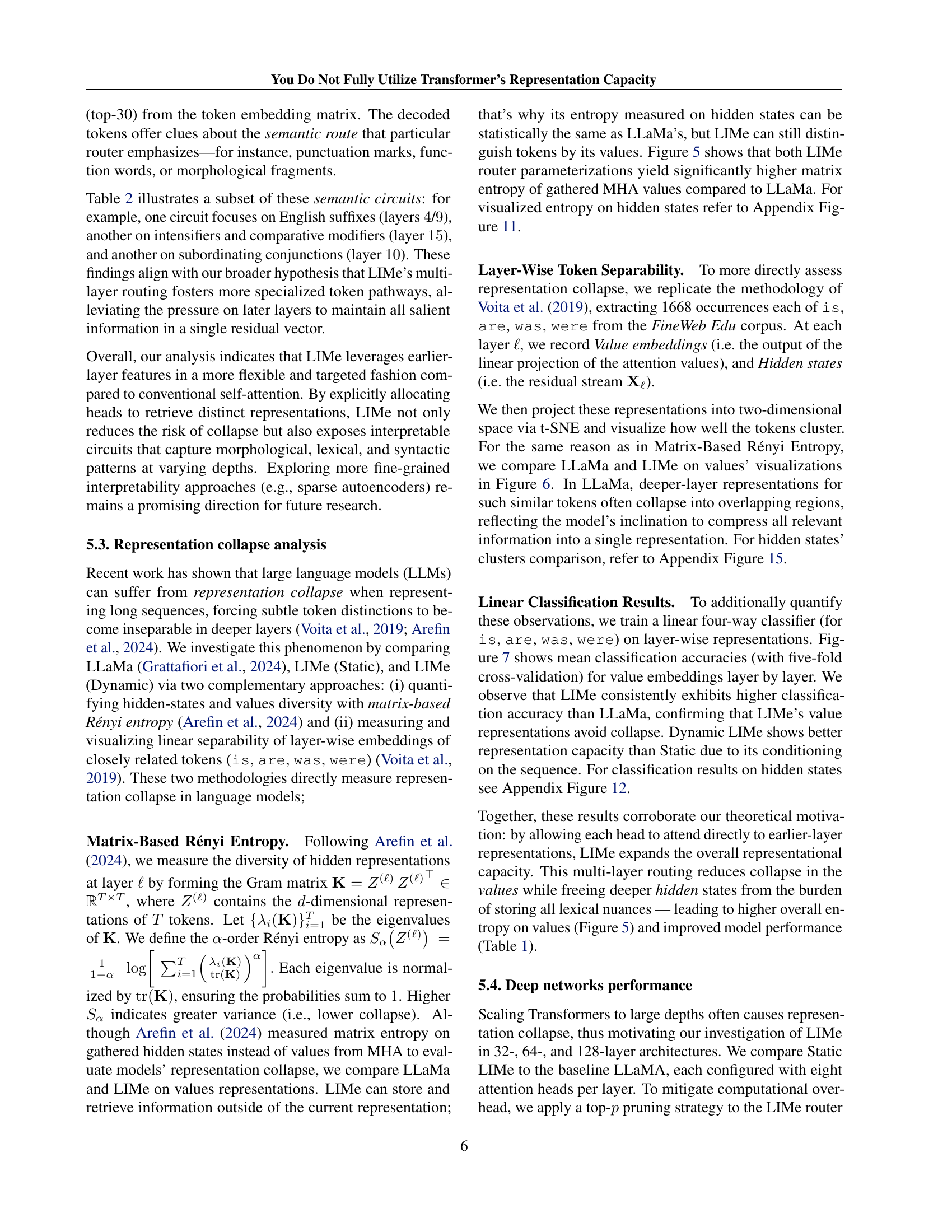
🔼 This figure displays the matrix entropy of the values (output of the value projection matrix in the multi-head self-attention mechanism) across different layers of three language models: LLaMa, LIMe Static, and LIMe Dynamic. Matrix entropy is a measure of the diversity of the values; higher entropy suggests a richer and more diverse representation. The plot shows how entropy changes across layers (x-axis) for each model. Both LIMe variants exhibit considerably higher entropy across all layers compared to LLaMa, indicating that LIMe models store and maintain significantly more information in their value representations than LLaMa.
read the caption
Figure 5: Values’ matrix entropy on FineWeb Edu subset by layers. Both Dynamic and Static LIMe have more diverse values than LLaMa, which indicates more information stored in LIMe.

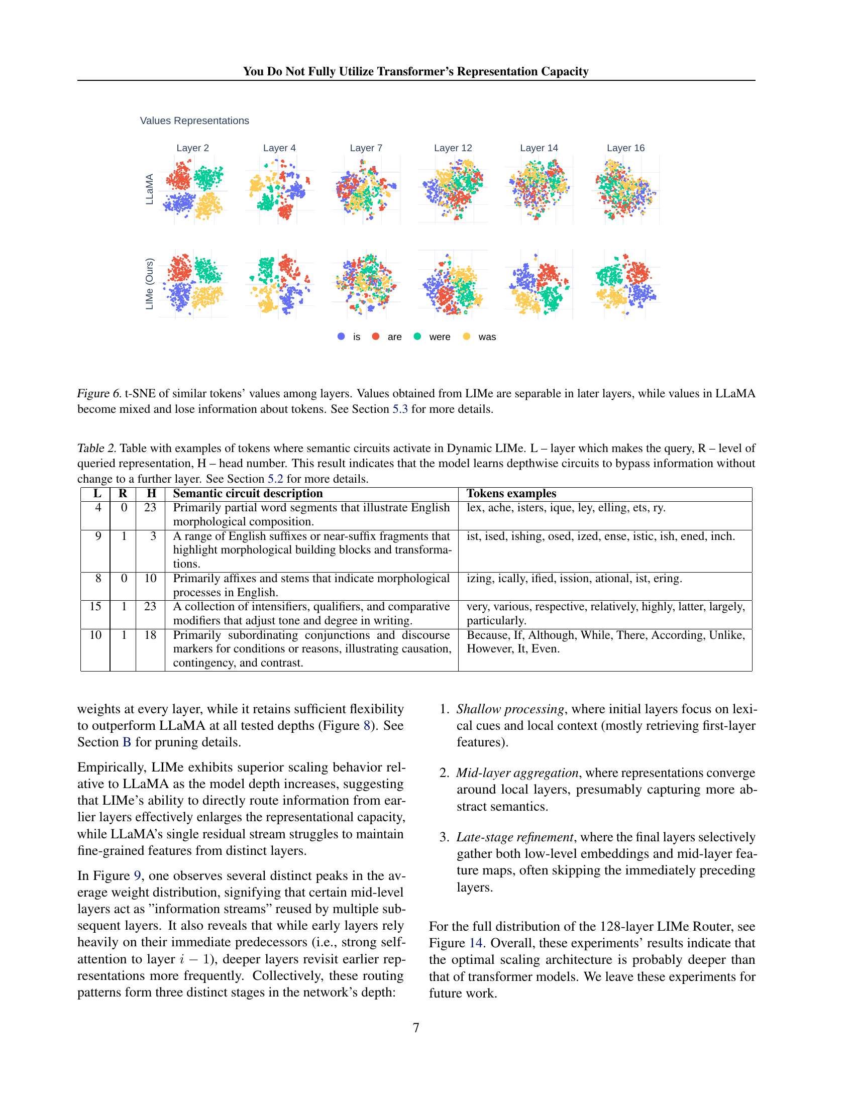
🔼 This figure visualizes the separation of similar tokens’ value representations across different layers in both LIMe and LLaMA models using t-SNE. In the LIMe model, the representations of similar tokens remain distinct even in deeper layers, indicating preservation of information. Conversely, in the LLaMA model, the representations of these similar tokens become increasingly mixed and less distinguishable in deeper layers, suggesting a loss of information as the model processes the sequence. This visualization supports the paper’s claim that LIMe is more effective at preventing representation collapse than LLaMA.
read the caption
Figure 6: t-SNE of similar tokens’ values among layers. Values obtained from LIMe are separable in later layers, while values in LLaMA become mixed and lose information about tokens. See Section 5.3 for more details.

🔼 This figure displays the accuracy of a linear classifier trained to distinguish between four closely related words (is, are, was, were) using their value representations from different layers of two language models: LIMe and LLaMA. The x-axis represents the layer number, and the y-axis shows the classification accuracy. LIMe consistently achieves near-perfect accuracy (approximately 1.0) in the deeper layers, indicating that its value representations effectively maintain the distinction between these words. In contrast, LLaMA’s accuracy is significantly lower, demonstrating that its representation of these words collapses in the deeper layers. This observation confirms that LIMe effectively prevents representation collapse, preserving the fine-grained differences between semantically similar tokens in deeper layers.
read the caption
Figure 7: Values classification accuracy measured with standard deviation over 5 cross-validation folds. Values in later layers obtained from LIMe can be linearly separated with nearly 1.0 accuracy, while accuracy for values from LLaMA is much lower. See Section 5.3 for more details.

🔼 This figure displays the training loss curves for models with varying depths (32, 64, and 128 layers). It compares the performance of the LIMe architecture against a baseline model. The results clearly show that LIMe achieves significantly lower training loss than the baseline, particularly for the deeper 128-layer model. This demonstrates LIMe’s ability to effectively handle the challenges of training very deep transformer networks.
read the caption
Figure 8: Training losses for deep architectures. The LIMe architecture significantly outperforms the baseline, especially in the case of 128128128128 layers. See Section 5.4 for more details.

🔼 Figure 9 analyzes the retrieval weights in a 128-layer LIMe model trained using top-p pruning. The green curve shows the average weight given to previous layers’ representations by each layer, revealing distinct peaks that suggest the model develops multiple, independent information streams in a self-supervised manner. The orange curve plots the average weight each layer assigns to its own immediately preceding layer’s representation (self-attention), which decreases as the network deepens. This decrease, coupled with the peaks in the green curve, indicates three distinct phases of information processing across the layers.
read the caption
Figure 9: Retrieval weights statistics for a 128-layer LIMe model trained with top-p𝑝pitalic_p pruning. The mean retrieval weight from subsequent layers (green curve) displays several distinct peaks, indicating that the model acquires multiple information streams in a self-supervised fashion. The mean self-retrieval weight (orange curve), where 1.0 denotes self-attention, decreases across later layers, forming three consecutive layer groups with different information-processing patterns. See Section 5.4 for further details.

🔼 This figure visualizes the average weights assigned by each LIMe layer to its own previous representation (self-retrieval) across all attention heads. It shows how much each layer relies on its immediate predecessor versus earlier layers. This helps illustrate how the LIMe mechanism balances the use of recent and past information in different layers of the transformer architecture, contrasting the behavior with standard self-attention.
read the caption
Figure 10: Self Retrieval weights averaged across heads for each LIMe layer.

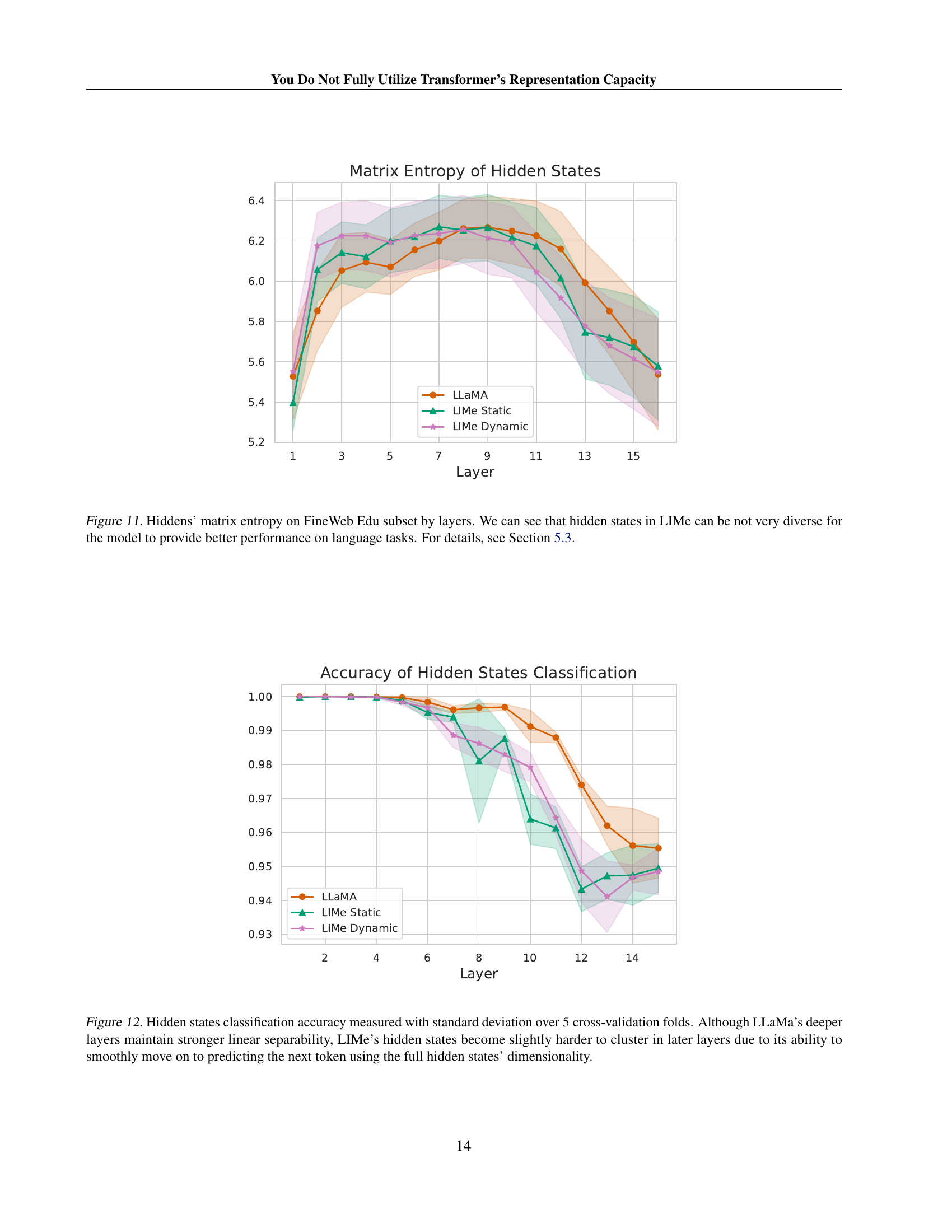
🔼 This figure displays the matrix entropy of hidden states across different layers of three language models: LLaMA, LIMe Static, and LIMe Dynamic, all trained on the FineWeb Edu dataset. Matrix entropy is a measure of the diversity of representations within a layer; higher entropy suggests more diverse and less collapsed representations. The plot shows that while LIMe models exhibit slightly lower entropy in some layers compared to LLaMA, this difference is not substantial, and LIMe still demonstrates significant performance gains. The relatively low entropy in later layers of all models may be due to the model compressing information into a smaller number of distinguishable representations, which is not directly correlated with model performance. For details, consult section 5.3 of the paper.
read the caption
Figure 11: Hiddens’ matrix entropy on FineWeb Edu subset by layers. We can see that hidden states in LIMe can be not very diverse for the model to provide better performance on language tasks. For details, see Section 5.3.

🔼 This figure displays the results of a linear classification experiment performed on hidden states of different language models. The models being compared are LLaMA, LIMe Static, and LIMe Dynamic. The x-axis represents the layer depth of the model, and the y-axis represents the accuracy of a classifier trained to distinguish between four closely related tokens (‘is’, ‘are’, ‘was’, ‘were’). LLaMa shows higher accuracy in later layers due to stronger linear separability of its hidden states. However, LIMe, particularly the dynamic version, shows a decrease in accuracy in deeper layers. This is attributed to LIMe’s ability to effectively use the full dimensionality of its hidden states for next-token prediction, which makes the states slightly harder to classify linearly.
read the caption
Figure 12: Hidden states classification accuracy measured with standard deviation over 5 cross-validation folds. Although LLaMa’s deeper layers maintain stronger linear separability, LIMe’s hidden states become slightly harder to cluster in later layers due to its ability to smoothly move on to predicting the next token using the full hidden states’ dimensionality.

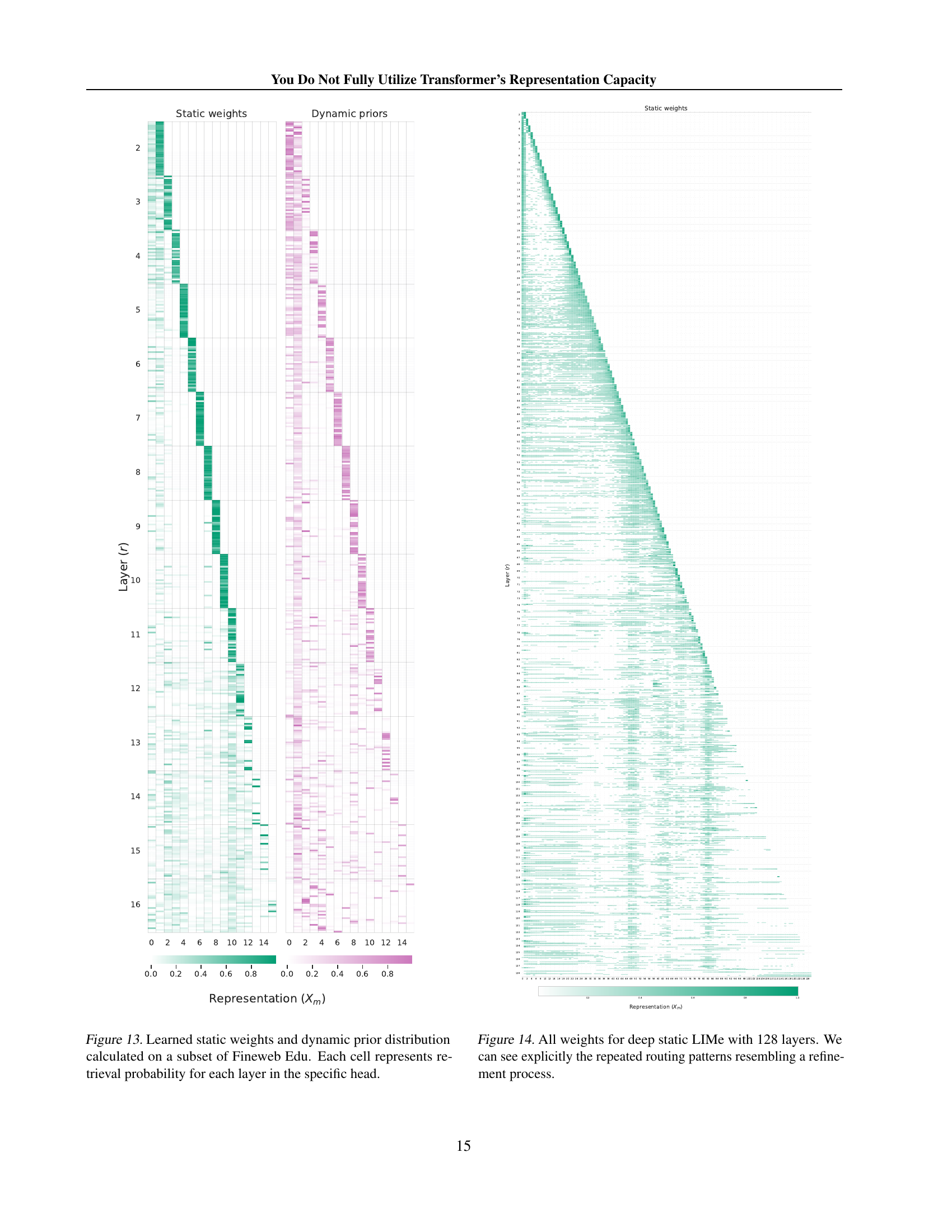
🔼 This figure visualizes the learned weights of both static and dynamic LIMe routers. The heatmaps show the probability with which each attention head in a given layer attends to the representations from previous layers. The x-axis represents the previous layer (0 being the embedding layer), and the y-axis represents the layer currently being processed. Each cell’s color intensity indicates the attention weight for a specific head and source layer combination. The left shows the static weights (one set of weights per head across all examples), while the right shows dynamic weights (weights computed per token). The visualization allows analysis of how the models integrate information from multiple layers during the processing of a sequence, specifically highlighting differences between static and dynamic routing schemes.
read the caption
Figure 13: Learned static weights and dynamic prior distribution calculated on a subset of Fineweb Edu. Each cell represents retrieval probability for each layer in the specific head.
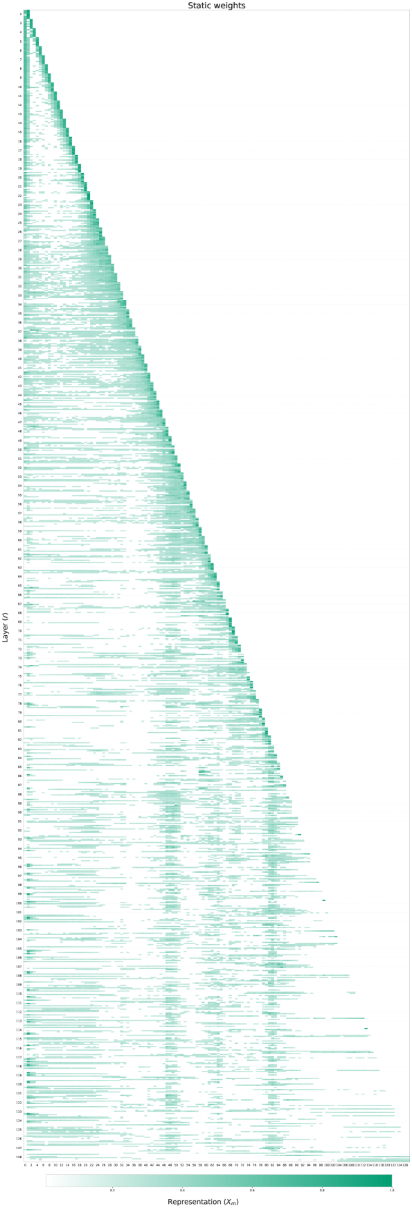
🔼 This figure visualizes the learned weights of the static LIMe router across all 128 layers of a deep transformer model. Each cell’s color intensity represents the weight assigned to a specific previous layer’s representation when computing the keys and values for the current layer’s self-attention mechanism. The pattern reveals a hierarchical information flow, with repeated, distinct routing patterns suggesting a multi-stage refinement process where information is iteratively processed and combined from various previous layers, rather than solely relying on the immediately preceding layer.
read the caption
Figure 14: All weights for deep static LIMe with 128 layers. We can see explicitly the repeated routing patterns resembling a refinement process.

🔼 This figure uses t-SNE to visualize the hidden states of similar tokens (is, are, was, were) across different layers of LLAMA and LIMe. While both models show some mixing of these tokens in deeper layers, LIMe demonstrates better separation of these tokens in later layers than LLAMA. This is because, unlike LLAMA, LIMe updates hidden states by also attending to previous representations, mitigating the information loss and collapse that occurs in standard transformers. This improvement in separability is consistent with the reduced representation collapse shown by LIMe in section 5.3.
read the caption
Figure 15: t-SNE of similar tokens’ hidden states among layers. Although hidden states are not separable in later layers for both models, unlike LLaMA, LIMe can make updates attending to the previous representations, which leads to high values’ separability. See Section 5.3 for more details.
More on tables
| L | R | H | Semantic circuit description | Tokens examples |
|---|---|---|---|---|
| 4 | 0 | 23 | Primarily partial word segments that illustrate English morphological composition. | lex, ache, isters, ique, ley, elling, ets, ry. |
| 9 | 1 | 3 | A range of English suffixes or near-suffix fragments that highlight morphological building blocks and transformations. | ist, ised, ishing, osed, ized, ense, istic, ish, ened, inch. |
| 8 | 0 | 10 | Primarily affixes and stems that indicate morphological processes in English. | izing, ically, ified, ission, ational, ist, ering. |
| 15 | 1 | 23 | A collection of intensifiers, qualifiers, and comparative modifiers that adjust tone and degree in writing. | very, various, respective, relatively, highly, latter, largely, particularly. |
| 10 | 1 | 18 | Primarily subordinating conjunctions and discourse markers for conditions or reasons, illustrating causation, contingency, and contrast. | Because, If, Although, While, There, According, Unlike, However, It, Even. |
🔼 This table presents examples illustrating how Dynamic LIMe learns depthwise circuits. Each row shows a token, the layer (L) generating the query, the level of representation (R) from which the information is drawn, the head (H) used, and a description of the identified semantic circuit. The examples demonstrate that the model selectively accesses earlier layer representations to process specific linguistic features (like suffixes or subordinating conjunctions) without modifying the information before passing it to subsequent layers.
read the caption
Table 2: Table with examples of tokens where semantic circuits activate in Dynamic LIMe. L – layer which makes the query, R – level of queried representation, H – head number. This result indicates that the model learns depthwise circuits to bypass information without change to a further layer. See Section 5.2 for more details.
| Hyperparameter | Value |
|---|---|
| Optimizer | AdamW |
| Learning Rate | 0.001 |
| LIMe Router Learning Rate | 0.01 |
| Weight Decay | 0.1 |
| 0.9 | |
| 0.95 | |
| Scheduler | cosine |
| Warmup Steps | 200 |
| Min LR | |
| Mixed Precision | bf16 |
| Gradient Clipping | 1.0 |
| Sequence Length | 2048 |
| Batch Size | 1024 |
| Training Steps | 20,000 |
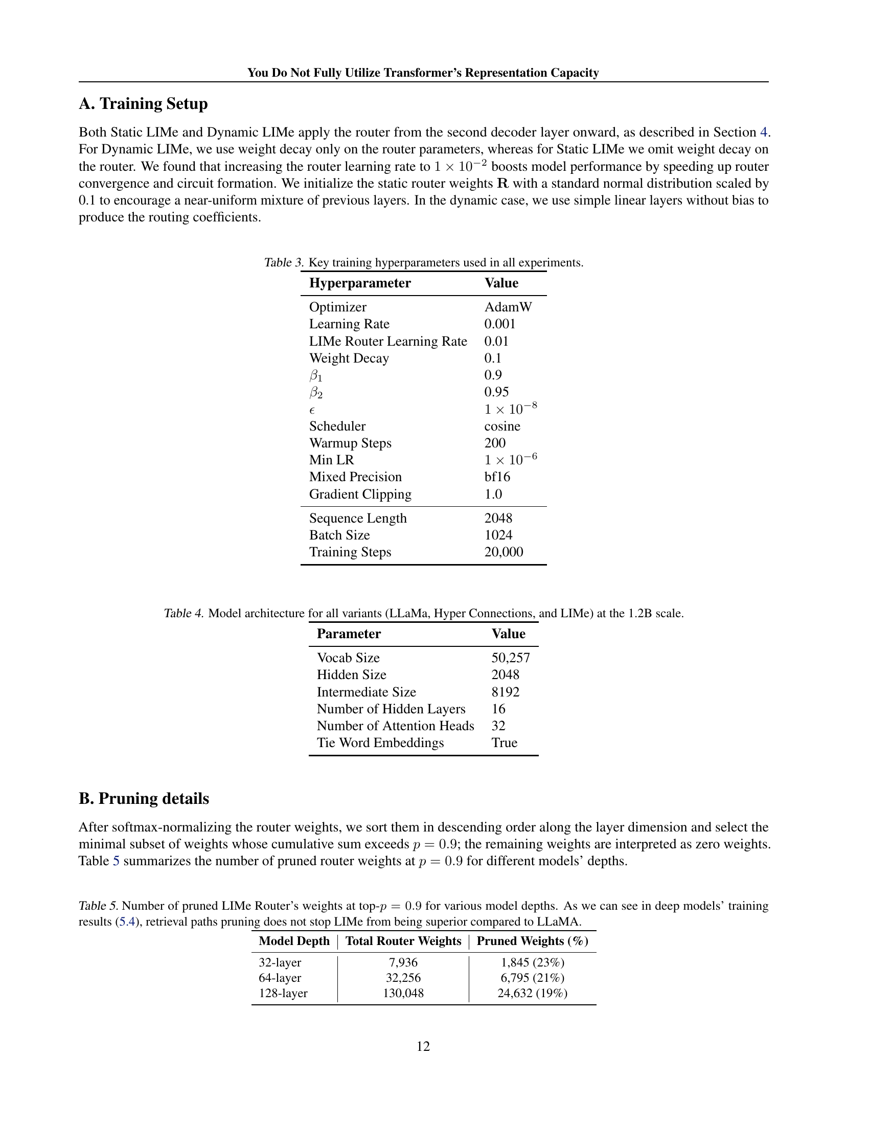
🔼 This table lists the key hyperparameters used during the training process of all the models presented in the paper. It includes details such as the optimizer used (AdamW), the learning rate for the main model and the specialized LIMe router, weight decay, beta parameters for AdamW, the learning rate scheduler used (cosine), the number of warmup steps, the minimum learning rate, the mixed precision setting used (bf16), the gradient clipping value, the sequence length used during training, the batch size, and the total number of training steps.
read the caption
Table 3: Key training hyperparameters used in all experiments.
| Parameter | Value |
| Vocab Size | 50,257 |
| Hidden Size | 2048 |
| Intermediate Size | 8192 |
| Number of Hidden Layers | 16 |
| Number of Attention Heads | 32 |
| Tie Word Embeddings | True |
🔼 This table details the architecture of the language models used in the experiments: LLaMa, Hyper Connections, and LIMe. It provides a comparison of key architectural parameters for all three models, all scaled to 1.2 billion parameters. This allows for a direct comparison of their performance in the context of the paper’s experiments.
read the caption
Table 4: Model architecture for all variants (LLaMa, Hyper Connections, and LIMe) at the 1.2B scale.
| Model Depth | Total Router Weights | Pruned Weights (%) |
|---|---|---|
| 32-layer | 7,936 | 1,845 (23%) |
| 64-layer | 32,256 | 6,795 (21%) |
| 128-layer | 130,048 | 24,632 (19%) |
🔼 This table shows the number of pruned LIMe Router weights for different model depths when using a top-p pruning strategy of 0.9. The top-p pruning method sets weights below a certain threshold to zero, effectively reducing computational cost. Importantly, even with this aggressive pruning, the results in section 5.4 demonstrate that LIMe still outperforms LLaMA in terms of performance.
read the caption
Table 5: Number of pruned LIMe Router’s weights at top-p=0.9𝑝0.9p=0.9italic_p = 0.9 for various model depths. As we can see in deep models’ training results (5.4), retrieval paths pruning does not stop LIMe from being superior compared to LLaMA.
| Model | # Parameters (B) | FLOPs (T) | Peak Memory Overhead over LLaMA excluding parameters | |
|---|---|---|---|---|
| Train | Inference | |||
| LLaMA | 0 | 0 | ||
| LIMe Static | (+0.008%) | (+0.3%) | ||
| LIMe Dynamic | (+0.075%) | (+1.3%) | ||
| HC Dynamic | (+0.030%) | (+0.3%) | ||
🔼 Table 6 compares the efficiency of various 1.2B parameter models: the baseline LLaMA model, the proposed LIMe models (both static and dynamic versions), and the Hyper-Connections (HC) model. The comparison focuses on the number of parameters, FLOPs (floating-point operations), peak memory usage during training, and peak memory usage during inference. The table highlights that LIMe models have negligible increases in parameters and FLOPs compared to LLaMA, while also showing significantly lower peak memory usage during both training and inference (especially when a key-value cache is used). Acronyms used are defined: H (number of heads), L (number of layers), T (sequence length), D (hidden dimension), R (Hyper Connections expansion rate).
read the caption
Table 6: Comparing efficiency for all 1.21.21.21.2B models: both Dynamic and Static LIMe enjoy negligible parameter and FLOPs increase, and smaller peak memory than HC during training. When the Key-Value cache is utilized, this memory advantage extends to inference as well (*). H – number of heads, L — number of layers, T — sequence length, D — hidden dimension, R — Hyper Connections (Zhu et al., 2024) expansion rate.
Full paper#