MUDDFormer: Breaking Residual Bottlenecks in Transformers via Multiway Dynamic Dense Connections

2502.12170

Da Xiao et el.

🤗 2025-02-19

TL;DR
#

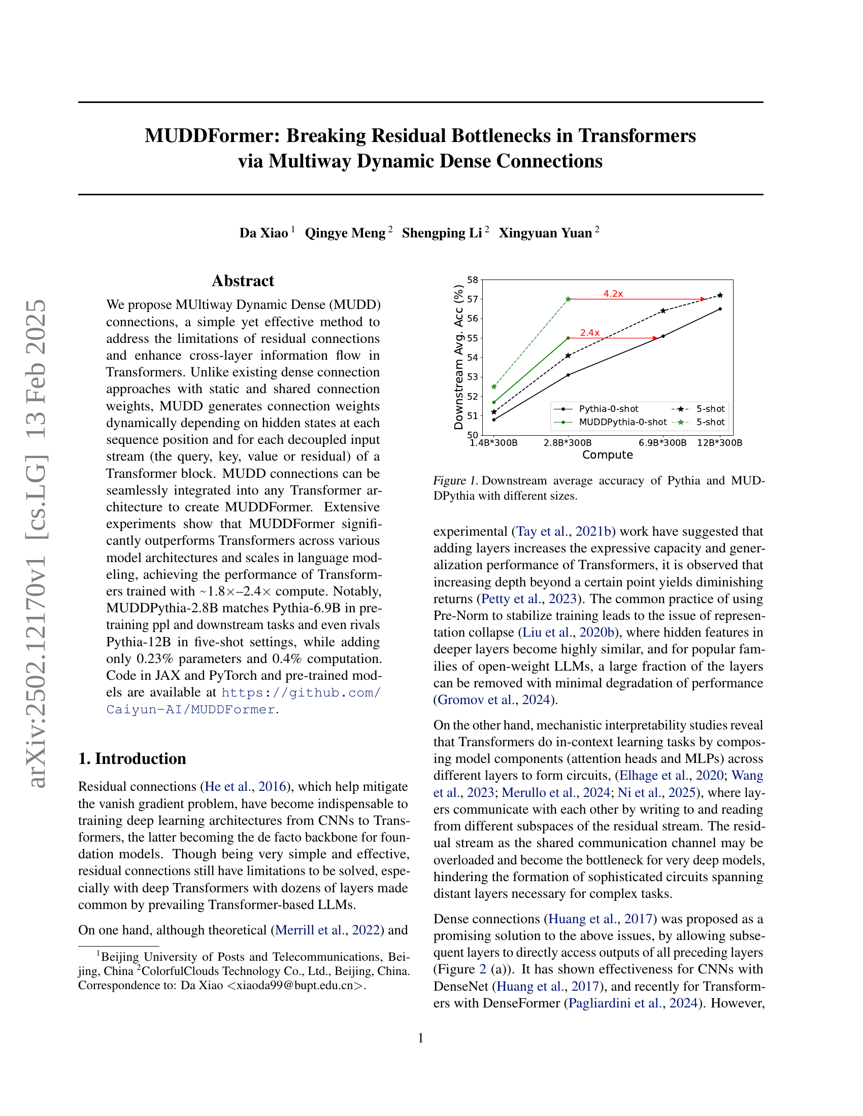
Large Language Models (LLMs) based on Transformers often suffer from limitations in information flow between layers, hindering performance and scalability. This is particularly pronounced in deep models where the residual connections, a standard component, struggle to efficiently transmit information across numerous layers, leading to performance plateaus and computational bottlenecks.

The proposed MUDDFormer tackles this problem by introducing ‘Multiway Dynamic Dense (MUDD) connections’. These connections dynamically adjust their weights based on the model’s internal states at each layer, thereby significantly enhancing information flow. Experimental results demonstrate that MUDDFormer substantially outperforms standard Transformers across various model sizes and downstream tasks, often matching or even exceeding the performance of much larger models while requiring significantly less compute. This improvement is attributed to the enhanced cross-layer communication facilitated by MUDD connections. The method’s seamless integrability with existing architectures also makes it highly adaptable and promising for future LLM development.

Key Takeaways
#

Why does it matter?
#

This paper is crucial because it introduces MUDD connections, a novel approach to enhance information flow in Transformers. This addresses a critical limitation of existing Transformer architectures, paving the way for more efficient and powerful large language models. It offers significant performance improvements with minimal added computational cost, opening new avenues for research in model scaling and architectural design.

Visual Insights
#

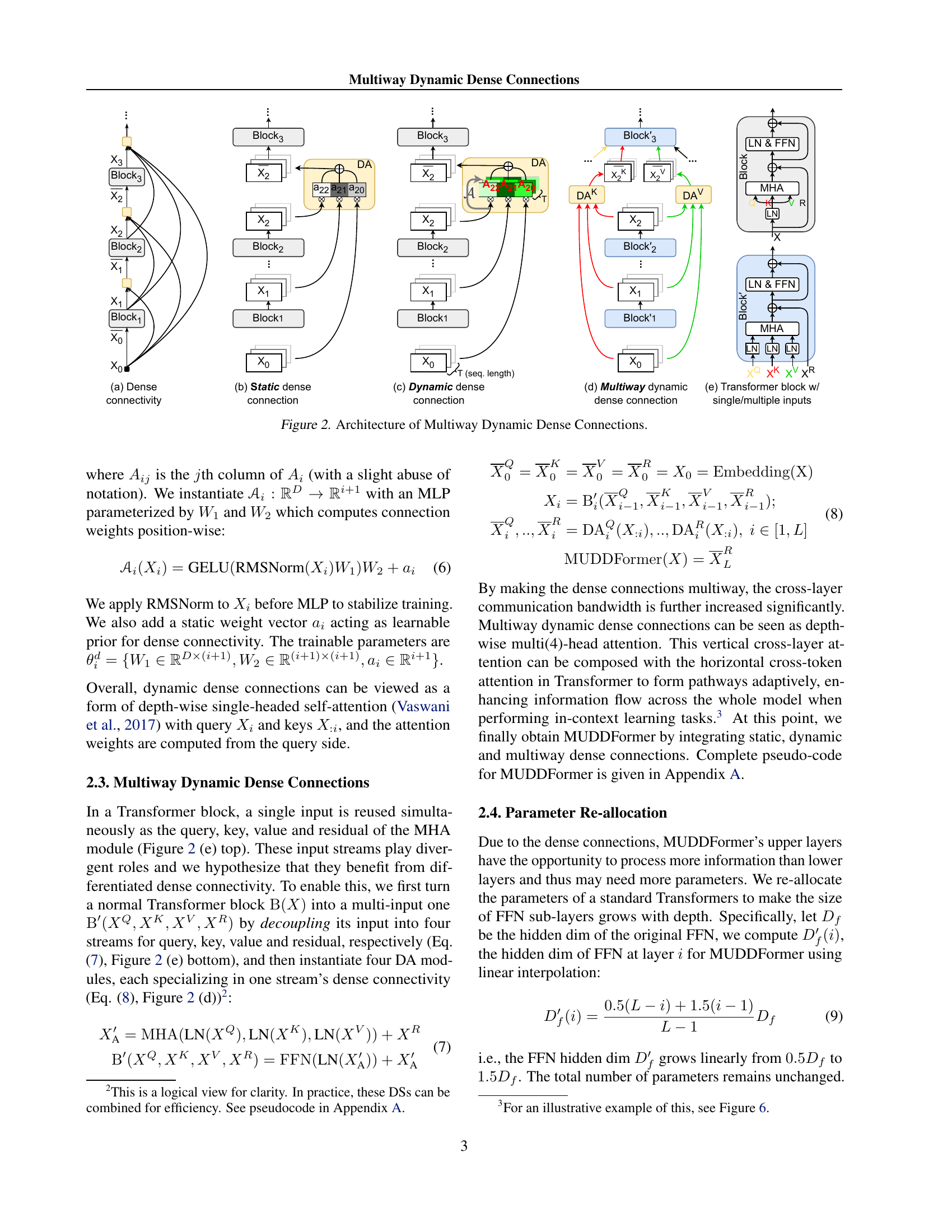
Model Size	$\mathrm{R_{\Delta params}}$	$\mathrm{R_{\Delta FLOPs}}$	L	D	T	$\mathrm{\eta}=$ $\mathrm{\frac{L+3}{D}}$	$\mathrm{\rho}=$ $\mathrm{\frac{T}{D}}$
1.4B	$0.22\%$	$0.38\%$	24	2048	4096	0.0132	2
1.34B	$0.49\%$	$0.8\%$	42	1536	4096	0.0293	2.67
2.8B	$0.23\%$	$0.4\%$	32	2560	4096	0.0137	1.6
6.9B	$0.14\%$	$0.26\%$	32	4096	4096	0.0085	1
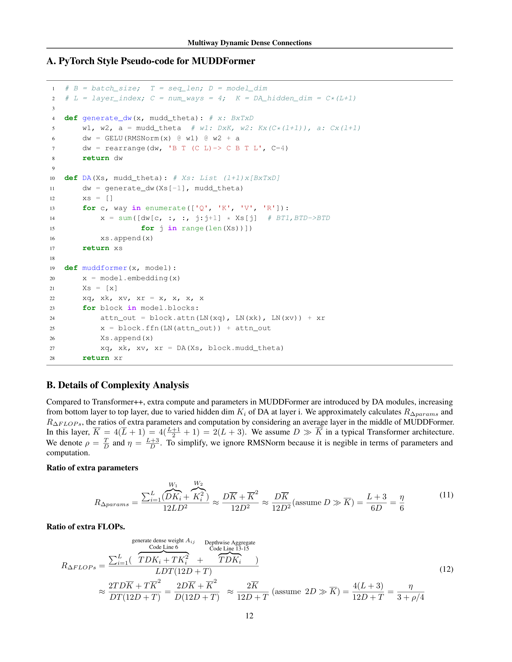
Formula	$\displaystyle{\frac{\eta}{6}}$	$\displaystyle{\frac{\eta}{3+\rho/4}}$

🔼 This table presents the additional computational cost and parameter overhead introduced by the MUDD connections. It compares analytical results with concrete examples. The analytical portion provides formulas showing the relationship between the extra parameters and computation to the total model size, depth (number of layers, L), and sequence length (T). The concrete examples use typical values for these parameters to demonstrate the relative overhead.
read the caption
Table 1: Ratios of extra parameters and computation introduced by MUDD connections: (last row) analytical results and (upper rows) concrete values for typical model architectures and hyperparameters. L = number of layers, T = sequence length.

In-depth insights
#

Residual Bottleneck
#

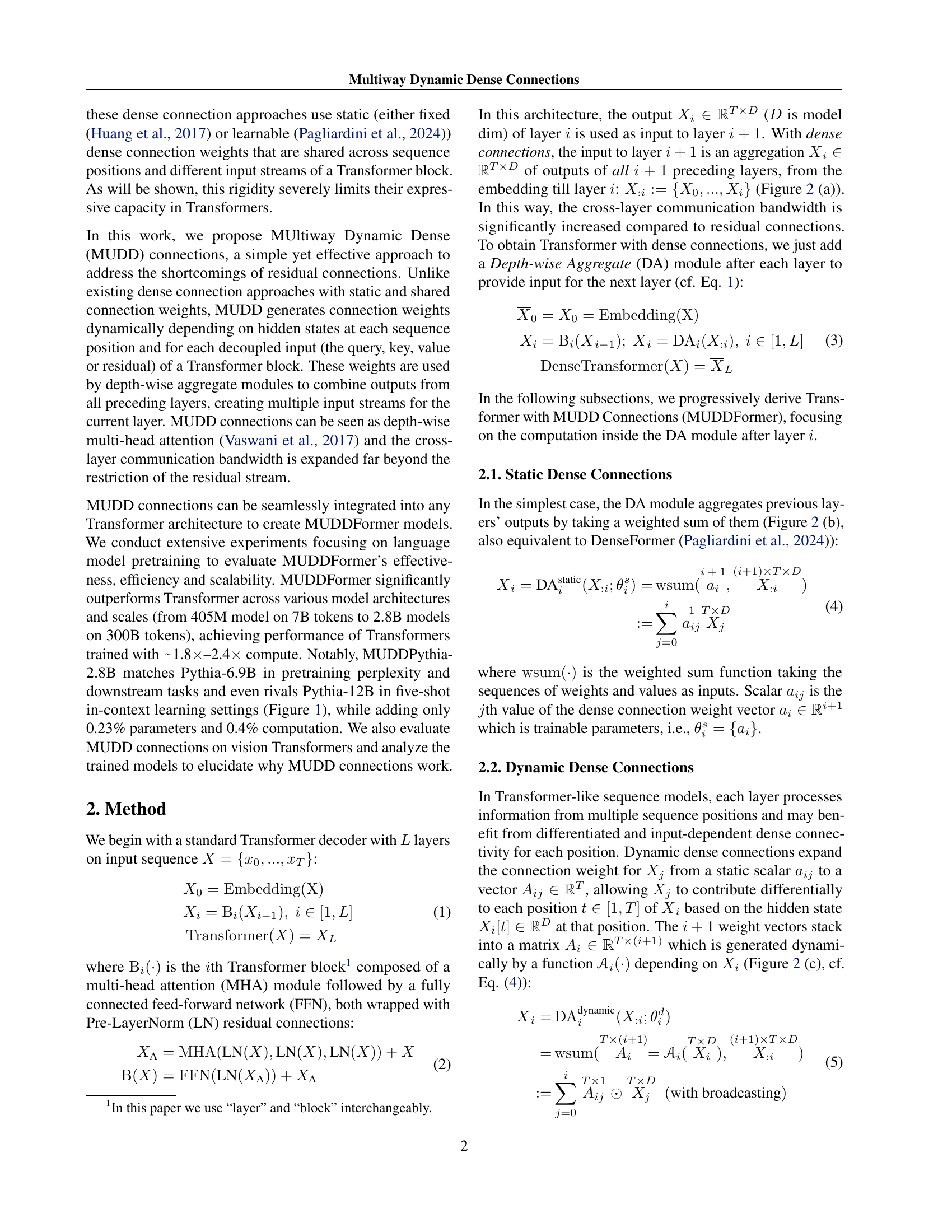
The concept of a “Residual Bottleneck” in deep learning, particularly within Transformers, highlights the limitations of residual connections in handling information flow as network depth increases. Standard residual connections, while effective in mitigating vanishing gradients in shallower networks, become inadequate in deeper architectures. The residual stream, acting as a shared communication channel, can become overloaded, hindering effective cross-layer information exchange crucial for complex tasks. This bottleneck limits the formation of sophisticated circuits spanning multiple layers, thereby restricting the model’s ability to learn and generalize effectively. The paper addresses this by proposing Multiway Dynamic Dense (MUDD) connections, a mechanism designed to enhance cross-layer information flow and overcome this bottleneck. MUDD generates dynamic connection weights, tailored to each sequence position and input stream, allowing for flexible and adaptive communication between layers, thus breaking the residual bottleneck and improving performance.

MUDD Connections
#

The core concept of “MUDD Connections” revolves around enhancing information flow within Transformer networks by dynamically generating connection weights, unlike traditional static approaches. Multiway connections are key, processing queries, keys, values, and residuals independently to avoid bottlenecks in the residual stream. The dynamic aspect is crucial as weights adapt based on hidden states at each position, allowing the model to learn intricate relationships. This dynamic multiway approach enhances expressiveness and facilitates cross-layer information flow beyond the limitations of residual connections, resulting in improved performance. The implementation seamlessly integrates into existing Transformer architectures, forming the foundation of the MUDDFormer model. Efficiency is also a focus, with minimal parameter and computational overhead. The effectiveness of MUDD Connections is validated through experiments showing substantial performance gains compared to baselines in language and vision tasks. This innovative approach is a significant step towards creating more sophisticated and efficient Transformer models.

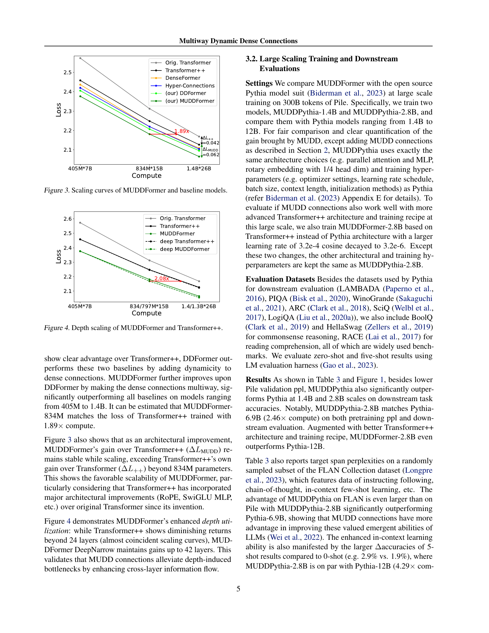
Scaling Experiments
#

The scaling experiments section of a research paper is crucial for evaluating the performance and efficiency of a novel model, especially in deep learning. It investigates how the model behaves as key parameters, such as model size (number of parameters), dataset size, and computational resources, are varied. A well-designed scaling experiment should demonstrate the model’s ability to generalize and scale gracefully, revealing potential limitations or bottlenecks. Key insights from such experiments often include performance gains relative to existing models, computational efficiency, and the establishment of scaling laws. The experiments might use different model architectures, training methods, or datasets to thoroughly analyze the model’s scaling behavior. The presentation of results typically involves plots and tables that visually illustrate the relationships between model parameters and performance metrics. Analysis of these results helps to understand the model’s strengths, limitations, and overall scalability. Furthermore, the paper should also explore if the scaling behavior matches theoretical predictions or existing scaling laws, contributing to a comprehensive understanding of the model’s capabilities.

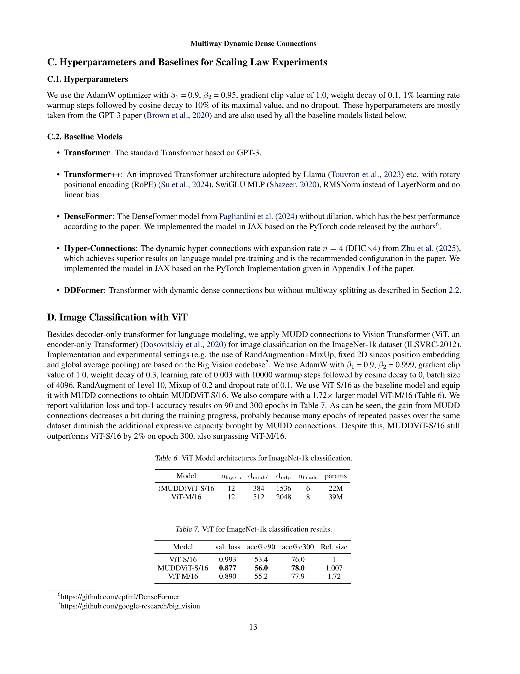
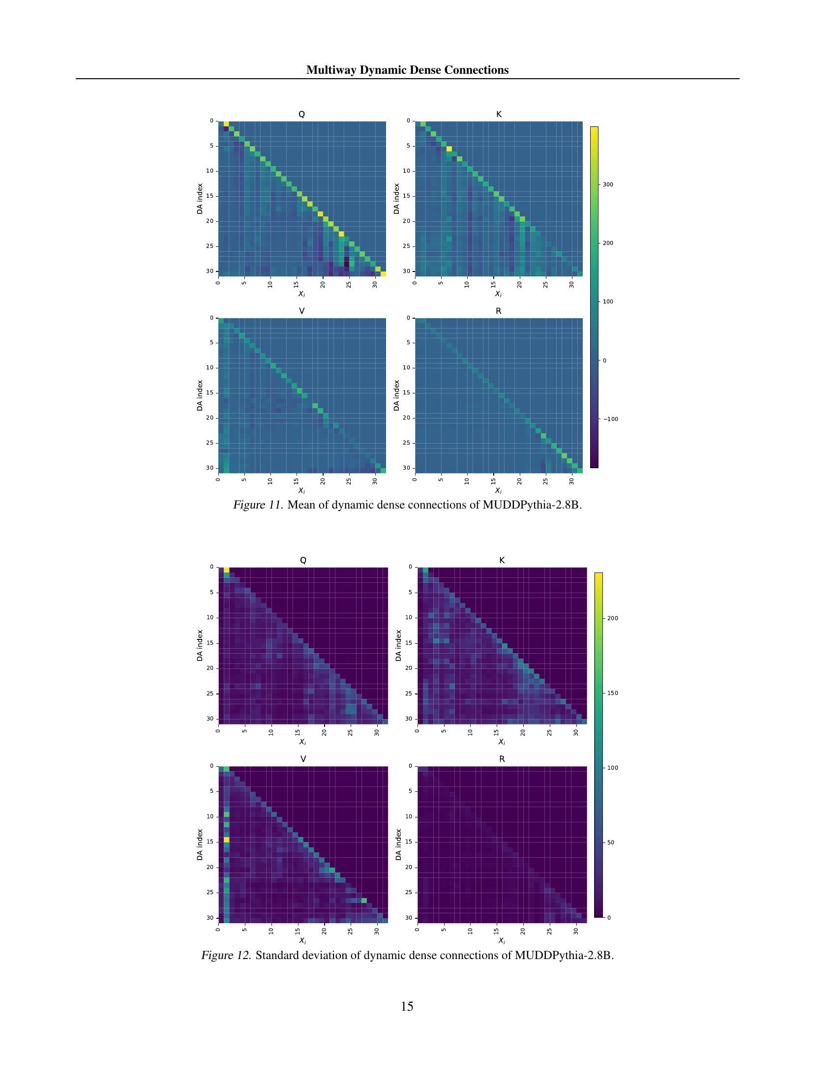
Mechanism Analysis
#

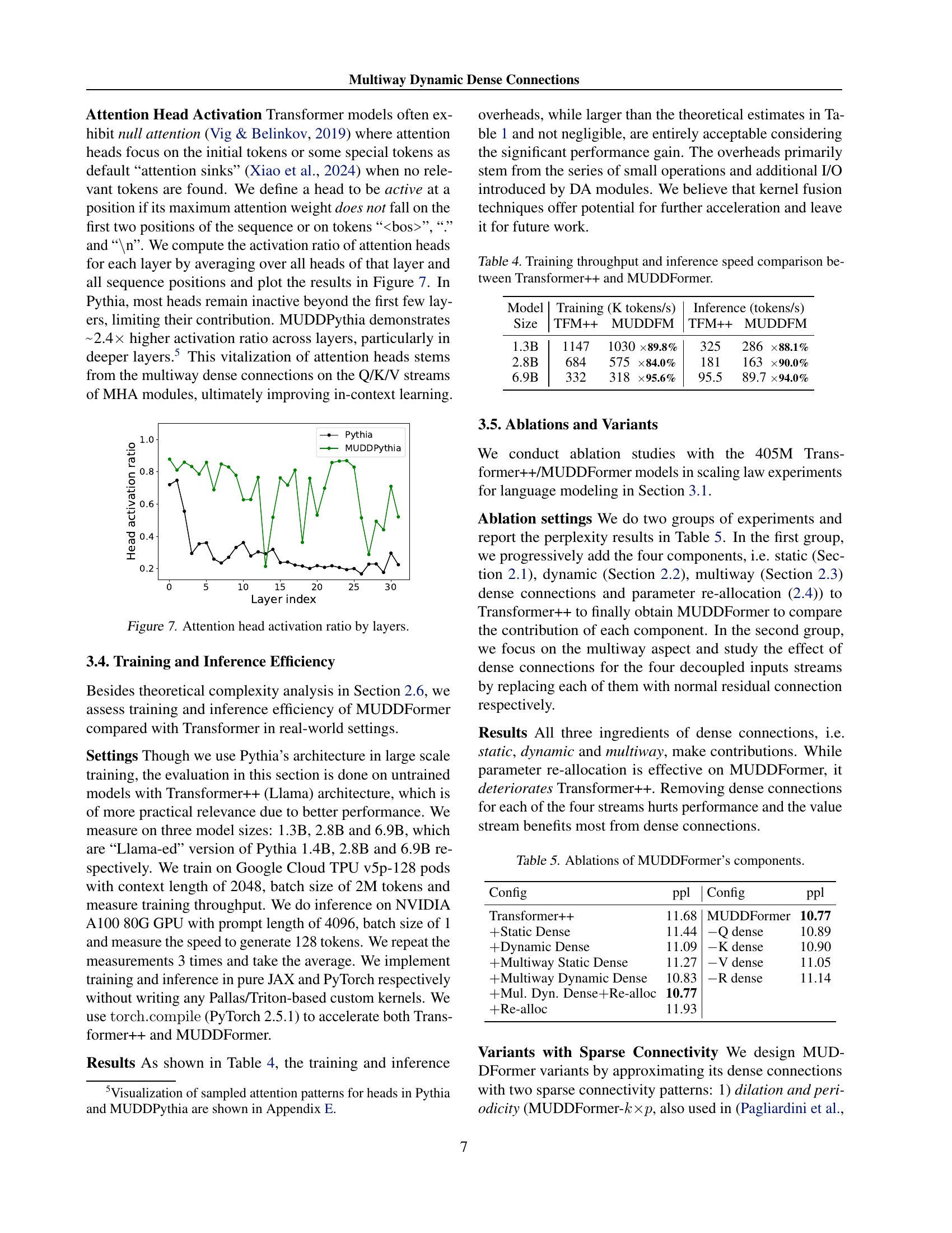
A mechanistic analysis of the model would involve investigating the internal workings and information flow to understand why it achieves superior performance. This could involve analyzing attention head activation patterns, identifying key pathways of information flow between layers, and examining how the model processes information from multiple sequence positions and input streams. Visualizing dynamic dense connection weights across layers could reveal insights into how cross-layer communication enhances performance. By comparing these patterns in the improved model versus a standard Transformer, researchers could pinpoint the specific mechanisms contributing to the observed benefits. Investigating representation collapse would also be crucial. A comparison of the cosine similarity between layers could show whether the model alleviates representation collapse and maintains information diversity. Furthermore, analyzing attention head activity in the various layers could highlight whether the model enhances attention mechanisms and reduces inactivity, leading to more effective in-context learning. This multi-faceted analysis would reveal precisely how the architectural innovations translate into concrete performance improvements.

Future Work
#

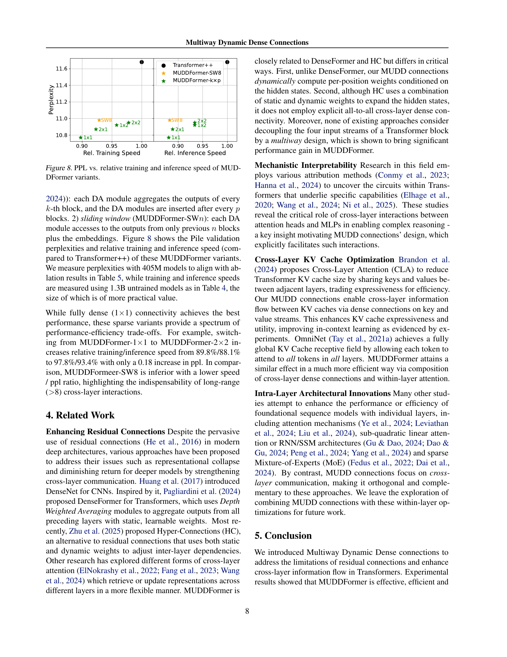
Future research directions stemming from this work on MUDDFormer could explore several promising avenues. Extending MUDD connections to other transformer architectures beyond decoders and encoders would be beneficial, potentially including sequence-to-sequence models. Investigating the interplay of MUDD with other architectural innovations such as different attention mechanisms or sparse attention is key. The impact of MUDD on various downstream tasks beyond language modeling warrants further exploration. A thorough analysis of the computational cost of MUDD, specifically methods for optimization, will improve efficiency. Finally, research into the theoretical underpinnings of MUDD’s success will provide a deeper understanding of its effectiveness.

More visual insights
#

More on tables

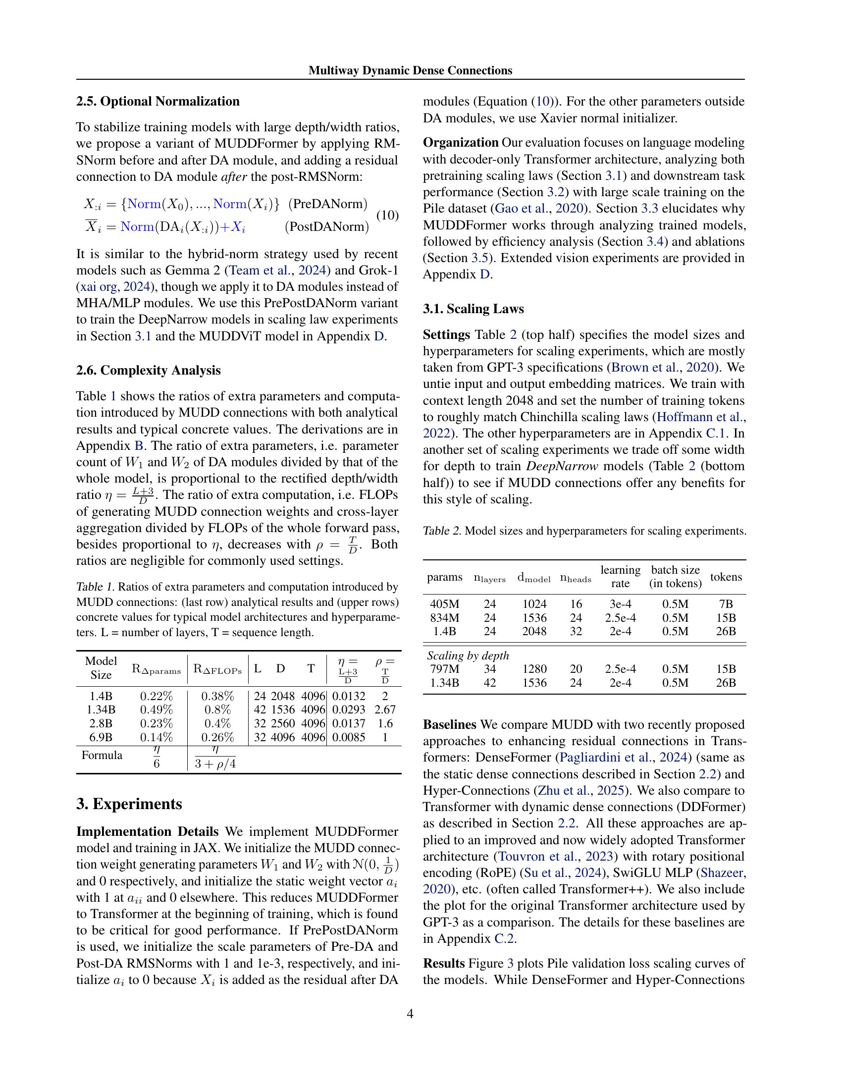
params	$\mathrm{n_{layers}}$	$\mathrm{d_{model}}$	$\mathrm{n_{heads}}$	learning rate	batch size (in tokens)	tokens
405M	24	1024	16	3e-4	0.5M	7B
834M	24	1536	24	2.5e-4	0.5M	15B
1.4B	24	2048	32	2e-4	0.5M	26B
Scaling by depth
797M	34	1280	20	2.5e-4	0.5M	15B
1.34B	42	1536	24	2e-4	0.5M	26B

🔼 This table presents the configurations of different model sizes used in the scaling experiments. It details the number of parameters, layers, model dimension (d_model), number of attention heads, learning rate, batch size (in tokens), and total number of training tokens for each model variant. The table is divided into two parts: one for scaling by depth and another for DeepNarrow models, where the scaling approach is different. The hyperparameters are primarily taken from the GPT-3 specifications (Brown et al., 2020) with adjustments made to align with Chinchilla scaling laws (Hoffmann et al., 2022).
read the caption
Table 2: Model sizes and hyperparameters for scaling experiments.

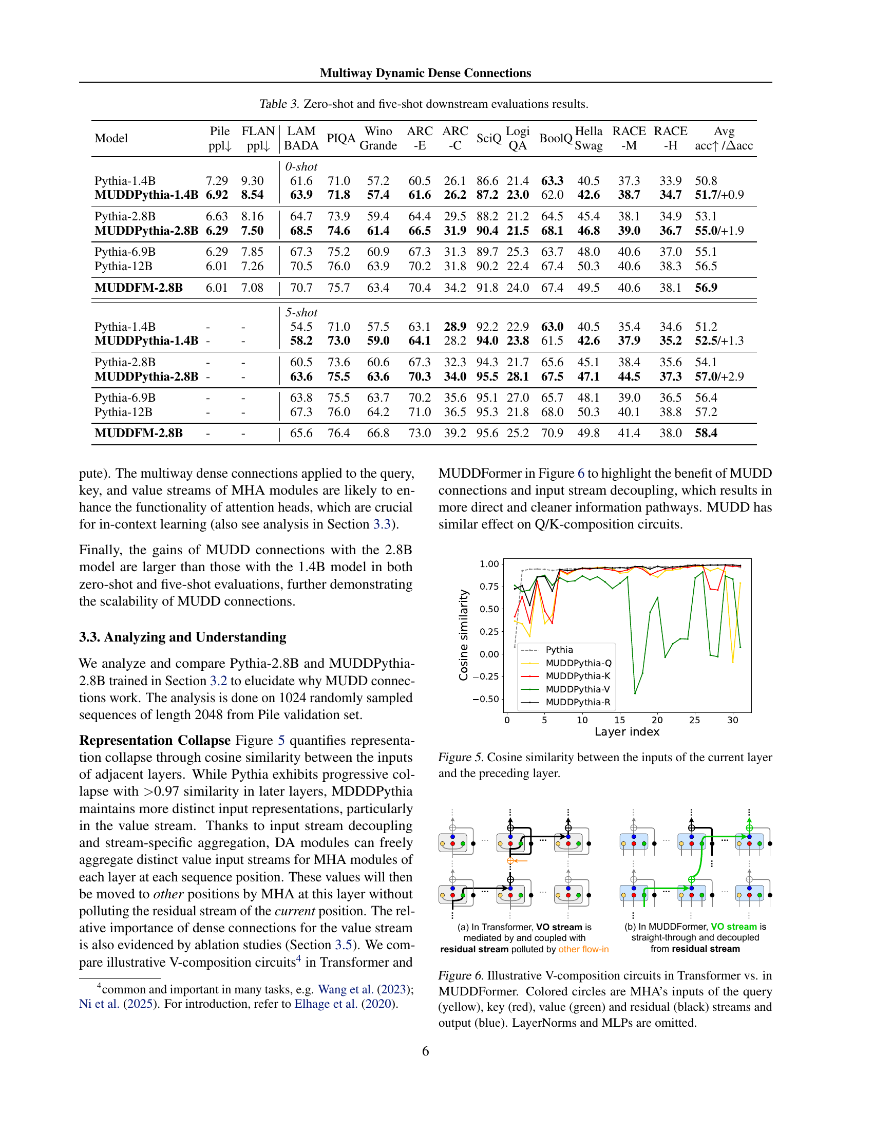
Model	Pile ppl $\downarrow$	FLAN ppl $\downarrow$	LAM BADA	PIQA	Wino Grande	ARC -E	ARC -C	SciQ	Logi QA	BoolQ	Hella Swag	RACE -M	RACE -H	Avg acc $\uparrow$ / $\Delta$ acc
			0-shot
Pythia-1.4B	7.29	9.30	61.6	71.0	57.2	60.5	26.1	86.6	21.4	63.3	40.5	37.3	33.9	50.8
MUDDPythia-1.4B	6.92	8.54	63.9	71.8	57.4	61.6	26.2	87.2	23.0	62.0	42.6	38.7	34.7	51.7/+0.9
Pythia-2.8B	6.63	8.16	64.7	73.9	59.4	64.4	29.5	88.2	21.2	64.5	45.4	38.1	34.9	53.1
MUDDPythia-2.8B	6.29	7.50	68.5	74.6	61.4	66.5	31.9	90.4	21.5	68.1	46.8	39.0	36.7	55.0/+1.9
Pythia-6.9B	6.29	7.85	67.3	75.2	60.9	67.3	31.3	89.7	25.3	63.7	48.0	40.6	37.0	55.1
Pythia-12B	6.01	7.26	70.5	76.0	63.9	70.2	31.8	90.2	22.4	67.4	50.3	40.6	38.3	56.5
MUDDFM-2.8B	6.01	7.08	70.7	75.7	63.4	70.4	34.2	91.8	24.0	67.4	49.5	40.6	38.1	56.9
			5-shot
Pythia-1.4B	-	-	54.5	71.0	57.5	63.1	28.9	92.2	22.9	63.0	40.5	35.4	34.6	51.2
MUDDPythia-1.4B	-	-	58.2	73.0	59.0	64.1	28.2	94.0	23.8	61.5	42.6	37.9	35.2	52.5/+1.3
Pythia-2.8B	-	-	60.5	73.6	60.6	67.3	32.3	94.3	21.7	65.6	45.1	38.4	35.6	54.1
MUDDPythia-2.8B	-	-	63.6	75.5	63.6	70.3	34.0	95.5	28.1	67.5	47.1	44.5	37.3	57.0/+2.9
Pythia-6.9B	-	-	63.8	75.5	63.7	70.2	35.6	95.1	27.0	65.7	48.1	39.0	36.5	56.4
Pythia-12B	-	-	67.3	76.0	64.2	71.0	36.5	95.3	21.8	68.0	50.3	40.1	38.8	57.2
MUDDFM-2.8B	-	-	65.6	76.4	66.8	73.0	39.2	95.6	25.2	70.9	49.8	41.4	38.0	58.4

🔼 This table presents the results of zero-shot and five-shot evaluations on several downstream tasks using different language models. The models include various sizes of Pythia and MUDDPythia models, showcasing the performance improvements achieved by incorporating MUDD connections. The evaluation metrics include perplexity (ppl) and accuracy across a diverse range of downstream tasks such as question answering, commonsense reasoning, and reading comprehension.
read the caption
Table 3: Zero-shot and five-shot downstream evaluations results.

Model	Training (K tokens/s)		Inference (tokens/s)
Size	TFM++	MUDDFM	TFM++	MUDDFM
1.3B	1147	1030 $\times\textbf{89.8\%}$	325	286 $\times\textbf{88.1\%}$
2.8B	684	575 $\times\textbf{84.0\%}$	181	163 $\times\textbf{90.0\%}$
6.9B	332	318 $\times\textbf{95.6\%}$	95.5	89.7 $\times\textbf{94.0\%}$

🔼 This table presents a comparison of the training throughput (in thousands of tokens per second) and inference speed (in tokens per second) for Transformer++ and MUDDFormer models of three different sizes: 1.3B, 2.8B, and 6.9B parameters. The results highlight the relative efficiency of MUDDFormer compared to the standard Transformer++ architecture in both training and inference.
read the caption
Table 4: Training throughput and inference speed comparison between Transformer++ and MUDDFormer.

Config	ppl	Config	ppl
Transformer++	11.68	MUDDFormer	10.77
$+$ Static Dense	11.44	$-$ Q dense	10.89
$+$ Dynamic Dense	11.09	$-$ K dense	10.90
$+$ Multiway Static Dense	11.27	$-$ V dense	11.05
$+$ Multiway Dynamic Dense	10.83	$-$ R dense	11.14
$+$ Mul. Dyn. Dense $+$ Re-alloc	10.77
$+$ Re-alloc	11.93

🔼 This table presents the ablation study results for the MUDDFormer model, analyzing the impact of its different components. It shows how the model’s performance (measured by perplexity) changes when each component—static dense connections, dynamic dense connections, multiway dense connections, and parameter re-allocation—is added or removed. The study also explores the effect of removing dense connections from specific input streams (query, key, value, and residual) to understand their individual contributions to the overall performance.
read the caption
Table 5: Ablations of MUDDFormer’s components.

Model	$\mathrm{n_{layers}}$	$\mathrm{d_{model}}$	$\mathrm{d_{mlp}}$	$\mathrm{n_{heads}}$	params
(MUDD)ViT-S/16	12	384	1536	6	22M
ViT-M/16	12	512	2048	8	39M

🔼 This table details the architectural configurations of different Vision Transformer (ViT) models used in the ImageNet-1k classification experiments. It shows the number of layers (’nlayers’), the dimensionality of the hidden states (‘dmodel’), the dimensionality of the feed-forward network (‘dmlp’), the number of attention heads (’nheads’), and the total number of parameters (‘params’) for each ViT model. The table helps to understand the computational complexity and scale of the different ViT models employed in the study.
read the caption
Table 6: ViT Model architectures for ImageNet-1k classification.

Model	val. loss	acc@e90	acc@e300	Rel. size
ViT-S/16	0.993	53.4	76.0	1
MUDDViT-S/16	0.877	56.0	78.0	1.007
ViT-M/16	0.890	55.2	77.9	1.72

🔼 This table presents the results of image classification experiments using Vision Transformers (ViTs) on the ImageNet-1k dataset. It compares the performance of three different ViT models: ViT-S/16 (small, standard), MUDDViT-S/16 (small, with MUDD connections), and ViT-M/16 (medium). The metrics reported include validation loss (a lower value is better), top-1 accuracy at epoch 90 and 300 (percentage of correctly classified images), and the relative size of each model compared to the base ViT-S/16 model.
read the caption
Table 7: ViT for ImageNet-1k classification results.

TL;DR#

Key Takeaways#

Why does it matter?#

Visual Insights#

In-depth insights#

Residual Bottleneck#

MUDD Connections#

Scaling Experiments#

Mechanism Analysis#

Future Work#

More visual insights#

Full paper#