TL;DR#
Autonomous driving (AD) algorithms often use Imitation Learning (IL), which copies human driving. However, this faces problems like causal confusion, where the AI learns the wrong reasons for actions, and the open-loop gap, where small errors add up over time. Real-world testing is unsafe and costly, while existing simulated environments lack realism, hindering effective training and safety. To tackle these challenges, the paper introduces a new approach using Reinforcement Learning (RL) to improve end-to-end autonomous driving, aiming to overcome the limitations of IL by enabling safer and more robust training.
This paper presents RAD, a new method that uses 3D Gaussian Splatting (3DGS) to create detailed, realistic digital driving environments. This allows AD policies to explore many situations and learn from trial and error safely. RAD also includes specialized rewards to teach the AI to handle critical safety events and understand real-world causes and effects. To make the AI drive more like humans, imitation learning is used as a regular part of the RL training. The method is tested in new 3DGS environments, showing it performs better than IL-based methods, with a collision rate three times lower.
Key Takeaways#
Why does it matter?#
This paper introduces RAD, a novel Reinforcement Learning framework using 3DGS for end-to-end autonomous driving. RAD’s approach could lead to safer and more reliable autonomous driving by addressing limitations of traditional methods. The insights on combining RL and IL could spur further innovations in imitation learning.
Visual Insights#

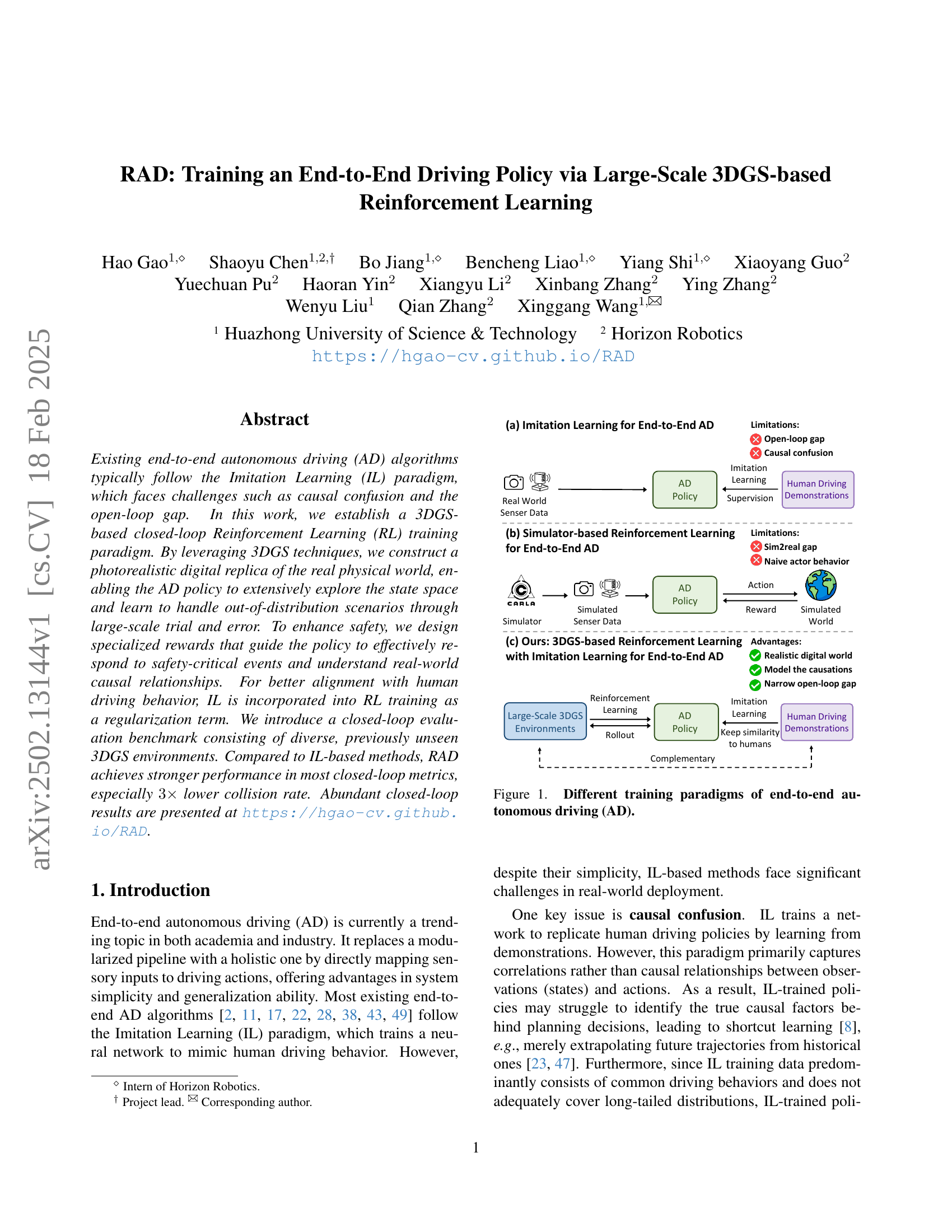
🔼 This figure compares three different training approaches for end-to-end autonomous driving models: Imitation Learning (IL), simulator-based Reinforcement Learning (RL), and the proposed 3DGS-based RL method. The IL approach uses human driving demonstrations to train the model, but suffers from causal confusion and an open-loop gap. The simulator-based RL approach addresses these issues by training in a simulator, but it introduces the Sim2Real gap and may not accurately model real-world conditions. The 3DGS-based RL approach combines the strengths of both methods, using a highly realistic digital replica of the real world to train the model via RL, while incorporating IL for better alignment with human driving behavior. This approach offers improved safety and addresses the limitations of the other two methods.
read the caption
Figure 1: Different training paradigms of end-to-end autonomous driving (AD).
| RL:IL | CR | DCR | SCR | DR | PDR | HDR | ADD | Long. Jerk | Lat. Jerk |
|---|---|---|---|---|---|---|---|---|---|
| 0:1 | 0.229 | 0.211 | 0.018 | 0.066 | 0.039 | 0.027 | 0.238 | 3.928 | 0.103 |
| 1:0 | 0.143 | 0.128 | 0.015 | 0.080 | 0.065 | 0.015 | 0.345 | 4.204 | 0.085 |
| 2:1 | 0.137 | 0.125 | 0.012 | 0.059 | 0.050 | 0.009 | 0.274 | 4.538 | 0.092 |
| 4:1 | 0.089 | 0.080 | 0.009 | 0.063 | 0.042 | 0.021 | 0.257 | 4.495 | 0.082 |
| 8:1 | 0.125 | 0.116 | 0.009 | 0.084 | 0.045 | 0.039 | 0.323 | 5.285 | 0.115 |
🔼 This table presents the results of an ablation study on the impact of different RL-to-IL step mixing ratios during the reinforced post-training stage of the RAD model. It shows how varying the proportion of reinforcement learning (RL) updates versus imitation learning (IL) updates affects various metrics, including collision rates, deviation ratios, jerk, and others, providing insights into the optimal balance between RL and IL for end-to-end autonomous driving.
read the caption
Table 1: Ablation on RL-to-IL step mixing ratios in the reinforced post-training stage.
In-depth insights#
3DGS-based RL#
The notion of ‘3DGS-based RL’ represents a significant advancement in training autonomous driving systems. By leveraging 3D Gaussian Splatting (3DGS), it constructs photorealistic digital replicas of real-world environments, enabling extensive exploration of state spaces otherwise inaccessible due to safety and cost constraints. This approach addresses limitations of Imitation Learning (IL) related to causal confusion and open-loop issues. Through large-scale trial and error within these realistic simulated environments, the agent can effectively learn to handle out-of-distribution scenarios and respond safely to critical events. The design of specialized rewards aligned with real-world causal relationships further refines the policy. Integrating IL as a regularization term during RL training helps align the agent’s behavior with that of human drivers.
RAD: End-to-End AD#
RAD: End-to-End AD signifies a pivotal shift towards holistic autonomous driving systems. This approach, contrasting with modular pipelines, promises system simplicity and enhanced generalization. By directly mapping sensory inputs to driving actions, it bypasses intermediate processing stages, potentially mitigating error propagation. The success hinges on robust neural networks capable of discerning complex relationships and generalizing across diverse scenarios. Challenges include ensuring safety, interpretability, and handling edge cases not well-represented in training data. RAD’s effectiveness relies on both the architecture and the data used for training. Significant research concentrates on enhancing network architectures to better capture intricate scene dynamics and devising innovative training methodologies to improve robustness and safety. The potential benefits include adaptive decision-making and greater autonomy in real-world driving conditions. The practicality of end-to-end AD hinges on surmounting challenges related to data bias, safety certification, and explainability in decision-making. Overcoming these is paramount for widespread adoption.
Causation Modeling#
Modeling causation in autonomous driving is paramount, moving beyond simple correlations to establish true cause-and-effect relationships. This is crucial for robust decision-making in unpredictable environments. Traditional imitation learning (IL) often falters here, as it primarily learns from observed data, capturing correlations that may not hold true in novel situations. A causation-aware model, on the other hand, can identify the true underlying factors influencing driving scenarios, leading to policies that generalize better and are more resilient to distributional shifts. Techniques like causal inference and intervention analysis could be incorporated to explicitly model causal relationships. This involves not only observing but also actively manipulating variables in a simulated environment to understand their true impact. Furthermore, counterfactual reasoning could be employed to assess the consequences of different actions in hypothetical scenarios, allowing the agent to learn from its mistakes without actually experiencing them in the real world. Prioritizing causation enables safer and more reliable autonomous systems.
RAD vs IL methods#
The paper posits that traditional Imitation Learning (IL) approaches, while simple, suffer from issues like causal confusion and an open-loop gap, hindering real-world deployment. RAD, the Reinforcement learning with imitation learning, addresses these limitations by enabling extensive exploration of the state space in a realistic simulated environment. This allows the AD policy to learn from its mistakes and handle out-of-distribution scenarios better, compared to IL which is limited by the training data. RAD also emphasizes safety-critical events and causal relationships through specialized rewards and constraints. The authors show RAD achieves a 3x lower collision rate compared to IL.
Safety by Design#
Safety by Design is a crucial element, particularly in the realm of autonomous systems. It requires proactive integration of safety considerations throughout the entire development lifecycle, not just as an afterthought. This encompasses various strategies, including fault tolerance, redundancy, and formal verification to minimize potential risks. The design must inherently consider potential failure modes and incorporate mechanisms to either prevent them or mitigate their impact, ensuring system-level safety. It also involves designing a system that can handle unforeseen situations, such as edge cases and black swan events, that may not be explicitly covered during training. Robustness and the ability to fail gracefully are essential attributes.
More visual insights#
More on figures

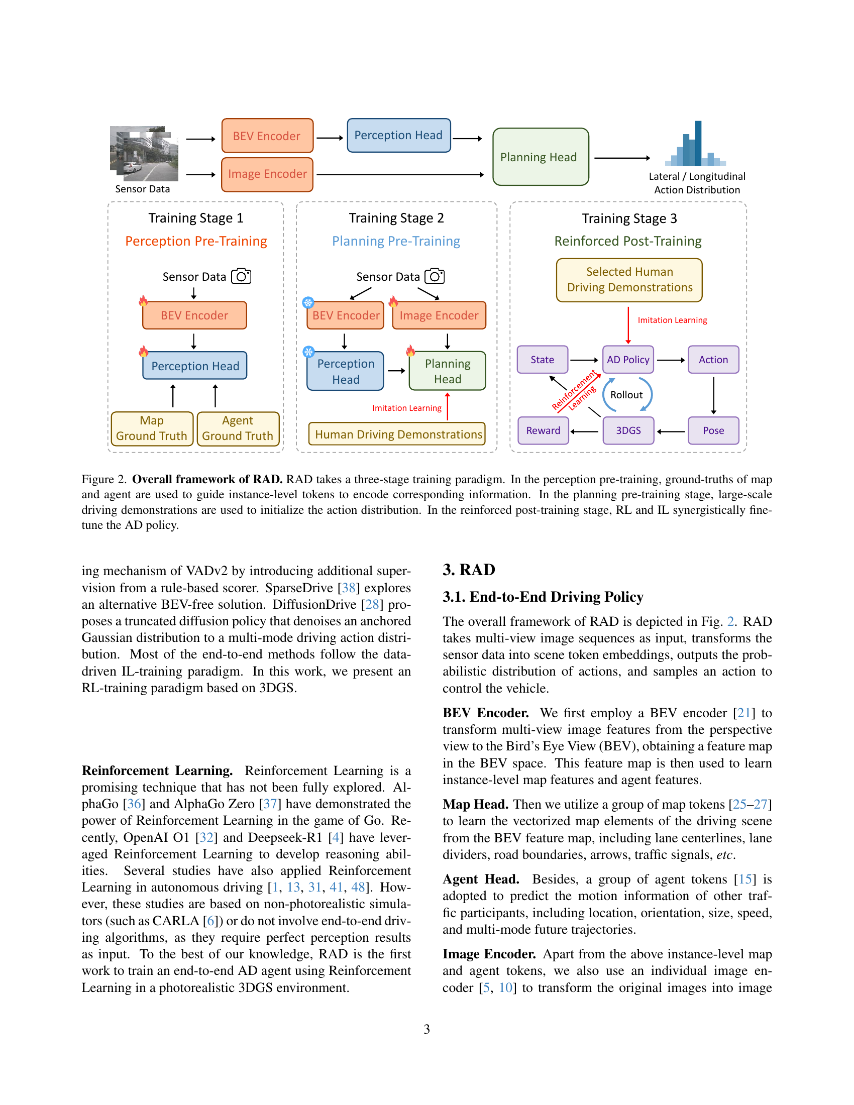
🔼 RAD’s training process consists of three stages. First, perception pre-training uses ground truth map and agent data to train instance-level token encoders for scene understanding. Second, planning pre-training leverages large-scale driving demonstrations to initialize the action distribution of the autonomous driving policy. Finally, reinforced post-training uses reinforcement learning (RL) and imitation learning (IL) together to fine-tune the policy, combining the strengths of both approaches to achieve optimal performance. RL handles the causal relationships and the open-loop problem, while IL maintains human-like driving behavior.
read the caption
Figure 2: Overall framework of RAD. RAD takes a three-stage training paradigm. In the perception pre-training, ground-truths of map and agent are used to guide instance-level tokens to encode corresponding information. In the planning pre-training stage, large-scale driving demonstrations are used to initialize the action distribution. In the reinforced post-training stage, RL and IL synergistically fine-tune the AD policy.

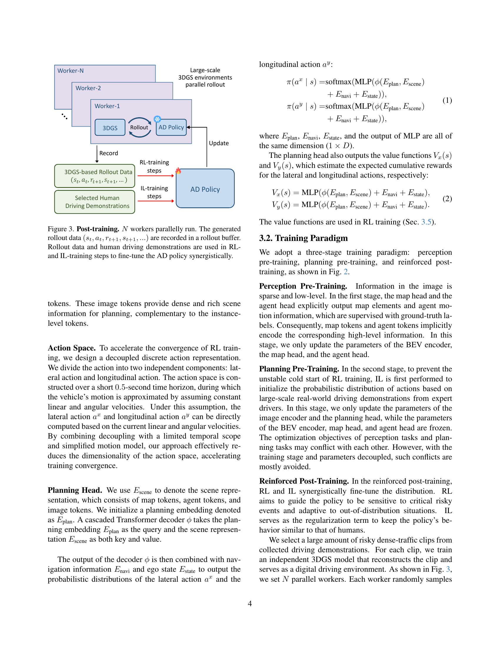
🔼 The figure illustrates the post-training stage of the RAD model, where N parallel workers simultaneously interact with the 3DGS environment. Each worker generates a sequence of data, including states (s), actions (a), rewards (r), and next states (s), which is then collected in a buffer. This data, along with human driving demonstrations, are used to refine the driving policy using both reinforcement learning (RL) and imitation learning (IL) techniques, combining their strengths for improved performance.
read the caption
Figure 3: Post-training. N𝑁Nitalic_N workers parallelly run. The generated rollout data (st,at,rt+1,st+1,…)subscript𝑠𝑡subscript𝑎𝑡subscript𝑟𝑡1subscript𝑠𝑡1…(s_{t},a_{t},r_{t+1},s_{t+1},...)( italic_s start_POSTSUBSCRIPT italic_t end_POSTSUBSCRIPT , italic_a start_POSTSUBSCRIPT italic_t end_POSTSUBSCRIPT , italic_r start_POSTSUBSCRIPT italic_t + 1 end_POSTSUBSCRIPT , italic_s start_POSTSUBSCRIPT italic_t + 1 end_POSTSUBSCRIPT , … ) are recorded in a rollout buffer. Rollout data and human driving demonstrations are used in RL- and IL-training steps to fine-tune the AD policy synergistically.

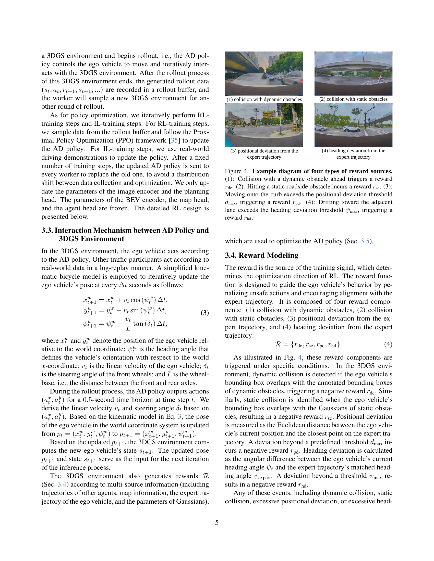
🔼 Figure 4 illustrates the four reward components used in the reinforcement learning process of the autonomous driving system. Each component penalizes specific unsafe behaviors: 1. Dynamic Collision (𝑟dcr_{ dc}): A negative reward is given if the vehicle collides with a moving obstacle (e.g., another car or pedestrian). 2. Static Collision (𝑟scr_{ sc}): A negative reward is given if the vehicle collides with a stationary obstacle (e.g., a curb or barrier). 3. Positional Deviation (𝑟pdr_{ pd}): A negative reward is given if the vehicle deviates from the optimal trajectory by more than a threshold distance (dmax). 4. Heading Deviation (𝑟hdr_{ hd}): A negative reward is given if the vehicle’s heading angle deviates from the optimal trajectory by more than a threshold angle (ψmax).
read the caption
Figure 4: Example diagram of four types of reward sources. (1): Collision with a dynamic obstacle ahead triggers a reward rdcsubscript𝑟dcr_{\text{dc}}italic_r start_POSTSUBSCRIPT dc end_POSTSUBSCRIPT. (2): Hitting a static roadside obstacle incurs a reward rscsubscript𝑟scr_{\text{sc}}italic_r start_POSTSUBSCRIPT sc end_POSTSUBSCRIPT. (3): Moving onto the curb exceeds the positional deviation threshold dmaxsubscript𝑑maxd_{\text{max}}italic_d start_POSTSUBSCRIPT max end_POSTSUBSCRIPT, triggering a reward rpdsubscript𝑟pdr_{\text{pd}}italic_r start_POSTSUBSCRIPT pd end_POSTSUBSCRIPT. (4): Drifting toward the adjacent lane exceeds the heading deviation threshold ψmaxsubscript𝜓max\psi_{\text{max}}italic_ψ start_POSTSUBSCRIPT max end_POSTSUBSCRIPT, triggering a reward rhdsubscript𝑟hdr_{\text{hd}}italic_r start_POSTSUBSCRIPT hd end_POSTSUBSCRIPT.

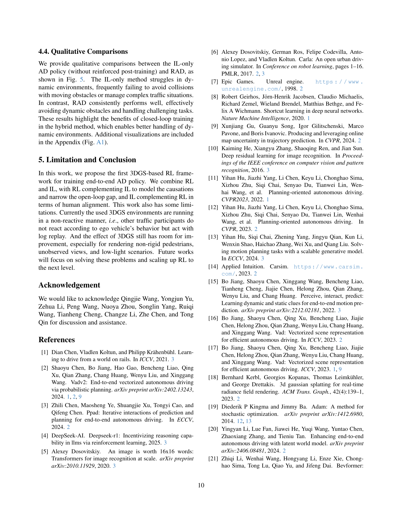
🔼 This figure presents a qualitative comparison of the performance of an Imitation Learning (IL)-only policy versus the proposed RAD policy in handling complex driving scenarios within a 3DGS (3D Gaussian Splatting) simulated environment. The scenarios depicted showcase the challenges of yielding to pedestrians (Rows 1-2) and executing unprotected left turns (Rows 3-4). By visually comparing the behaviors of both policies under these conditions, the figure highlights RAD’s superior ability to navigate these complex situations safely and smoothly, while the IL-only approach demonstrates limitations in handling such challenging conditions.
read the caption
Figure 5: Closed-loop qualitative comparisons between the IL-only policy and RAD in 3DGS environments. Rows 1-2 correspond to Yield to Pedestrians. Rows 3-4 correspond to Unprotected Left-turn.

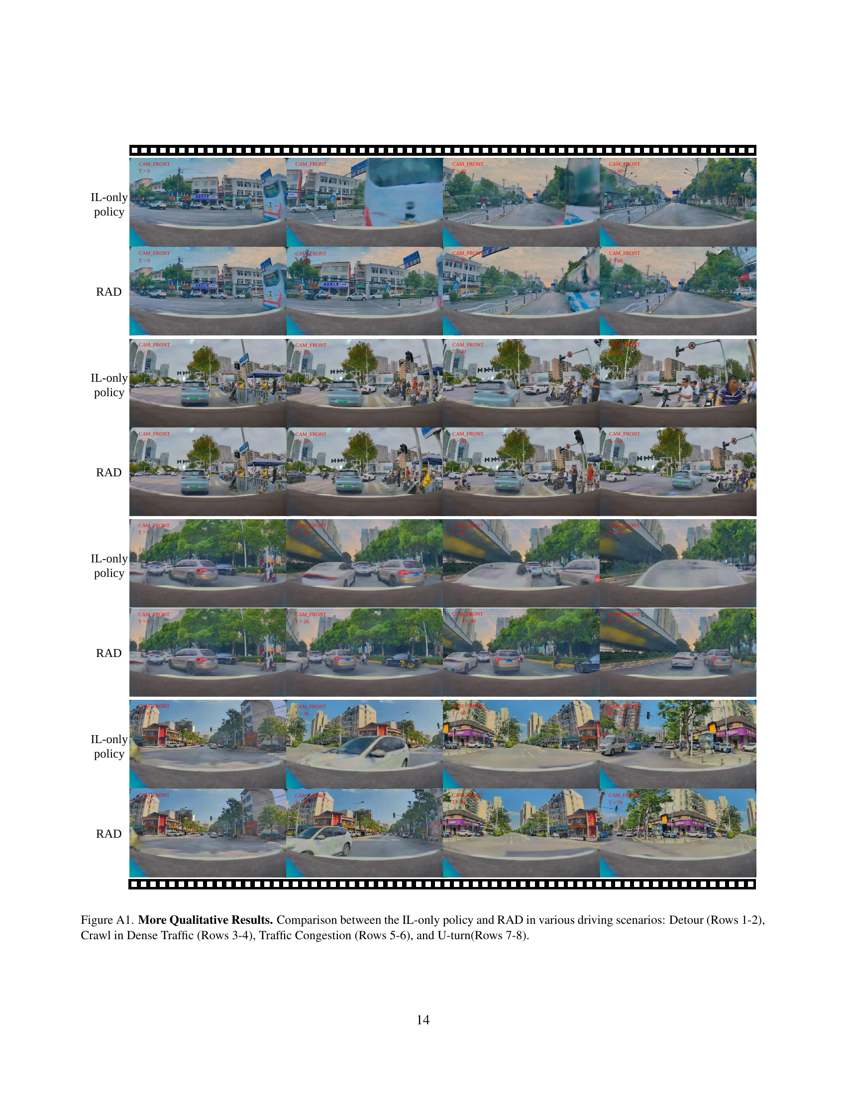
🔼 Figure A1 presents a qualitative comparison of the performance of the IL-only policy and RAD across diverse driving scenarios. The scenarios are displayed in rows, with each row showcasing a different driving situation. Rows 1-2 illustrate a detour maneuver; Rows 3-4 show navigation through dense traffic conditions; Rows 5-6 depict maneuvering through congested traffic; and Rows 7-8 demonstrate successful U-turn execution. For each scenario, the figure displays a sequence of images, allowing visual comparison between the IL-only policy’s and RAD’s performance in terms of smoothness, collision avoidance, and adherence to the driving lanes.
read the caption
Figure A1: More Qualitative Results. Comparison between the IL-only policy and RAD in various driving scenarios: Detour (Rows 1-2), Crawl in Dense Traffic (Rows 3-4), Traffic Congestion (Rows 5-6), and U-turn(Rows 7-8).
More on tables
| ID | Dynamic | Static | Position | Heading | CR | DCR | SCR | DR | PDR | HDR | ADD | Long. Jerk | Lat. Jerk |
|---|---|---|---|---|---|---|---|---|---|---|---|---|---|
| Collision | Collision | Deviation | Deviation | ||||||||||
| 1 | ✓ | 0.172 | 0.154 | 0.018 | 0.092 | 0.033 | 0.059 | 0.259 | 4.211 | 0.095 | |||
| 2 | ✓ | ✓ | ✓ | 0.238 | 0.217 | 0.021 | 0.090 | 0.045 | 0.045 | 0.241 | 3.937 | 0.098 | |
| 3 | ✓ | ✓ | ✓ | 0.146 | 0.128 | 0.018 | 0.060 | 0.030 | 0.030 | 0.263 | 3.729 | 0.083 | |
| 4 | ✓ | ✓ | ✓ | 0.151 | 0.142 | 0.009 | 0.069 | 0.042 | 0.027 | 0.303 | 3.938 | 0.079 | |
| 5 | ✓ | ✓ | ✓ | 0.166 | 0.157 | 0.009 | 0.048 | 0.036 | 0.012 | 0.243 | 3.334 | 0.067 | |
| 6 | ✓ | ✓ | ✓ | ✓ | 0.089 | 0.080 | 0.009 | 0.063 | 0.042 | 0.021 | 0.257 | 4.495 | 0.082 |
🔼 This table presents the results of an ablation study on the reward components used in the RAD model. Each row represents a different configuration, where certain reward components are either included or excluded. The impact of each component on various performance metrics (CR, DCR, SCR, DR, PDR, HDR, ADD, Long. Jerk, Lat. Jerk) is assessed. The goal is to determine the contribution of each reward component in achieving optimal performance, particularly in minimizing collisions and improving the smoothness of driving behavior.
read the caption
Table 2: Ablation on reward sources. The table shows the impact of different reward components on performance.
| ID | PPO Obj. | Dynamic Col. | Static Col. | Position Dev. | Heading Dev. | CR | DCR | SCR | DR | PDR | HDR | ADD | Long. Jerk | Lat. Jerk |
|---|---|---|---|---|---|---|---|---|---|---|---|---|---|---|
| Auxiliary Obj. | Auxiliary Obj. | Auxiliary Obj. | Auxiliary Obj. | |||||||||||
| 1 | ✓ | 0.249 | 0.223 | 0.026 | 0.077 | 0.047 | 0.030 | 0.266 | 4.209 | 0.104 | ||||
| 2 | ✓ | ✓ | 0.178 | 0.163 | 0.015 | 0.151 | 0.101 | 0.050 | 0.301 | 3.906 | 0.085 | |||
| 3 | ✓ | ✓ | ✓ | ✓ | 0.137 | 0.125 | 0.012 | 0.157 | 0.145 | 0.012 | 0.296 | 3.419 | 0.071 | |
| 4 | ✓ | ✓ | ✓ | ✓ | 0.169 | 0.151 | 0.018 | 0.075 | 0.042 | 0.033 | 0.254 | 4.450 | 0.098 | |
| 5 | ✓ | ✓ | ✓ | ✓ | 0.149 | 0.134 | 0.015 | 0.063 | 0.057 | 0.006 | 0.324 | 3.980 | 0.086 | |
| 6 | ✓ | ✓ | ✓ | ✓ | 0.128 | 0.119 | 0.009 | 0.066 | 0.030 | 0.036 | 0.254 | 4.102 | 0.092 | |
| 7 | ✓ | ✓ | ✓ | ✓ | 0.187 | 0.175 | 0.012 | 0.077 | 0.056 | 0.021 | 0.309 | 5.014 | 0.112 | |
| 8 | ✓ | ✓ | ✓ | ✓ | ✓ | 0.089 | 0.080 | 0.009 | 0.063 | 0.042 | 0.021 | 0.257 | 4.495 | 0.082 |
🔼 This ablation study analyzes the effects of each auxiliary objective (dynamic collision avoidance, static collision avoidance, positional deviation correction, and heading deviation correction) on the overall performance of the autonomous driving policy. It shows how each component contributes to the final results, highlighting their importance in collision avoidance, trajectory tracking, and driving smoothness.
read the caption
Table 3: Ablation on auxiliary objectives. The table shows the impact of different auxiliary objectives on performance.
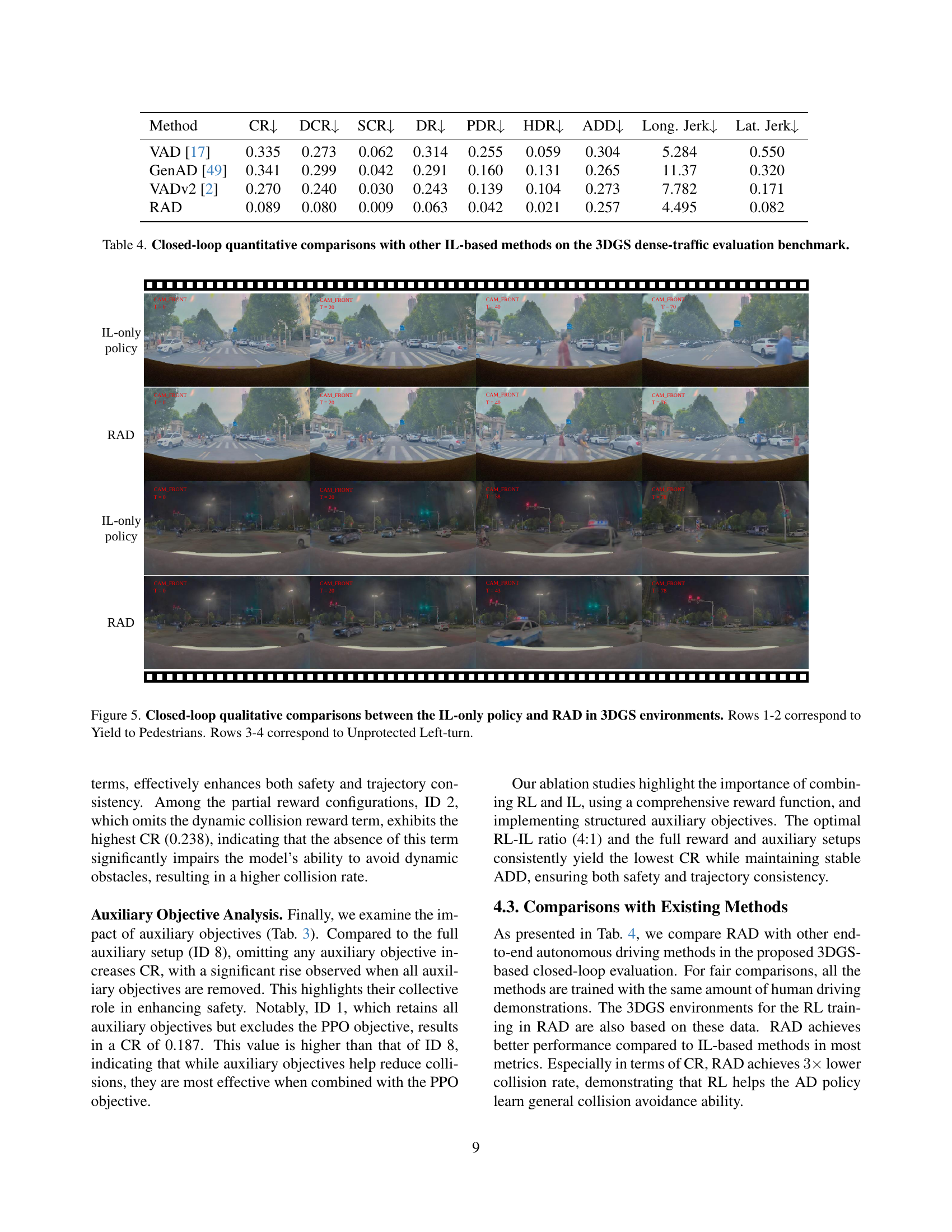
| Method | CR | DCR | SCR | DR | PDR | HDR | ADD | Long. Jerk | Lat. Jerk |
|---|---|---|---|---|---|---|---|---|---|
| VAD [17] | 0.335 | 0.273 | 0.062 | 0.314 | 0.255 | 0.059 | 0.304 | 5.284 | 0.550 |
| GenAD [49] | 0.341 | 0.299 | 0.042 | 0.291 | 0.160 | 0.131 | 0.265 | 11.37 | 0.320 |
| VADv2 [2] | 0.270 | 0.240 | 0.030 | 0.243 | 0.139 | 0.104 | 0.273 | 7.782 | 0.171 |
| RAD | 0.089 | 0.080 | 0.009 | 0.063 | 0.042 | 0.021 | 0.257 | 4.495 | 0.082 |
🔼 This table presents a quantitative comparison of various end-to-end autonomous driving (AD) methods, specifically focusing on those that utilize Imitation Learning (IL). The comparison is based on performance metrics obtained from a rigorous evaluation benchmark involving dense traffic scenarios within a photorealistic 3DGS (3D Gaussian Splatting) simulated environment. The metrics assess collision rates (both dynamic and static), positional and heading deviations from expert trajectories, average deviation distance, and longitudinal and lateral jerk. These metrics provide a comprehensive evaluation of safety, accuracy, and smoothness of the AD policies in challenging driving conditions.
read the caption
Table 4: Closed-loop quantitative comparisons with other IL-based methods on the 3DGS dense-traffic evaluation benchmark.
| config | Planning Pre-Training |
|---|---|
| learning rate | 1e-4 |
| learning rate schedule | cosine decay |
| optimizer | AdamW [19, 30] |
| optimizer hyper-parameters | , , = 0.9, 0.999, 1e-8 |
| weight decay | 1e-4 |
| batch size | 512 |
| training steps | 30k |
| planning head dim | 256 |
🔼 This table lists the hyperparameters used in the Planning Pre-training stage of the RAD model. It includes the learning rate, learning rate schedule, optimizer, optimizer hyperparameters, weight decay, batch size, and the number of training steps. The dimensions of the planning head are also specified.
read the caption
Table A1: Hyperparameters used in RAD Planning Pre-Training stage.
| config | Reinforced Post-Training |
|---|---|
| learning rate | 5e-6 |
| learning rate schedule | cosine decay |
| optimizer | AdamW [19, 30] |
| optimizer hyper-parameters | , , = 0.9, 0.999, 1e-8 |
| weight decay | 1e-4 |
| RL worker number | 32 |
| RL batch size | 32 |
| IL batch size | 128 |
| GAE parameter | , |
| clipping thresholds | , |
| deviation threshold | , |
| planning head dim | 256 |
| value function dim | 256 |
🔼 This table lists the hyperparameters used during the reinforced post-training stage of the RAD model. It includes the learning rate and its decay schedule, the optimizer used (AdamW), optimizer hyperparameters (beta1, beta2, epsilon), weight decay, the number of RL workers, RL and IL batch sizes, the GAE parameter (gamma and lambda), clipping thresholds (epsilon_x and epsilon_y), the maximum deviation threshold (dmax and vmax), planning and value function dimensions. These settings are crucial for fine-tuning the model’s policy using both reinforcement and imitation learning.
read the caption
Table A2: Hyperparameters used in RAD Reinforced Post-Training stage.
Full paper#