TL;DR#
Semi-supervised heterogeneous domain adaptation (SHDA) tackles learning across different data types and distributions, but the nature of knowledge transfer remains unclear. This paper investigates this issue, revealing that characteristics of source data like category and feature information don’t greatly affect target domain performance. Surprisingly, even noise can be useful source! The study employs two supervised learning methods and seven SHDA techniques on approximately 330 SHDA tasks, challenging traditional assumptions about informative source data. These counter-intuitive findings are very novel.
The key to unlocking knowledge transfer in SHDA lies in the transferability and discriminability of the source domain itself. To illustrate the discovery, the paper introduces a unified Knowledge Transfer Framework (KTF) and designs experiments with various noise domains. The study finds that ensuring these properties in source samples boosts knowledge transfer, regardless of their origin (image, text, noise). Datasets and codes are publicly available, encouraging further research.
Key Takeaways#
Why does it matter?#
This paper offers a new perspective on SHDA by demonstrating noise as a valuable resource for knowledge transfer. This finding challenges conventional views and has potential to inspire novel DA algorithms, ultimately advancing machine learning research and applications in heterogeneous domains.
Visual Insights#

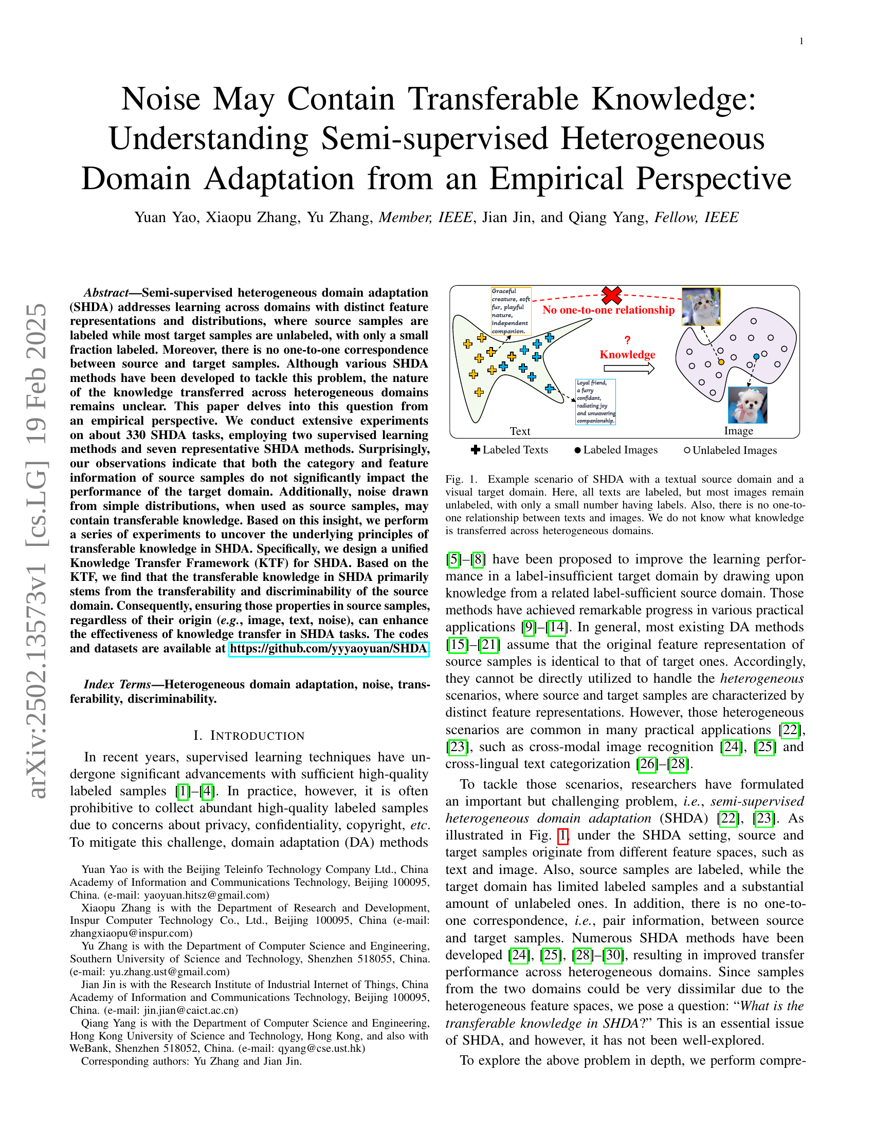
🔼 This figure illustrates a common scenario in semi-supervised heterogeneous domain adaptation (SHDA). A textual source domain (e.g., labeled descriptions of animals) and a visual target domain (e.g., images of animals, some labeled, most unlabeled) are shown. The key aspects highlighted are: the difference in data representation between the domains (text vs. images), the semi-supervised nature of the target domain (mostly unlabeled data), and the absence of a direct correspondence between source and target samples (no pairwise links between specific text descriptions and images). The overall question posed is: what type of knowledge successfully transfers from the text to the image domain in this situation?
read the caption
Figure 1: Example scenario of SHDA with a textual source domain and a visual target domain. Here, all texts are labeled, but most images remain unlabeled, with only a small number having labels. Also, there is no one-to-one relationship between texts and images. We do not know what knowledge is transferred across heterogeneous domains.
| Notation | Description |
|---|---|
| / | Source/Target feature space |
| / | Source/Target domain |
| / | Labeled/Unlabeled target domain |
| / / | the -th sample in / / |
| / | One-hot label of / |
| / / | Number of samples in / / |
| Number of categories |
🔼 This table lists the notations used throughout the paper. It defines the symbols for key concepts such as source and target domains, labeled and unlabeled data, feature spaces, and the number of samples and categories.
read the caption
TABLE I: Notations.
In-depth insights#
SHDA’s Noise Core#
The core idea revolves around transferable knowledge in semi-supervised heterogeneous domain adaptation (SHDA), questioning traditional reliance on source data’s semantic relevance. Instead, noise, surprisingly, can be a potent source of transferable knowledge. The emphasis shifts to the transferability and discriminability of the noise domain itself. The research highlights the importance of properties within the noise, rather than its origin, redefining knowledge transfer in SHDA. The study challenges existing assumptions and opens new avenues for leveraging noise in domain adaptation.
KTF for SHDA#
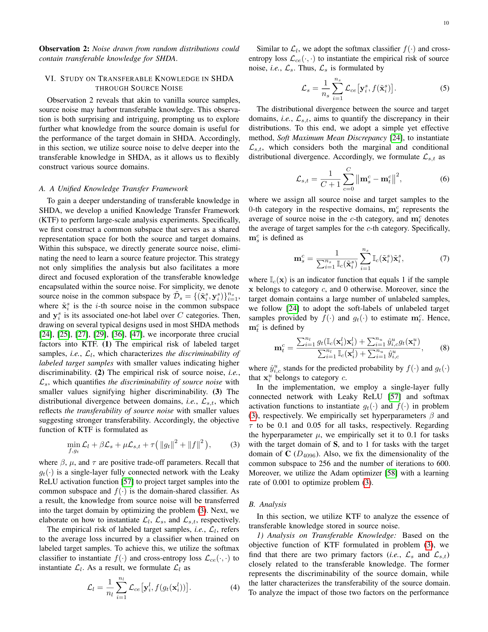
The Knowledge Transfer Framework (KTF) for Semi-supervised Heterogeneous Domain Adaptation (SHDA) seems like a crucial component for understanding knowledge transfer. The framework likely aims to create a unified space for source and target domains, enabling a more direct analysis of transferable knowledge within source noise. By constructing a common subspace and generating source noise directly, the authors eliminate the need for learning a source feature projector, simplifying analysis and focusing on the essence of transferable knowledge. KTF incorporates factors like the empirical risk of labeled target samples (discriminability), the empirical risk of source noise (discriminability), and the distributional divergence between domains (transferability). The formulation of KTF’s objective function, likely a minimization problem balancing these factors, would be essential for guiding the transfer process. This unified approach allows systematic manipulation and study of noise characteristics and their influence on target domain performance. The use of a softmax classifier, cross-entropy loss, and soft maximum mean discrepancy (MMD) indicates a standard yet effective approach to knowledge transfer in KTF.
Transferability Core#
The paper empirically investigates transferable knowledge in semi-supervised heterogeneous domain adaptation (SHDA). A key finding is that noise from simple distributions can transfer knowledge, challenging the reliance on vanilla source samples. The category and feature information of source samples are surprisingly less influential. A unified Knowledge Transfer Framework (KTF) is introduced, revealing that transferable knowledge stems from the source domain’s transferability and discriminability. Regardless of the data origin (image, text, noise), ensuring these properties in source samples boosts SHDA effectiveness. The research highlights noise as a valuable resource and emphasizes the importance of transferability and discriminability rather than specific source data characteristics. It offers a new perspective on domain adaptation, applicable in scenarios with limited access to source data.
Domain Alignment#
Domain alignment is a crucial aspect of domain adaptation, particularly in heterogeneous scenarios where feature spaces differ. Effective alignment seeks to bridge the gap between source and target data distributions, enabling knowledge transfer. Approaches often involve learning feature transformations or projecting data into a shared subspace, thereby minimizing distributional divergence. Marginal and conditional distribution alignment are key strategies. Additionally, methods focusing on aligning category-level representations or utilizing pseudo-labels for unlabeled target data have shown promise. Addressing the challenge of negative transfer and ensuring discriminability within the aligned space remain important research directions to enhance the robustness and effectiveness of domain alignment techniques.
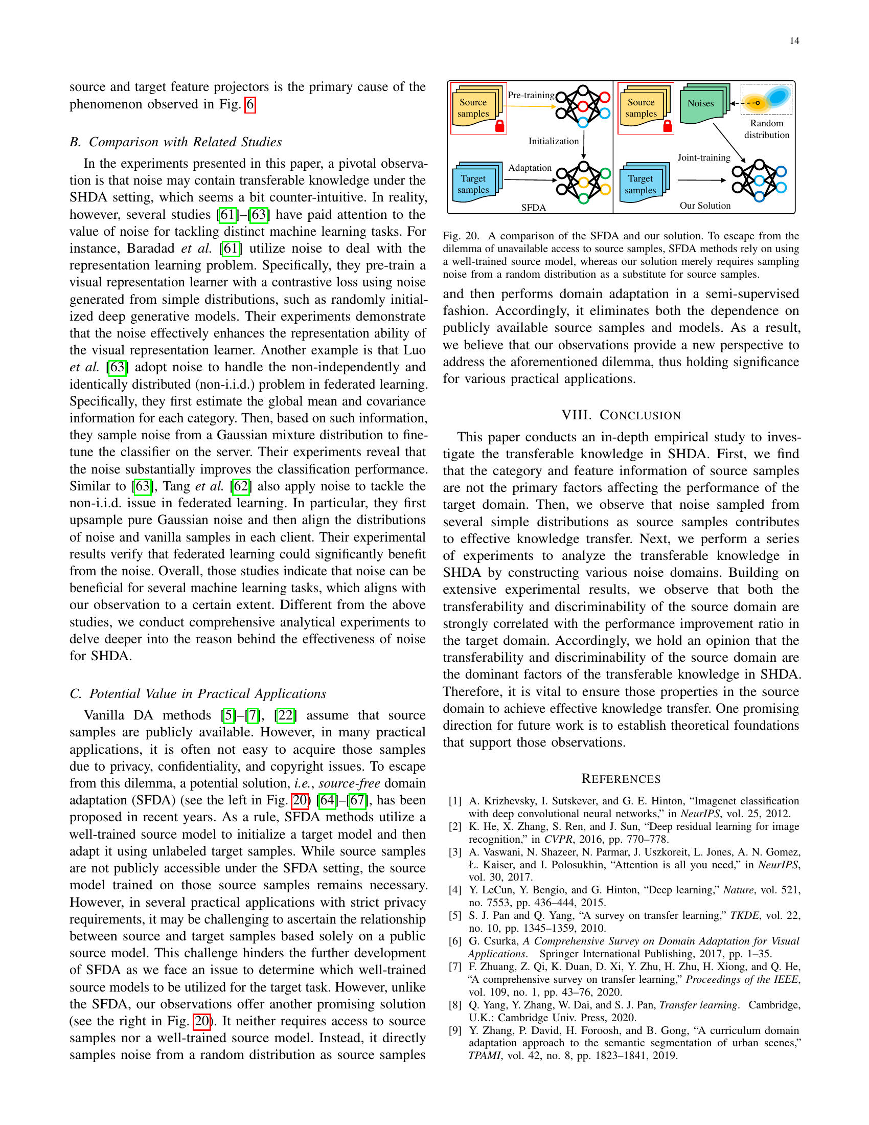
SFDA Alternative#
The “SFDA Alternative” presents a compelling approach by sampling noise from random distributions as source samples, bypassing the need for real-world data. This is advantageous in scenarios where data is restricted due to privacy, confidentiality, or copyright. Domain adaptation is done in a semi-supervised manner after noise is sampled for source training. The focus on simple distribution of noise eliminates the need of carefully curate source data and maintains privacy. Furthermore, it removes the need to identify the perfect domain and train on that domain for transfer learning. Finally, it reduces dependency on publicly available samples.
More visual insights#
More on figures

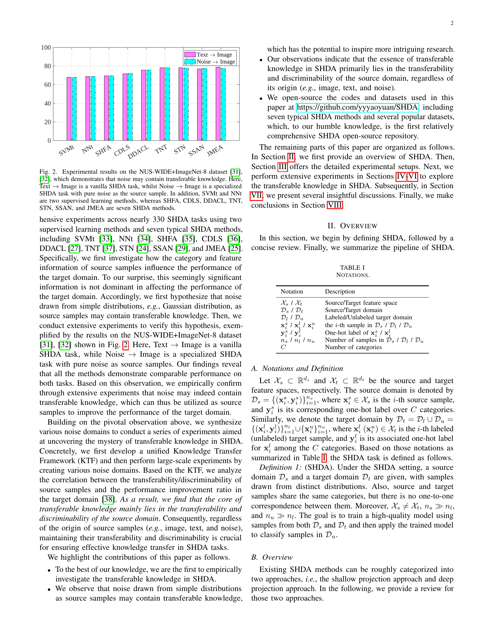
🔼 Figure 2 presents a comparative analysis of various domain adaptation methods’ performance on the NUS-WIDE+ImageNet-8 dataset. Two scenarios are compared: a standard semi-supervised heterogeneous domain adaptation (SHDA) task (‘Text → Image’), and a novel task (‘Noise → Image’) where synthetic noise replaces the actual source data. The figure showcases the performance of two supervised learning methods (SVMt, NNt) and seven SHDA methods (SHFA, CDLS, DDACL, TNT, STN, SSAN, JMEA). The results surprisingly show comparable performance between the standard SHDA task and the noise-based task, suggesting that noise itself may contain transferable knowledge in the context of SHDA.
read the caption
Figure 2: Experimental results on the NUS-WIDE+ImageNet-8 dataset [31, 32], which demonstrates that noise may contain transferable knowledge. Here, Text →→\rightarrow→ Image is a vanilla SHDA task, whilst Noise →→\rightarrow→ Image is a specialized SHDA task with pure noise as the source sample. In addition, SVMt and NNt are two supervised learning methods, whereas SHFA, CDLS, DDACL, TNT, STN, SSAN, and JMEA are seven SHDA methods.

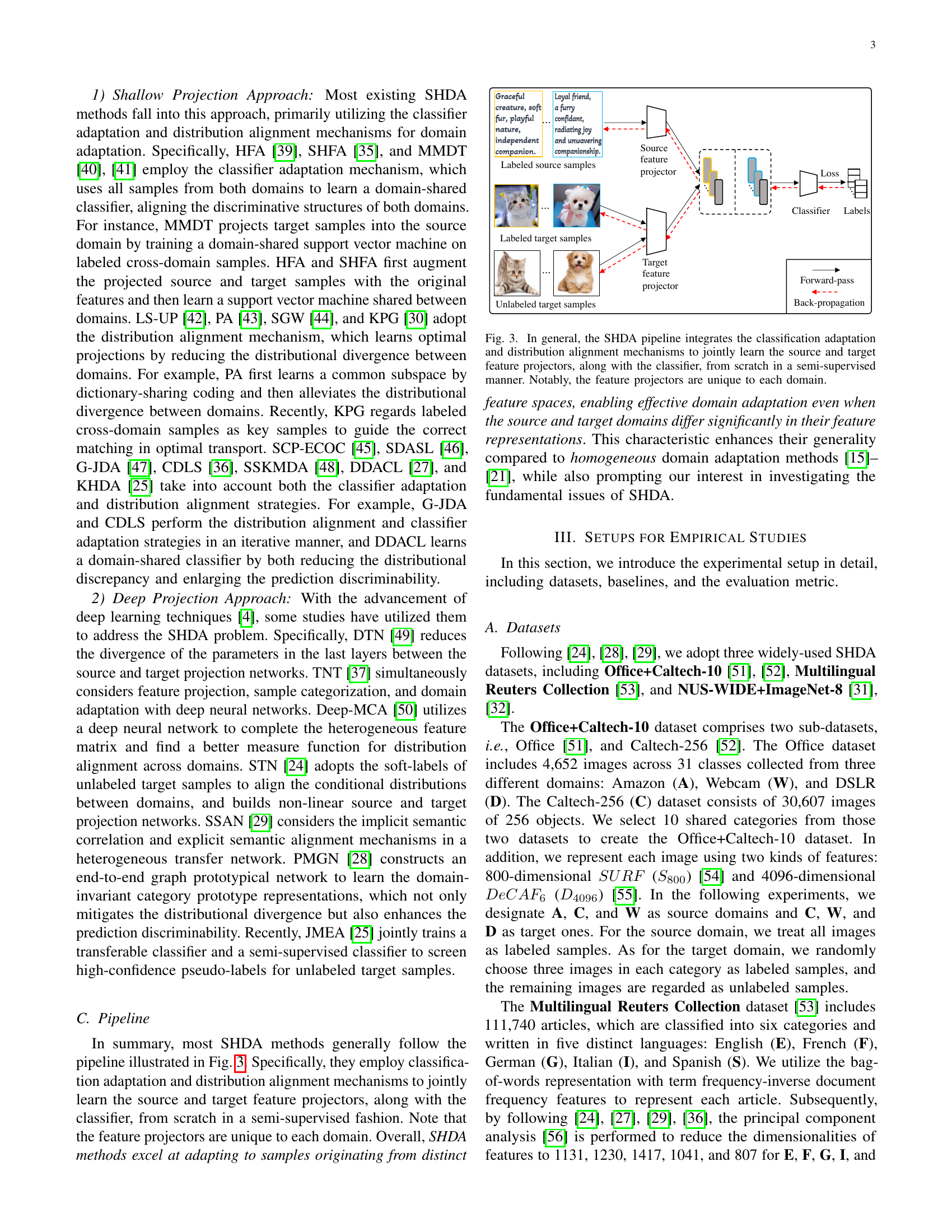
🔼 The figure illustrates the typical pipeline of semi-supervised heterogeneous domain adaptation (SHDA) methods. It shows how SHDA approaches use both classification adaptation (adjusting the classifier to handle the differences between domains) and distribution alignment (making the distributions of source and target data more similar) to learn feature projectors (functions that transform data from each domain into a common space) and a shared classifier. The key point is that the feature projectors are specific to each domain (source and target), reflecting the differences in their data representations. This process allows the algorithm to effectively learn from labeled source data and a mix of labeled and unlabeled target data, even though the data across domains is not directly comparable.
read the caption
Figure 3: In general, the SHDA pipeline integrates the classification adaptation and distribution alignment mechanisms to jointly learn the source and target feature projectors, along with the classifier, from scratch in a semi-supervised manner. Notably, the feature projectors are unique to each domain.

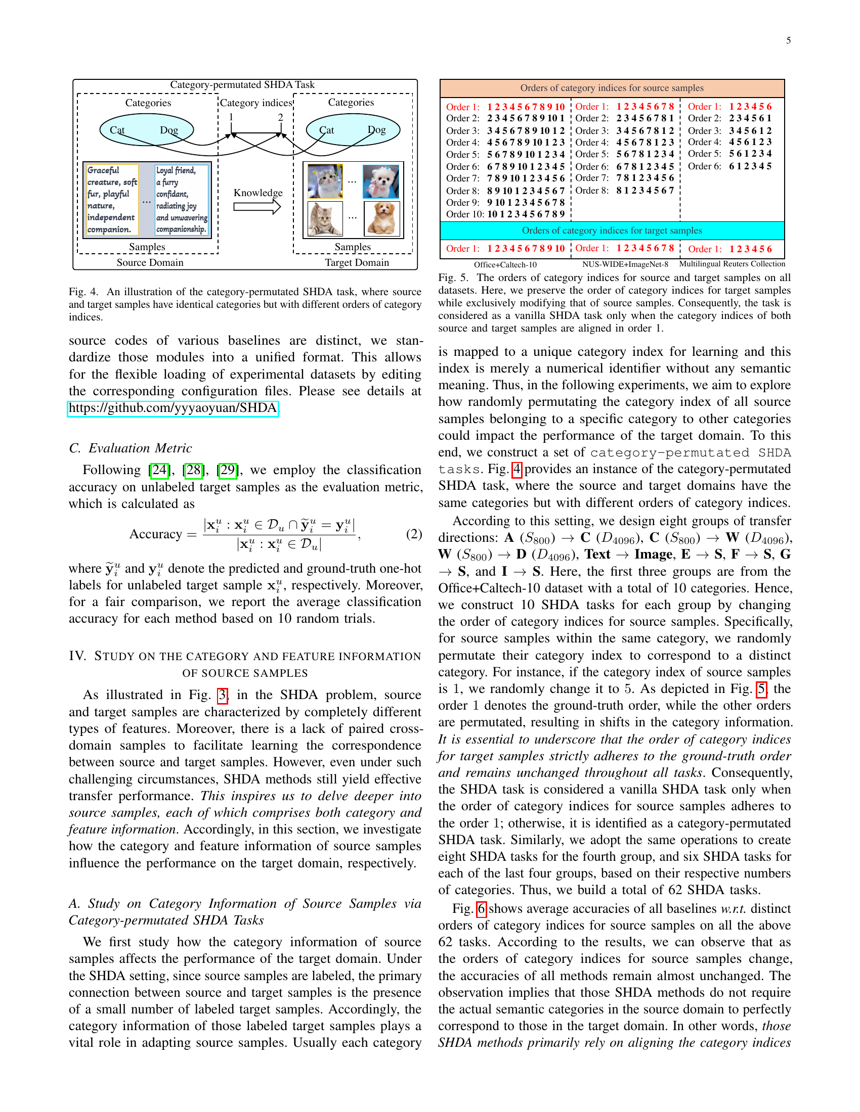
🔼 This figure illustrates a scenario in semi-supervised heterogeneous domain adaptation (SHDA). It shows how the order of category indices can differ between the source and target domains, even though the categories themselves are the same. The source domain has labeled samples, while the target domain has both labeled and unlabeled samples. This setup is used to investigate how the ordering of categories affects the performance of SHDA methods.
read the caption
Figure 4: An illustration of the category-permutated SHDA task, where source and target samples have identical categories but with different orders of category indices.

🔼 This figure shows how the order of categories affects the performance of semi-supervised heterogeneous domain adaptation (SHDA) tasks. Across three datasets (Office+Caltech-10, Multilingual Reuters Collection, and NUS-WIDE+ImageNet-8), the order of category indices for target samples remains consistent, while the order of categories in the source samples is systematically permuted. Each permutation represents a separate SHDA task. The original, unpermuted order (Order 1) represents a standard SHDA task; all other permutations represent variations where the source category order is shuffled. This experimental design allows researchers to isolate and analyze the impact of the source data’s category order on SHDA performance.
read the caption
Figure 5: The orders of category indices for source and target samples on all datasets. Here, we preserve the order of category indices for target samples while exclusively modifying that of source samples. Consequently, the task is considered as a vanilla SHDA task only when the category indices of both source and target samples are aligned in order 1.

🔼 This figure shows the classification accuracy results for different methods on a semi-supervised heterogeneous domain adaptation task. The task involves transferring knowledge from the Amazon (A) domain with 800-dimensional SURF features to the Caltech-256 (C) domain with 4096-dimensional DeCAF6 features. The x-axis represents different orders of category indices for the source domain samples, demonstrating the impact of varying category information on the adaptation performance. The y-axis represents the classification accuracy. Different colored lines represent various SHDA methods, and the impact of the different methods can be compared against two supervised methods (SVM and NN). The results are compared across different orderings of categories to show that the category ordering does not greatly influence results.
read the caption
(a) A (S800subscript𝑆800S_{800}italic_S start_POSTSUBSCRIPT 800 end_POSTSUBSCRIPT) →→\rightarrow→C (D4096subscript𝐷4096D_{4096}italic_D start_POSTSUBSCRIPT 4096 end_POSTSUBSCRIPT)

🔼 This figure shows the classification accuracy results for a semi-supervised heterogeneous domain adaptation (SHDA) task. Specifically, it illustrates the performance of various SHDA methods when adapting from a source domain with SURF features (S800) in the Caltech-256 dataset (C) to a target domain with DeCAF features (D4096) in the Webcam dataset (W). The x-axis represents different permutations of category indices in the source domain, while the y-axis shows the classification accuracy. The purpose is to investigate the impact of category information ordering in the source data on the effectiveness of SHDA.
read the caption
(b) C (S800subscript𝑆800S_{800}italic_S start_POSTSUBSCRIPT 800 end_POSTSUBSCRIPT) →→\rightarrow→ W (D4096subscript𝐷4096D_{4096}italic_D start_POSTSUBSCRIPT 4096 end_POSTSUBSCRIPT)

🔼 This figure shows the results of a semi-supervised heterogeneous domain adaptation (SHDA) experiment. Specifically, it visualizes the classification accuracy across different orderings of category indices in the source domain samples. The experiment uses a Webcam (W) domain with SURF features (S800) as the source domain and a DSLR (D) domain with DeCAF features (D4096) as the target domain. The x-axis represents the different orderings, and the y-axis represents the classification accuracy. This helps to understand the impact of category information order in source data on the SHDA performance. Different SHDA algorithms are likely compared in the figure, although the algorithms are not explicitly mentioned in the given caption.
read the caption
(c) W (S800subscript𝑆800S_{800}italic_S start_POSTSUBSCRIPT 800 end_POSTSUBSCRIPT) →→\rightarrow→D (D4096subscript𝐷4096D_{4096}italic_D start_POSTSUBSCRIPT 4096 end_POSTSUBSCRIPT)

🔼 This figure shows the experimental results on the NUS-WIDE+ImageNet-8 dataset. It compares the performance of various semi-supervised heterogeneous domain adaptation (SHDA) methods and two supervised learning methods (SVMt and NNt) on a text-to-image domain adaptation task. The results show that using pure noise as source samples does not significantly impair the performance compared to using actual text data as the source.
read the caption
(d) Text→→\rightarrow→Image

🔼 This figure shows the classification accuracy for different methods across various orders of category indices in a semi-supervised heterogeneous domain adaptation (SHDA) task. The specific task shown is the transfer from English (E) to Spanish (S) domains, where English is the source domain and Spanish is the target domain. The x-axis represents the order of category indices for source samples, and the y-axis represents the classification accuracy. Different colored lines represent different SHDA methods used in the study.
read the caption
(e) E→→\rightarrow→S

🔼 This figure shows the classification accuracy for different orders of category indices in source samples for a semi-supervised heterogeneous domain adaptation task. The task involves adapting from the French (F) language domain to the Spanish (S) language domain. The x-axis represents different permutations of category indices (order 1 is the original order), and the y-axis shows the classification accuracy. Multiple lines represent different domain adaptation methods.
read the caption
(f) F→→\rightarrow→S

🔼 This figure shows the classification accuracy results for various domain adaptation methods on a semi-supervised heterogeneous domain adaptation (SHDA) task. The specific task depicted is transferring knowledge from the German (G) language domain to the Spanish (S) language domain. The x-axis represents different permutations of the category indices in the source domain (German), while the y-axis shows the classification accuracy. Each line represents a different domain adaptation method, illustrating their performance under various category index orderings. The purpose is to analyze how the category information in the source domain impacts the accuracy of the model.
read the caption
(g) G→→\rightarrow→S

🔼 This figure shows the classification accuracy for different methods across various orders of category indices for source samples in a semi-supervised heterogeneous domain adaptation (SHDA) task where Italian (I) is the source domain and Spanish (S) is the target domain. The experiment permutes the order of categories in the source domain while keeping the target domain’s category order constant to analyze how category order impacts performance. The goal is to understand the impact of category information from the source domain on the target domain in SHDA.
read the caption
(h) I→→\rightarrow→S

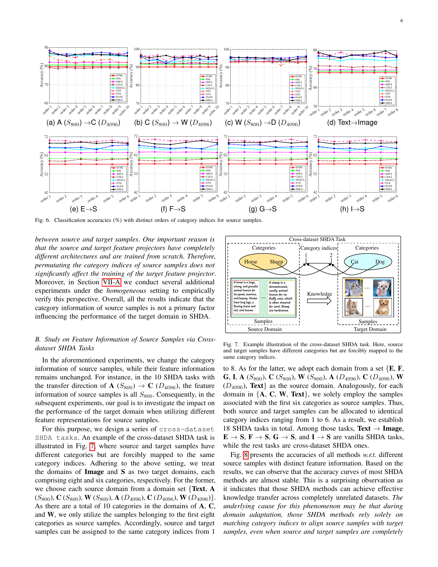
🔼 Figure 6 presents the results of an experiment investigating how the order of category indices in source samples affects the performance of various SHDA methods on eight different transfer tasks. The x-axis represents the different permutation orders of category indices for source samples (Order 1 being the original order), while the y-axis displays the classification accuracy. The results show that permuting the category indices of source samples has minimal impact on the performance of various SHDA methods, suggesting that the exact alignment of source and target category labels is not crucial for effective SHDA.
read the caption
Figure 6: Classification accuracies (%) with distinct orders of category indices for source samples.

🔼 This figure illustrates a scenario in semi-supervised heterogeneous domain adaptation (SHDA). It demonstrates the challenge of adapting between domains where source and target data have different underlying categories (e.g., different types of features). The key point is that, despite the different original categories, a mapping is artificially imposed to force the categories to align numerically. This highlights the difficulty of SHDA, which requires adaptation despite the lack of a natural one-to-one correspondence between source and target categories.
read the caption
Figure 7: Example illustration of the cross-dataset SHDA task. Here, source and target samples have different categories but are forcibly mapped to the same category indices.

🔼 The figure shows the classification accuracies of different machine learning methods when using various types of source samples for the image domain in semi-supervised heterogeneous domain adaptation (SHDA). The x-axis represents different types of source samples, while the y-axis represents the classification accuracy. Different colors represent different SHDA methods. The figure demonstrates that using noise samples, as opposed to traditional source data, can achieve similar or even better performance in SHDA tasks.
read the caption
(a) Target domain: Image

🔼 The figure shows the classification accuracies achieved by different methods when various proportions of noises are injected into source samples in semi-supervised heterogeneous domain adaptation (SHDA) tasks. The target domain is S. The x-axis represents different proportions of noise, and the y-axis represents classification accuracy. Each line corresponds to a different SHDA method, including supervised learning methods and several typical SHDA methods.
read the caption
(b) Target domain: S

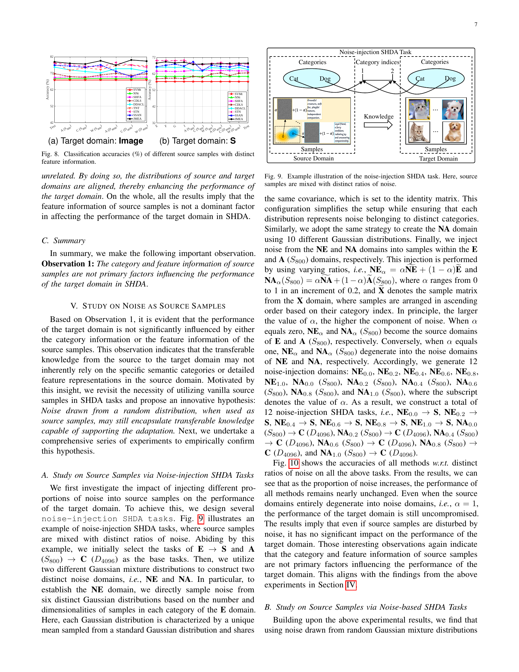
🔼 This figure displays the classification accuracy achieved by various semi-supervised heterogeneous domain adaptation (SHDA) methods across different SHDA tasks. The key aspect highlighted is the performance variation when using source samples with differing feature representations. The goal is to show whether the origin (e.g., text, image, or noise) of the source data significantly impacts the success of knowledge transfer to the target domain. Specifically, it investigates whether the choice of feature representation in the source samples significantly affects the accuracy of SHDA methods on the target domain.
read the caption
Figure 8: Classification accuracies (%) of different source samples with distinct feature information.

🔼 This figure illustrates a noise-injection SHDA task. In a standard SHDA task, the goal is to learn from labeled source data and limited labeled target data to classify unlabeled target data. Here, the source data is augmented by mixing it with different ratios of noise. This allows the researchers to analyze how the introduction of noise into the source data impacts the SHDA model’s ability to classify the unlabeled target data, helping to understand how robust the models are to noisy inputs. The noise is not added directly into the original feature space, but into the representation learned by the network itself.
read the caption
Figure 9: Example illustration of the noise-injection SHDA task. Here, source samples are mixed with distinct ratios of noise.

🔼 The figure shows the classification accuracy for different source samples with distinct feature information. Specifically, it displays the performance of several machine learning methods (SVMt, NNt, SHFA, CDLS, DDACL, TNT, STN, SSAN, JMEA) when using various source domains (Text, A (S800), C (S800), W (S800), A (D4096), C (D4096), W (D4096)) to predict the target domain, which is ‘S’ in this subfigure. The x-axis represents the source domain, and the y-axis represents the classification accuracy. The purpose is to investigate how different feature representations in source samples impact the target prediction accuracy in semi-supervised heterogeneous domain adaptation (SHDA).
read the caption
(a) Target domain: S

🔼 This figure displays the classification accuracy results for different source samples (with distinct feature information) when the target domain is C (D4096). The x-axis represents the different source domains used, showing the performance of several SHDA methods (and two supervised learning baselines) on the target domain’s classification task. It’s part of an empirical study exploring the influence of different types of source samples on SHDA performance. The goal is to determine whether the category or feature information in source samples impacts the target domain’s performance.
read the caption
(b) Target domain: C (D4096subscript𝐷4096D_{4096}italic_D start_POSTSUBSCRIPT 4096 end_POSTSUBSCRIPT)

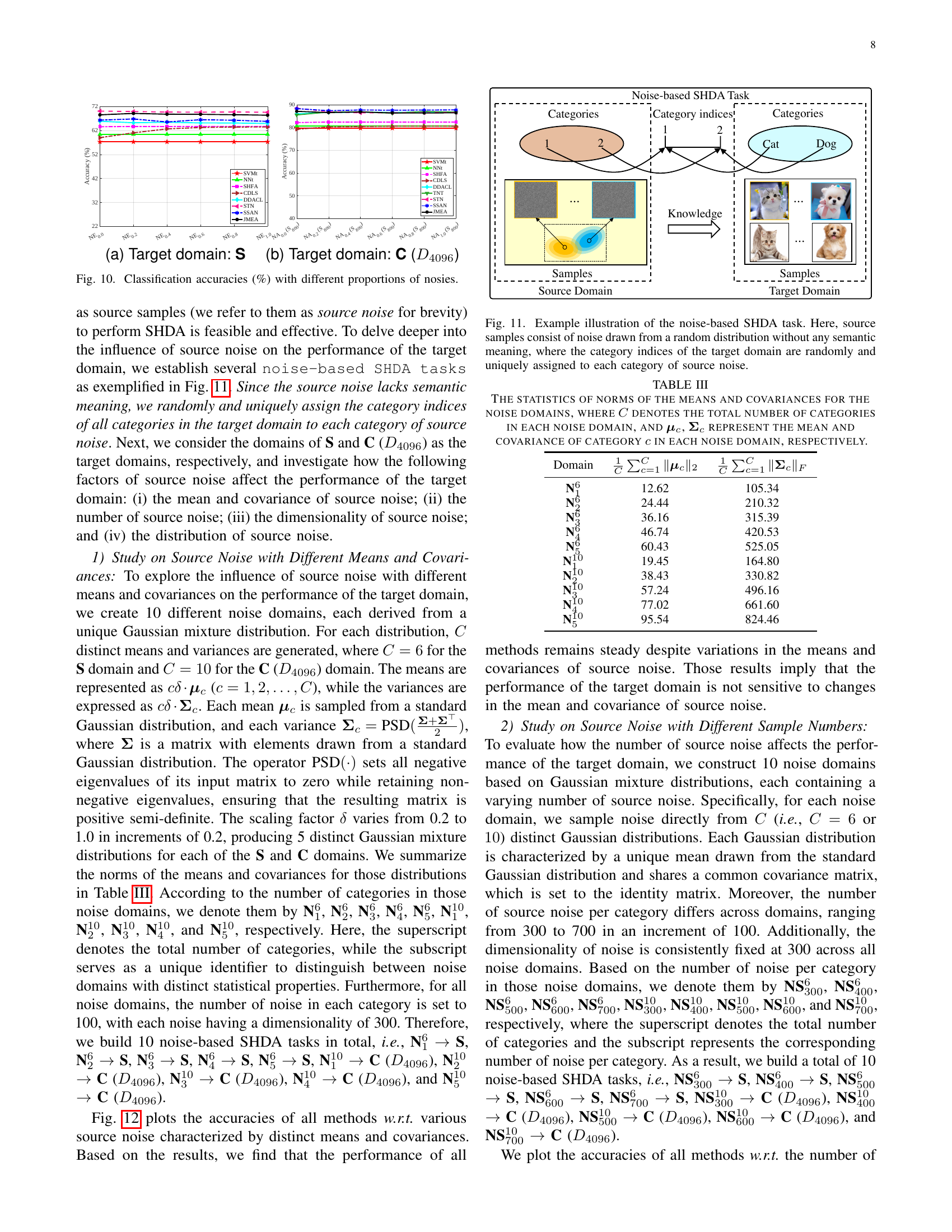
🔼 This figure displays the classification accuracy results obtained from applying various domain adaptation methods to tasks where the source data is increasingly contaminated with noise. The x-axis represents the proportion of noise added to the original source data, ranging from 0% to 100% (in increments of 20%). The y-axis displays the classification accuracy. Two target domains were used: domain S (textual data) and domain C (images). The results illustrate how each method’s performance changes with increasing noise levels, showing its resilience (or lack thereof) to noisy source data in semi-supervised heterogeneous domain adaptation (SHDA).
read the caption
Figure 10: Classification accuracies (%) with different proportions of nosies.

🔼 This figure illustrates a noise-based semi-supervised heterogeneous domain adaptation (SHDA) task. Instead of using actual data as source samples, the source domain consists entirely of noise generated from a random distribution. This noise lacks any semantic meaning or relationship to real-world categories. To connect the noise to the target domain, the category indices (labels) of the target domain are randomly and uniquely mapped to each category of the source noise. This setup is used to investigate whether transferable knowledge can be extracted from purely random data in the context of SHDA.
read the caption
Figure 11: Example illustration of the noise-based SHDA task. Here, source samples consist of noise drawn from a random distribution without any semantic meaning, where the category indices of the target domain are randomly and uniquely assigned to each category of source noise.

🔼 The figure shows the classification accuracy for different methods across various source noise samples with the target domain being the multilingual Reuters dataset (S). It illustrates how the performance of different domain adaptation methods changes as increasing proportions of noise are injected into the source samples. The x-axis represents the increasing proportion of noise, and the y-axis represents the classification accuracy. Each line represents a different domain adaptation method, allowing for comparison of their robustness to noise in the source data.
read the caption
(a) Target domain: S

🔼 This figure shows the classification accuracy results on the target domain C (using 4096-dimensional DeCAF features). The x-axis represents different proportions of noise injected into the source samples, ranging from 0% (no noise) to 100% (pure noise). The y-axis represents the classification accuracy. The plot displays the performance of various SHDA methods under different levels of noise in the source data. This experiment investigates the impact of noise in the source domain on the SHDA performance.
read the caption
(b) Target domain: C (D4096subscript𝐷4096D_{4096}italic_D start_POSTSUBSCRIPT 4096 end_POSTSUBSCRIPT)

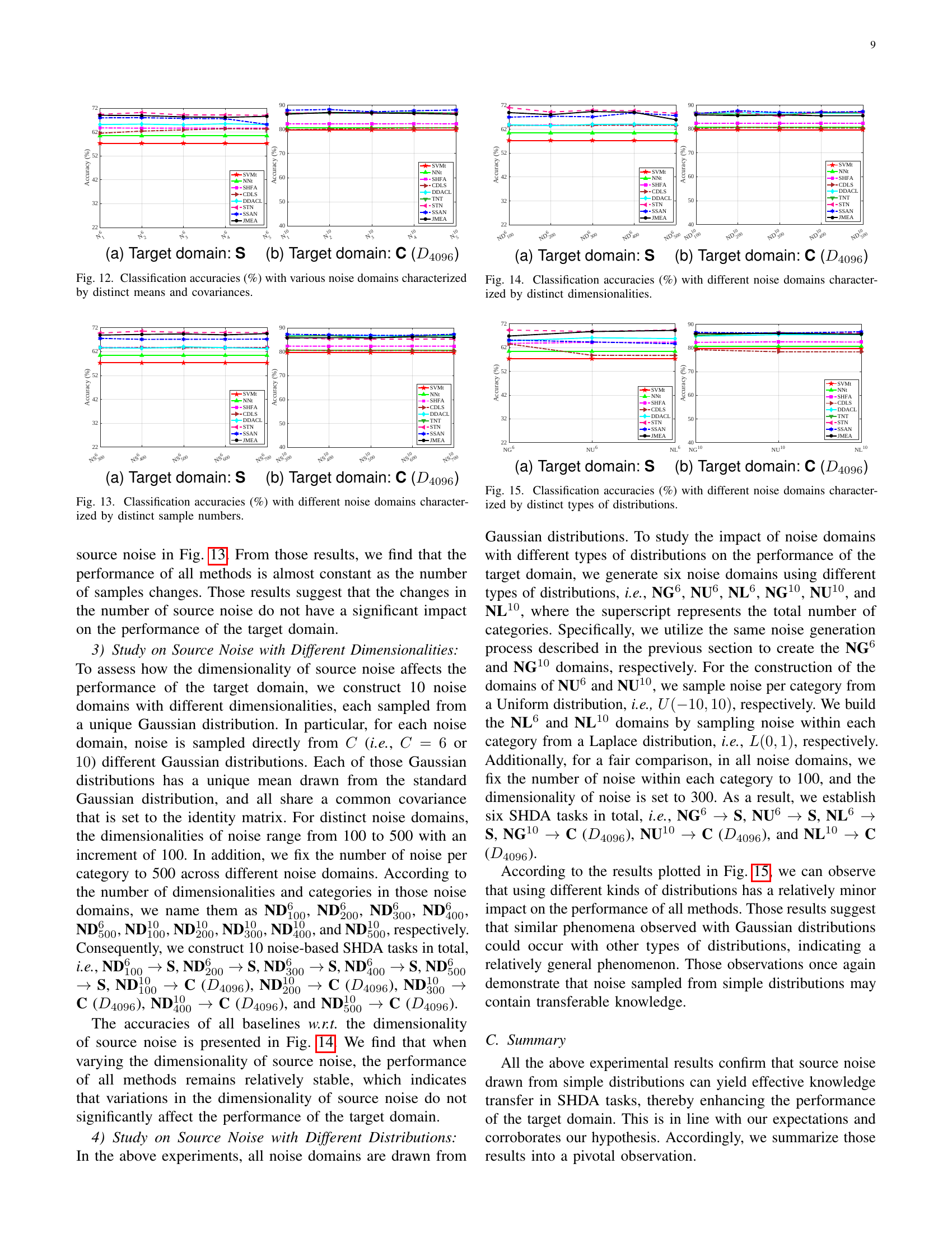
🔼 Figure 12 presents the classification accuracy results for various noise-based semi-supervised heterogeneous domain adaptation (SHDA) tasks. Different noise domains are generated using Gaussian mixture distributions with varying means and covariances. The performance across nine different SHDA methods (and two supervised learning baselines) are shown for two target domains: the ‘S’ domain and the ‘C (D4096)’ domain. The purpose of the experiment is to investigate how the statistical properties of the noise (means and covariances) impact the success of domain adaptation.
read the caption
Figure 12: Classification accuracies (%) with various noise domains characterized by distinct means and covariances.

🔼 This figure shows the classification accuracy for different source samples with distinct feature information. The x-axis represents different source domains (text, A(S800), C(S800), W(S800), A(D4096), C(D4096), W(D4096)), while the y-axis represents the classification accuracy. The plot shows that the accuracy remains relatively stable across different source domains, indicating that the type of source sample may have less impact on the overall performance than other factors, and suggesting that noise may contain transferable knowledge.
read the caption
(a) Target domain: S

🔼 The figure shows the classification accuracy results for different source samples with distinct feature information when the target domain is C (D4096). The x-axis represents different source data types, and the y-axis represents the accuracy. The plot visualizes the performance of different SHDA methods and supervised learning methods (SVMt, NNt) under this condition.
read the caption
(b) Target domain: C (D4096subscript𝐷4096D_{4096}italic_D start_POSTSUBSCRIPT 4096 end_POSTSUBSCRIPT)

🔼 This figure displays the classification accuracy results for several semi-supervised heterogeneous domain adaptation (SHDA) methods. The accuracy is measured using different noise domains where the number of samples in each noise category is varied. The noise samples are used as the source domain in these SHDA experiments. The purpose is to study the impact of the number of noise samples on the performance of the target domain. Different target domains are included in this experiment.
read the caption
Figure 13: Classification accuracies (%) with different noise domains characterized by distinct sample numbers.

🔼 The figure shows the classification accuracy for different source samples with distinct feature information. The x-axis lists various source domains, representing different types of data used (e.g., text, images from different sources). The y-axis displays the classification accuracy on the target domain S. Each bar represents a different SHDA method tested. The plot illustrates the impact of different source data on the performance of SHDA algorithms in terms of classification accuracy on the target domain.
read the caption
(a) Target domain: S

🔼 The figure shows the classification accuracy for different source samples with distinct feature information, specifically focusing on the target domain C (D4096). It demonstrates the performance of various methods (SVMt, NNt, SHFA, CDLS, DDACL, TNT, STN, SSAN, JMEA) when using different source domains (Text, A (S800), C (S800), W (S800), A (D4096), C (D4096), W (D4096)) for semi-supervised heterogeneous domain adaptation (SHDA). The x-axis represents the different source domains, while the y-axis shows the classification accuracy.
read the caption
(b) Target domain: C (D4096subscript𝐷4096D_{4096}italic_D start_POSTSUBSCRIPT 4096 end_POSTSUBSCRIPT)

🔼 This figure displays the classification accuracy results for various machine learning methods across multiple experiments. Each experiment uses a different noise domain as the source of training data. The key difference between the experiments is the dimensionality of the noise data (ranging from 100 to 500). The results illustrate how the performance of the algorithms changes with varying dimensionality of the noise used as training input, and helps to assess the impact of this feature on overall accuracy.
read the caption
Figure 14: Classification accuracies (%) with different noise domains characterized by distinct dimensionalities.

🔼 This figure visualizes the classification accuracies achieved by different methods across various noise-injection SHDA tasks, specifically focusing on the target domain ‘S’. The x-axis represents different proportions of noise injected into the source samples, ranging from 0 to 1. The y-axis displays the classification accuracy. The various lines represent different SHDA methods and supervised learning baselines. The figure demonstrates the robustness of the methods across different levels of noise in the source domain.
read the caption
(a) Target domain: S
🔼 This figure shows the classification accuracy results for different source samples with varying feature information when the target domain is the Caltech-256 dataset represented with 4096-dimensional DeCAF features (D4096). Different source domains are used, and the plot illustrates how the choice of source data affects the performance of the target domain classification task.
read the caption
(b) Target domain: C (D4096subscript𝐷4096D_{4096}italic_D start_POSTSUBSCRIPT 4096 end_POSTSUBSCRIPT)

🔼 Figure 15 displays the results of classification accuracy for various SHDA methods when different types of noise distributions are used as source data. Specifically, six types of noise domains were generated: three with 6 categories (NG6, NU6, NL6) and three with 10 categories (NG10, NU10, NL10). NG denotes noise drawn from Gaussian distributions, NU from uniform distributions, and NL from Laplace distributions. The figure shows how each method’s performance varies across these different noise distributions for two target domains (S and C). This helps analyze the impact of the source noise’s distribution on SHDA performance.
read the caption
Figure 15: Classification accuracies (%) with different noise domains characterized by distinct types of distributions.
🔼 The figure shows the classification accuracies of different supervised learning methods and semi-supervised heterogeneous domain adaptation (SHDA) methods on the target domain S. The x-axis represents different types of source samples, showing that performance is relatively stable regardless of whether source data comes from text, images, or noise. This visualization supports the hypothesis that noise can contain transferable knowledge for SHDA.
read the caption
(a) Target domain: S

🔼 The figure shows the classification accuracy results for various noise-injection SHDA tasks, where the target domain is the ‘S’ domain (Multilingual Reuters Collection dataset). Different methods are compared, and the x-axis represents different ratios of noise added to the source samples. The plot illustrates how the performance of SHDA methods changes as the amount of noise in the source samples increases, showcasing the robustness or sensitivity of the methods to noisy input.
read the caption
(b) Target domain: S

🔼 The figure shows the classification accuracy for different source noise with varying proportions on the target domain C (D4096). The x-axis represents the ratio of noise added to the source data, ranging from 0 to 1. The y-axis shows the classification accuracy. Multiple lines represent different SHDA methods used in the experiment, illustrating the effect of different levels of noise on model performance in a heterogeneous domain adaptation task.
read the caption
(c) Target domain: C (D4096subscript𝐷4096D_{4096}italic_D start_POSTSUBSCRIPT 4096 end_POSTSUBSCRIPT)

🔼 Figure 10(d) presents the classification accuracy results for various noise injection methods on the Caltech-256 dataset (using DeCAF6 features), where source samples contain varying levels of noise from a Gaussian distribution. The x-axis shows the different methods, and the y-axis shows the accuracy. Different colored lines represent different noise levels (from 0% to 100%). The figure demonstrates that even with 100% noise as source data, the SHDA methods achieve comparable performance to those with real source samples, suggesting the surprising conclusion that noise can contain transferable knowledge.
read the caption
(d) Target domain: C (D4096subscript𝐷4096D_{4096}italic_D start_POSTSUBSCRIPT 4096 end_POSTSUBSCRIPT)

🔼 Figure 16 shows the correlation between the discriminability and transferability of the source domain and the performance improvement in the target domain. The discriminability (ℒs) measures how well the source data is separated; lower values indicate better separation. Transferability (ℒs,t) measures how similar the source and target domains are; lower values indicate better transferability. The performance improvement ratio (𝒫r) shows how much better the KTF model performs compared to a standard supervised learning model (NNt). The plots and correlation coefficients demonstrate a strong negative correlation: Better discriminability and transferability in the source domain lead to better performance improvements in the target domain.
read the caption
Figure 16: Correlation between ℒssubscriptℒ𝑠\mathcal{L}_{s}caligraphic_L start_POSTSUBSCRIPT italic_s end_POSTSUBSCRIPT and 𝒫rsubscript𝒫𝑟\mathcal{P}_{r}caligraphic_P start_POSTSUBSCRIPT italic_r end_POSTSUBSCRIPT, as well as between ℒs,tsubscriptℒ𝑠𝑡\mathcal{L}_{s,t}caligraphic_L start_POSTSUBSCRIPT italic_s , italic_t end_POSTSUBSCRIPT and 𝒫rsubscript𝒫𝑟\mathcal{P}_{r}caligraphic_P start_POSTSUBSCRIPT italic_r end_POSTSUBSCRIPT. Here, ℒssubscriptℒ𝑠\mathcal{L}_{s}caligraphic_L start_POSTSUBSCRIPT italic_s end_POSTSUBSCRIPT represents the discriminability of the source domain, ℒs,tsubscriptℒ𝑠𝑡\mathcal{L}_{s,t}caligraphic_L start_POSTSUBSCRIPT italic_s , italic_t end_POSTSUBSCRIPT characterizes the transferability of the source domain, and 𝒫rsubscript𝒫𝑟\mathcal{P}_{r}caligraphic_P start_POSTSUBSCRIPT italic_r end_POSTSUBSCRIPT denotes the performance improvement ratio in the target domain.

🔼 This figure shows a t-SNE visualization of the source and target data distributions for the task of transferring knowledge from a noise-based source domain (N6) to a target domain (S) at iteration 1 (t=1). The ‘+’ symbols represent source samples, ‘x’ symbols represent labeled target samples, and ‘o’ symbols represent unlabeled target samples. Each color corresponds to a different category, illustrating the separation (or lack thereof) of categories in both domains at the start of the adaptation process.
read the caption
(a) N6 →→\rightarrow→ S: t=1𝑡1t=1italic_t = 1

🔼 This figure shows a t-SNE visualization of the data from a semi-supervised heterogeneous domain adaptation (SHDA) experiment. Specifically, it displays the results for the task N6 → S at iteration 200. The plot visualizes the features of source samples (represented by ‘+’), labeled target samples (’*’), and unlabeled target samples (‘o’). Each color corresponds to a distinct category. The figure illustrates how the features of source and target samples are distributed and how well-separated they are in the feature space after 200 iterations of the adaptation process. This is used to analyze the alignment of source and target domains throughout the adaptation process, helping to understand knowledge transfer in SHDA.
read the caption
(b) N6 →→\rightarrow→ S: t=200𝑡200t=200italic_t = 200

🔼 This figure displays a t-distributed stochastic neighbor embedding (t-SNE) visualization of the results from the N6 → S experiment at iteration 400. The visualization shows the separation of source noise samples (marked with ‘+’) and target samples (labeled with ‘x’ and unlabeled with ‘o’). Each color represents a different category. The figure illustrates the degree of separation achieved between source and target categories in the common subspace at this training iteration.
read the caption
(c) N6 →→\rightarrow→ S: t=400𝑡400t=400italic_t = 400

🔼 This t-SNE visualization shows the results of applying the Knowledge Transfer Framework (KTF) to the N6 → S task (source noise with 6 categories mapped to the target domain S) at iteration 600. Each point represents a sample. The ‘+’ symbol denotes a source noise sample; the ‘*’ symbol denotes a labeled target sample; and the ‘o’ symbol denotes an unlabeled target sample. Each color represents a different category. The figure illustrates the clustering and separation of samples in the common subspace learned by the KTF, demonstrating the alignment of source and target domains.
read the caption
(d) N6 →→\rightarrow→ S: t=600𝑡600t=600italic_t = 600

🔼 This figure shows a t-distributed stochastic neighbor embedding (t-SNE) visualization of the source and target data distributions for a specific semi-supervised heterogeneous domain adaptation (SHDA) task. The task involves using a noise-based source domain (N10) with 10 categories to adapt to a target image domain (C(D4096)). The visualization is shown at the very beginning of the adaptation process (t=1). Each point represents a data sample, colored according to its category. The ‘+’ symbol indicates source samples, the ‘*’ symbol indicates labeled target samples, and the ‘o’ symbol indicates unlabeled target samples. This visualization illustrates the initial separation (or lack thereof) of the source and target data points before the adaptation process begins.
read the caption
(e) N10 →→\rightarrow→ C (D4096subscript𝐷4096D_{4096}italic_D start_POSTSUBSCRIPT 4096 end_POSTSUBSCRIPT): t=1𝑡1t=1italic_t = 1

🔼 This figure shows a t-SNE visualization of the features of source and target samples for the task N10 -> C(D4096) at iteration 200. The plus sign (+) represents source noise samples, while the circles (o) and squares (■) denote unlabeled and labeled target samples, respectively. Each color corresponds to a different category. The visualization demonstrates how the separation of the target sample categories improves as the model trains. This is a visualization to show discriminability and transferability.
read the caption
(f) N10 →→\rightarrow→ C (D4096subscript𝐷4096D_{4096}italic_D start_POSTSUBSCRIPT 4096 end_POSTSUBSCRIPT): t=200𝑡200t=200italic_t = 200

🔼 This figure shows a t-SNE visualization of the results for the task where source samples consist of noise (N10) and the target domain is C (D4096). The visualization is at time step t=400, showing the separation of different categories in the target domain. The ‘+’ symbols represent source samples (noise), while ‘●’ indicates labeled target samples, and ‘o’ represents unlabeled target samples. Each color represents a different category.
read the caption
(g) N10 →→\rightarrow→ C (D4096subscript𝐷4096D_{4096}italic_D start_POSTSUBSCRIPT 4096 end_POSTSUBSCRIPT): t=400𝑡400t=400italic_t = 400

🔼 This figure shows the t-distributed stochastic neighbor embedding (t-SNE) visualization of the N10 → C(D4096) task at iteration 600. The plus signs (+) represent source samples (noise), the asterisks (*) denote labeled target samples, and the circles (o) represent unlabeled target samples. Each color corresponds to a different category. The visualization demonstrates the separation of categories in the common subspace achieved by the model, highlighting the alignment of source and target data distributions.
read the caption
(h) N10 →→\rightarrow→ C (D4096subscript𝐷4096D_{4096}italic_D start_POSTSUBSCRIPT 4096 end_POSTSUBSCRIPT): t=600𝑡600t=600italic_t = 600

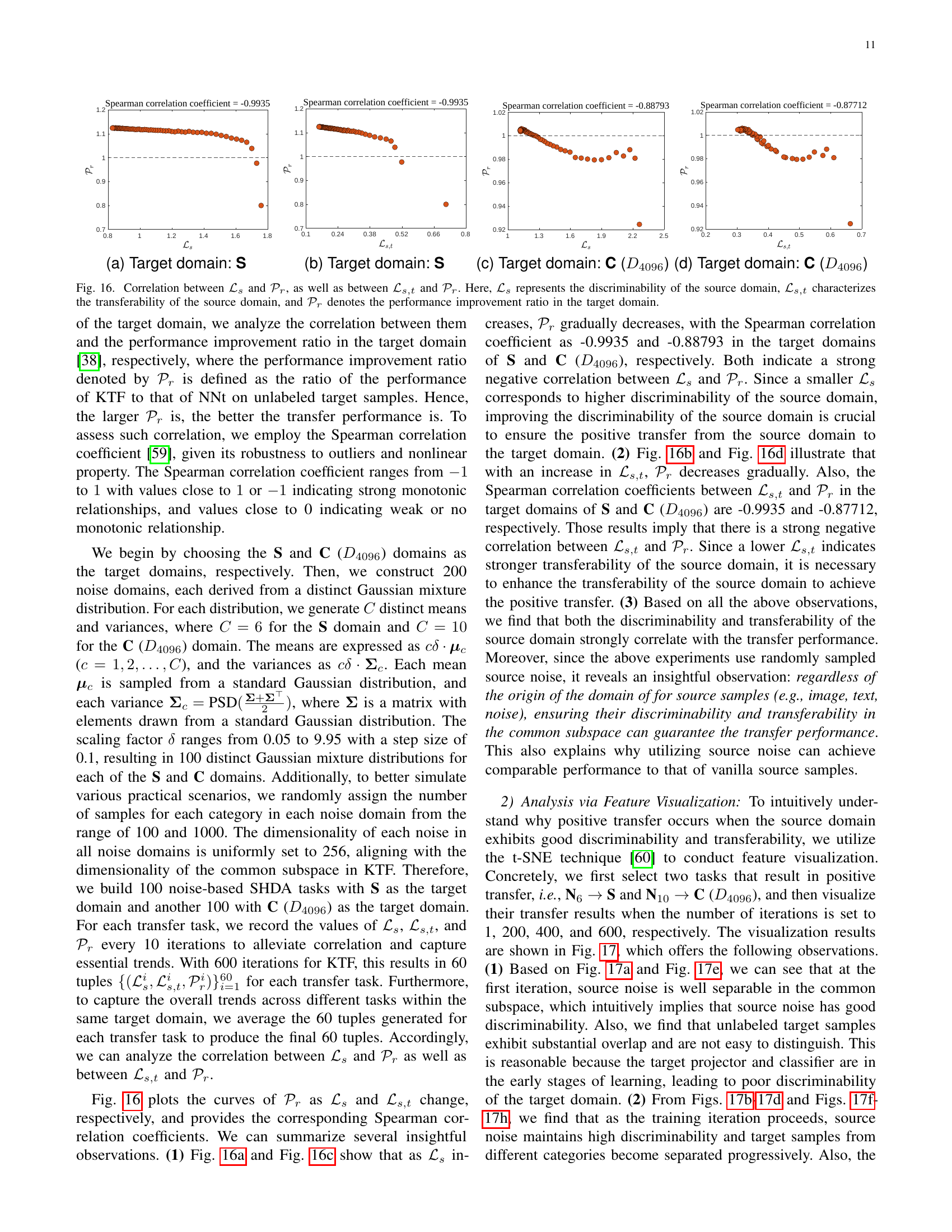
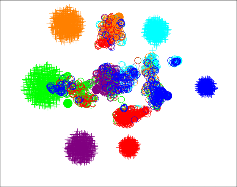
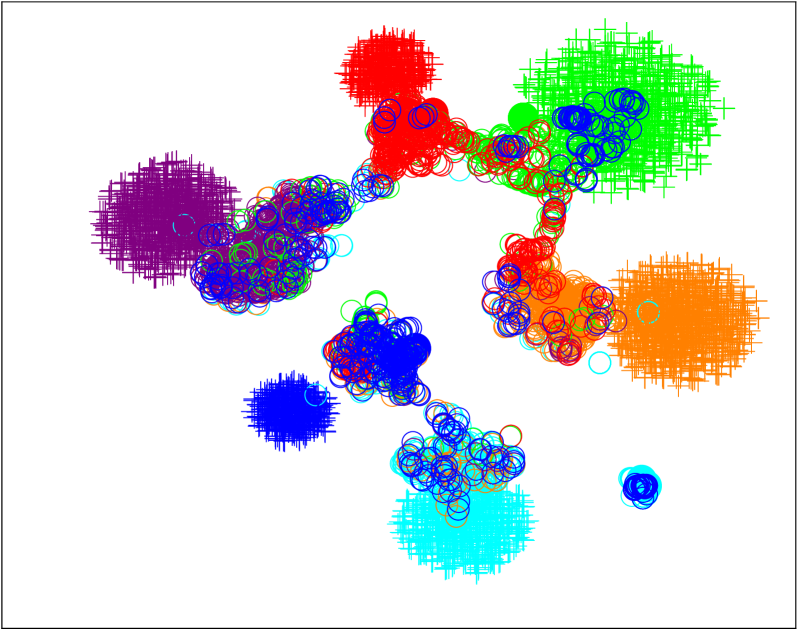
🔼 This figure visualizes the results of t-SNE dimensionality reduction applied to source and target data in two semi-supervised heterogeneous domain adaptation (SHDA) tasks: N6→S and N10→C(D4096). Different shapes represent different data types: ‘+’ for source samples, ‘∙’ for labeled target samples, and ‘∘’ for unlabeled target samples. Each color represents a distinct category. The four columns for each task show the data points at different iteration numbers (t), demonstrating how the data clusters evolve as the SHDA algorithm proceeds. This visualization helps illustrate the gradual alignment of source and target data distributions during the adaptation process, highlighting the discriminability of the source domain and the increasing separability of target samples as iterations progress.
read the caption
Figure 17: t-SNE visualization on the tasks of N6 →→\rightarrow→ S and N10 →→\rightarrow→ C (D4096subscript𝐷4096D_{4096}italic_D start_POSTSUBSCRIPT 4096 end_POSTSUBSCRIPT). Here, the ‘+’ sign denotes a source sample, the ‘∙∙\bullet∙’ sign represents a labeled target sample, and the ‘∘\circ∘’ sign stands for an unlabeled target sample. Each color corresponds to a distinct category, and t𝑡titalic_t is the current number of iterations.

🔼 This figure displays a t-distributed stochastic neighbor embedding (t-SNE) visualization of the results from a noise-based semi-supervised heterogeneous domain adaptation (SHDA) task. Specifically, it shows the feature distribution of source noise (represented by ‘+’), labeled target samples (’*’), and unlabeled target samples (‘o’) at the beginning of the training process (iteration 1). Each color represents a different category. The figure is part of an analysis investigating the transferability of knowledge from noise to target samples, revealing how noise samples separate by category in the common subspace.
read the caption
(a) N6 →→\rightarrow→ S: t = 1

🔼 This figure shows the t-SNE visualization of the transfer process on the task of N6 –> S (Noise with 6 categories as source domain to the S target domain) at iteration 200. The ‘+’ sign represents source samples, the ‘*’ sign represents labeled target samples, and the ‘o’ sign represents unlabeled target samples. Each color represents a distinct category. The plot visualizes how the source and target samples are distributed in the common subspace, and how their distributions change as the training progresses. The visualization helps to understand how the knowledge from the source domain is transferred to the target domain during the domain adaptation process.
read the caption
(b) N6 →→\rightarrow→ S: t = 200

🔼 This figure shows a t-SNE visualization of the results from a semi-supervised heterogeneous domain adaptation (SHDA) task where the source domain is noise (N6) and the target domain is the Reuters dataset (S). The visualization is shown at iteration 400 of the training process. Each point represents a sample and the color indicates the true class label of the sample. The visualization demonstrates the gradual alignment of the distributions of the source and target domains as training progresses. This alignment is important because it shows the positive transfer of knowledge from the source noise to the target dataset.
read the caption
(c) N6 →→\rightarrow→ S: t = 400

🔼 This t-SNE visualization shows the results of the N6 → S task in the study on transferable knowledge in SHDA. The image displays the distribution of source noise (represented by ‘+’), labeled target samples (’*’), and unlabeled target samples (‘o’) in the common subspace at iteration 600. Each color represents a different category. The visualization aims to illustrate the alignment between the source and target domains, demonstrating how the discriminability of the source noise is transferred to the target samples as the transferability of the source domain improves.
read the caption
(d) N6 →→\rightarrow→ S: t = 600
More on tables
| Method | Type | URL for Code | Publication |
|---|---|---|---|
| SVMt [33] | Supervised Learning | https://www.csie.ntu.edu.tw/~cjlin/libsvm/ | ACM TIST 2011 |
| NNt [34] | Supervised Learning | https://github.com/tensorflow/tensorflow | OSDI 2016 |
| SHFA [35] | Shallow Projection SHDA | https://github.com/wenli-vision/SHFA_release | TPAMI 2014 |
| CDLS [36] | Shallow Projection SHDA | https://github.com/yaohungt/Cross-Domain-Landmarks-Selection-CDLS-/tree/master | CVPR 2016 |
| DDACL [27] | Shallow Projection SHDA | https://github.com/yyyaoyuan/DDA | Pattern Recognition 2020 |
| TNT [37] | Deep Projection SHDA | https://github.com/wyharveychen/TransferNeuralTrees | ECCV 2016 |
| STN [24] | Deep Projection SHDA | https://github.com/yyyaoyuan/STN | ACM MM 2019 |
| SSAN [29] | Deep Projection SHDA | https://github.com/BIT-DA/SSAN | ACM MM 2020 |
| JMEA [25] | Deep Projection SHDA | https://github.com/fang-zhen/Semi-supervised-Heterogeneous-Domain-Adaptation | TPAMI 2023 |
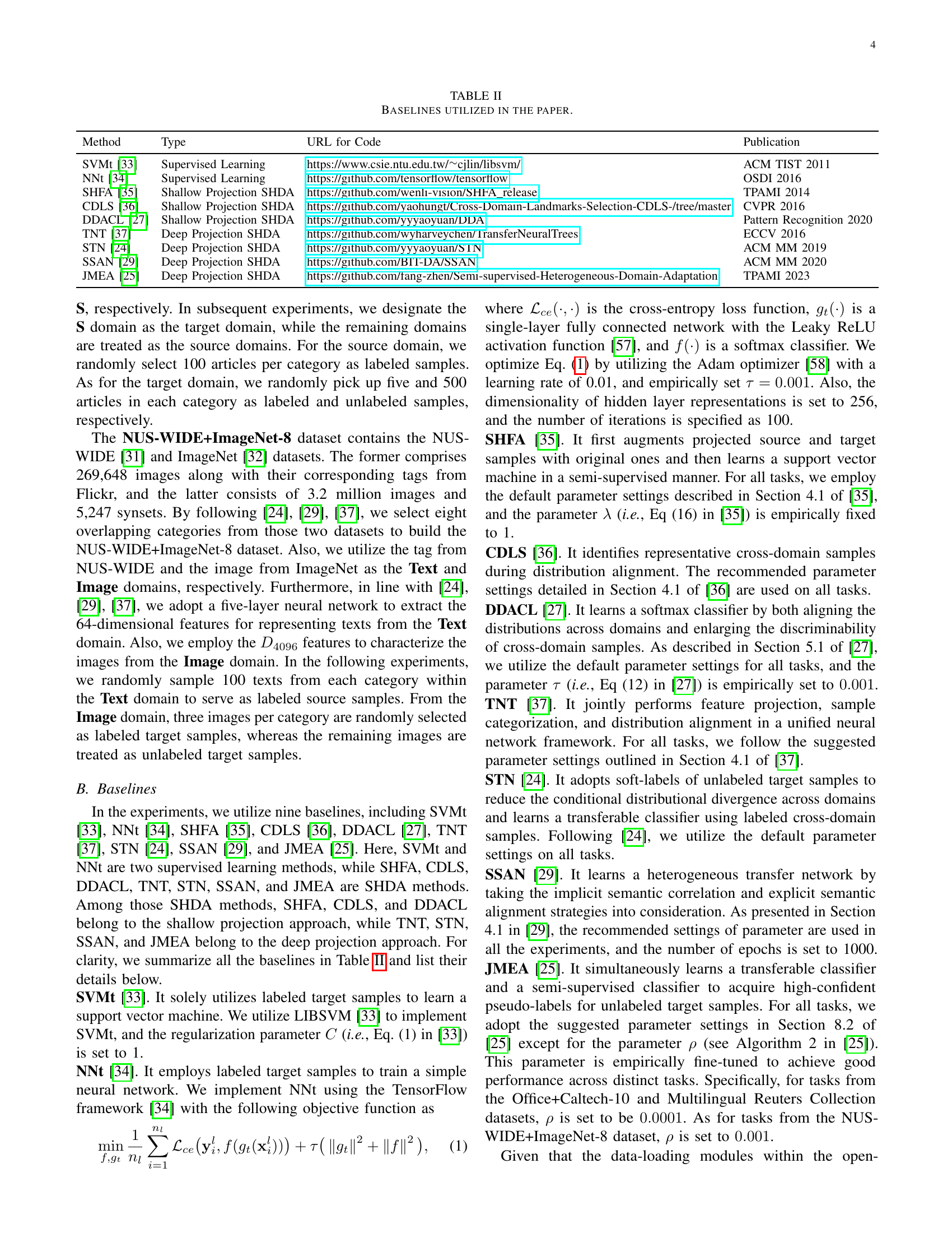
🔼 Table II lists the nine baseline methods used in the paper’s experiments for comparison. It includes two supervised learning methods (SVMt and NNt) and seven semi-supervised heterogeneous domain adaptation (SHDA) methods (SHFA, CDLS, DDACL, TNT, STN, SSAN, and JMEA). For each method, the table provides the method’s type (supervised learning or SHDA), a short description, and a URL to the source code.
read the caption
TABLE II: Baselines utilized in the paper.
| Domain | ||
|---|---|---|
| N | 12.62 | 105.34 |
| N | 24.44 | 210.32 |
| N | 36.16 | 315.39 |
| N | 46.74 | 420.53 |
| N | 60.43 | 525.05 |
| N | 19.45 | 164.80 |
| N | 38.43 | 330.82 |
| N | 57.24 | 496.16 |
| N | 77.02 | 661.60 |
| N | 95.54 | 824.46 |
🔼 Table III presents the statistical measures for various noise domains generated using Gaussian mixture distributions. Specifically, it shows the norms (magnitude) of the mean vectors (𝝁c) and covariance matrices (𝚺c) for each category (c) within each noise domain. The table helps in understanding the variability and distribution characteristics of the different noise datasets used in the experiments.
read the caption
TABLE III: The statistics of norms of the means and covariances for the noise domains, where C𝐶Citalic_C denotes the total number of categories in each noise domain, and 𝝁csubscript𝝁𝑐\bm{\mu}_{c}bold_italic_μ start_POSTSUBSCRIPT italic_c end_POSTSUBSCRIPT, 𝚺csubscript𝚺𝑐\bm{\Sigma}_{c}bold_Σ start_POSTSUBSCRIPT italic_c end_POSTSUBSCRIPT represent the mean and covariance of category c𝑐citalic_c in each noise domain, respectively.
Full paper#