Discovering highly efficient low-weight quantum error-correcting codes with reinforcement learning

2502.14372

Austin Yubo He et el.

🤗 2025-02-21

TL;DR
#

Quantum error correction is vital for fault-tolerant quantum computing, yet high measurement weight increases error. Quantum low-density parity-check (qLDPC) codes, focus on asymptotic properties, but finite-size optimization lags. Traditional methods like greedy algorithms struggle to achieve needed distances. Weight reduction, lowering check weight while maintaining code properties increases physical qubit overhead.

This paper introduces a versatile, computationally efficient method for stabilizer code weight reduction using reinforcement learning (RL). This method produces new low-weight codes that outperform current state-of-the-art results, drastically reducing physical qubit overhead. The RL framework offers insights into code parameter interplay and demonstrates how RL can advance quantum code discovery, which paves the way for practical quantum technologies.

Key Takeaways
#

Why does it matter?
#

This research offers a versatile RL framework for optimizing quantum error-correcting codes, potentially transforming fault-tolerant quantum computing. It surpasses existing weight reduction methods and opens avenues for exploring coding strategies, making it crucial for quantum tech.

Visual Insights
#

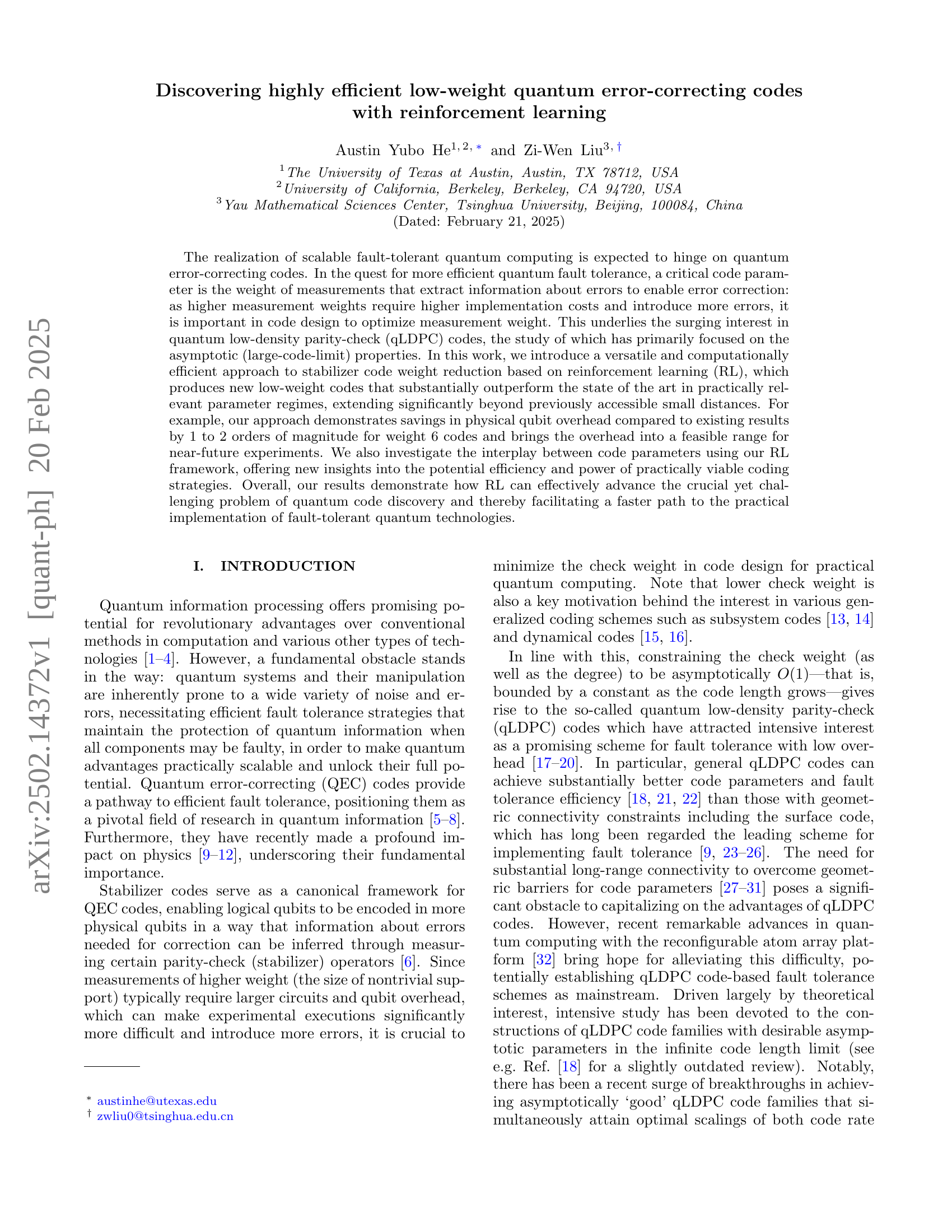
🔼 This figure illustrates the reinforcement learning (RL) framework used to discover highly efficient low-weight quantum error-correcting codes. The RL agent interacts with an environment representing a Tanner graph, which is a graphical representation of the quantum code. At each step, the agent decides whether to add or remove an edge in the graph (the action). The environment then updates the graph based on the agent’s action and returns a reward. This reward is calculated using the code’s new distance and weight. The reward signal informs the agent about the effectiveness of its actions, guiding the learning process towards better code designs (i.e., codes with smaller weights and larger distances).
read the caption
Figure 1: An illustration of our RL scheme. The RL agent (left) maintains a policy network that, given the state of the Tanner graph, selects an action of adding or removing an edge. The environment (right) updates the graph accordingly and returns a reward based on the code’s new distance and weight. This reward signal is then used to update the policy network, guiding the agent toward better code designs.

Base Code	Hastings [44]	Sabo et al. [46]	RL(6,3)
$[\![45,9,3]\!]_{\!(8,3)}$	$[\![2892,9,5]\!]_{\!(6,6)}$	$[\![65,9,4]\!]_{\!(6,3)}$	$[\![45,9,3]\!]_{\!(6,3)}$
$[\![74,4,4]\!]_{\!(6,4)}$	$[\![7466,4,6]\!]_{\!(6,8)}$	$[\![100,4,4]\!]_{\!(6,3)}$	$[\![74,4,4]\!]_{\!(6,3)}$
$[\![65,9,4]\!]_{\!(8,3)}$	$[\![6844,9,5]\!]_{\!(6,8)}$	$[\![89,9,4]\!]_{\!(6,3)}$	$[\![65,9,4]\!]_{\!(6,3)}$
$[\![58,16,3]\!]_{\!(8,3)}$	$[\![5085,16,3]\!]_{\!(6,8)}$	$[\![136,16,4]\!]_{\!(6,3)}$	$[\![58,16,3]\!]_{\!(6,3)}$

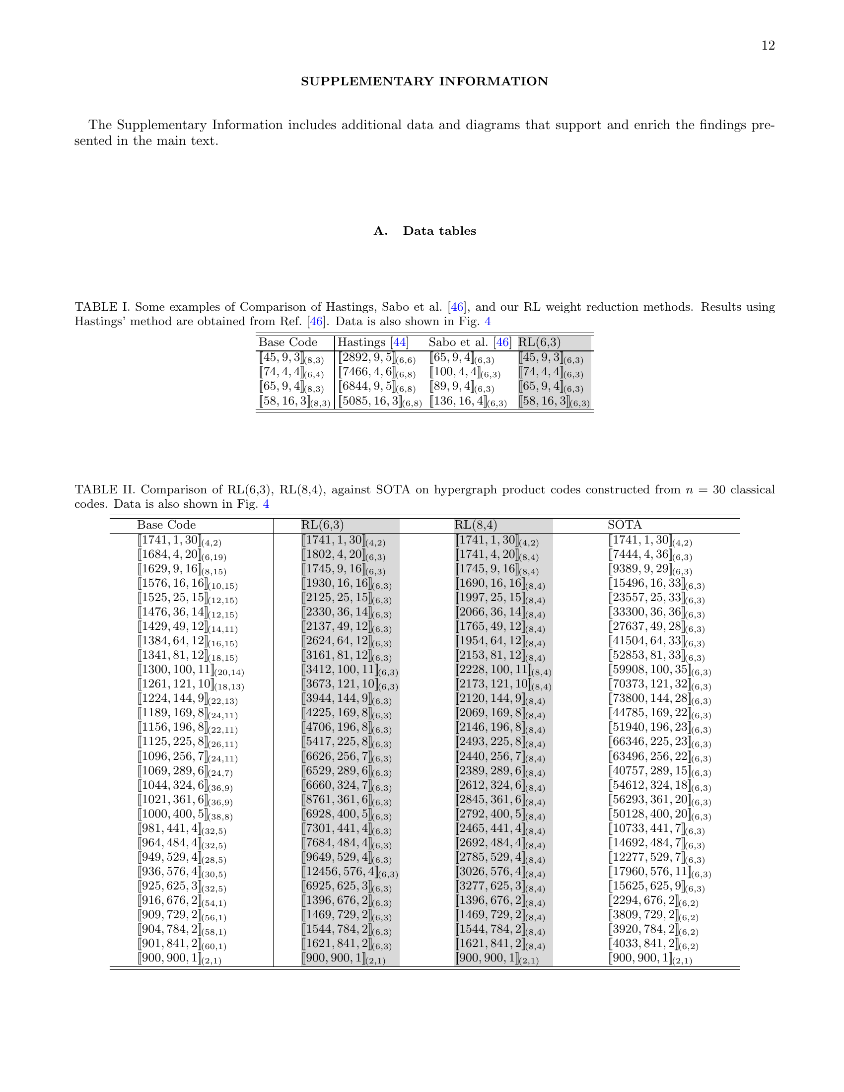
🔼 This table compares the performance of three different weight reduction methods for quantum error-correcting codes: the method by Hastings, the method by Sabo et al. [46], and the reinforcement learning (RL) method proposed in this paper. For several example quantum codes, it shows the number of physical qubits required by each method to achieve a specific weight reduction. The data illustrates the significant reduction in physical qubit overhead achieved by the RL method compared to the previous methods.
read the caption
Table 1: Some examples of Comparison of Hastings, Sabo et al. [46], and our RL weight reduction methods. Results using Hastings’ method are obtained from Ref. [46]. Data is also shown in Fig. 4

In-depth insights
#

RL for QEC Codes
#

Reinforcement learning (RL) holds promise for quantum error correction (QEC). Traditional code design is complex, but RL offers a data-driven approach. RL can explore vast code spaces, potentially finding novel codes beyond human intuition. RL excels at optimizing code parameters like distance and threshold. RL trains an agent to iteratively improve codes based on reward signals, such as minimizing logical error rate. There are few challenges such as choosing the right reward function and model architecture. This field is rapidly growing with new applications.

Finite-Size Limits
#

In the realm of quantum error correction, finite-size limits pose a significant hurdle. While theoretical constructs often focus on asymptotic behavior (large code limits), practical quantum computers operate with a finite number of qubits. This necessitates a shift in focus towards optimizing code parameters within realistic, finite-size regimes. The performance of quantum error-correcting codes drastically differs when moving from idealized, asymptotic scenarios to the constraints of real-world quantum devices. Achieving optimal weight reduction in stabilizer codes is challenging but crucial for practical implementation, as higher measurement weights can introduce errors and increase circuit complexity. Finite code lengths also impact the effectiveness of decoding algorithms. Sophisticated approximation methods may be needed, or the codes could exhibit high logical failure rates.

Weight Reduction
#

Weight reduction in quantum error correction is a crucial optimization strategy to minimize the physical qubit overhead, as higher weight measurements increase implementation costs and error rates. Methods like Hastings’ aim for asymptotic reductions, while others target finite-size regimes. The approach is to decrease check weight while maintaining code properties, balancing node degree reduction with distance preservation. This leads to robust error correction, with reward functions guiding reinforcement learning. Masking enforces constraints, restricting agents to target weights, and enhancing learning. RL is used to find lower weight codes, improving code parameters, by creating new codes and modifying code parameters, which addresses the difficulty of learning large qLDPC codes.

Hypergraph Product
#

Hypergraph product codes represent a significant advancement in constructing quantum error-correcting codes (QECCs) by leveraging classical codes, offering a pathway to create quantum low-density parity-check (qLDPC) codes with desirable properties. By cleverly combining parity-check matrices of classical codes, they enable the creation of CSS codes, ensuring orthogonality and therefore validity. Their appeal lies in the potential to achieve favorable code parameters and fault-tolerance, making them a central object of study in the pursuit of practical and efficient QECCs. The product structure facilitates theoretical analysis and allows for the construction of codes with well-defined properties. This structure also guides the application of reinforcement learning framework to refine and optimize them. Optimizing codes is done in terms of weight and degree, as explored within the research paper. These optimized codes are a promising direction for realizing fault-tolerant quantum computation.

Megaquop Scaling
#

While not explicitly a section in this paper, “Megaquop Scaling” evokes the challenge of achieving quantum error correction (QEC) at the scale of millions of physical qubits (megaquops), a scale believed necessary for fault-tolerant quantum computation beyond toy problems. This paper implicitly addresses this by focusing on reducing qubit overhead through reinforcement learning (RL) designed quantum codes, given that achieving this scale requires minimizing the resources required per logical qubit. The paper emphasizes finite size regimes, this is critical to achieve the near-term megaquop scaling in early quantum devices. Specifically, the RL framework effectively uncovers codes with far more reduced overhead than previous analytical schemes, getting the devices closer to practical implementation. Code distances are now higher and logical qubits now scale higher, implying reduced resources needed for reliable computation.

More visual insights
#

More on figures

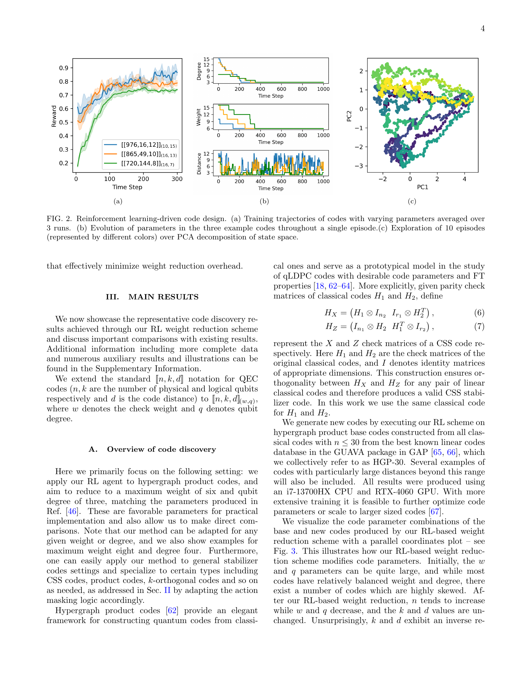
🔼 This figure displays the training trajectories of three different codes with varying parameters, averaged over three runs. It showcases how the reward (a measure of the code’s quality) changes over time steps during the reinforcement learning process. The parameters used to generate each code are given in the legend: e.g., [976,16,12] represents the values of the parameters (n, k, d)(w, q).
read the caption
(a)

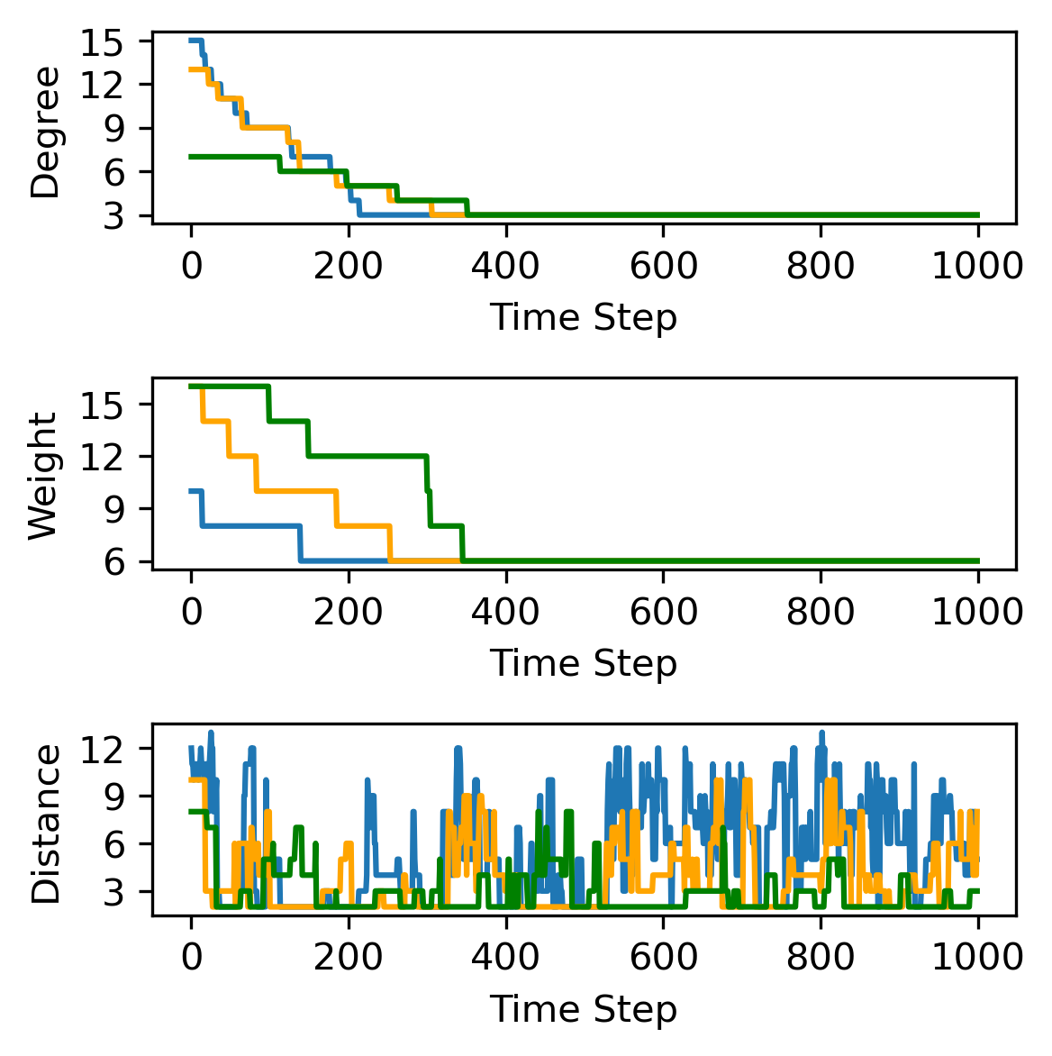
🔼 This figure (Figure 2b) shows the evolution of code parameters (weight, degree, and distance) over a single training episode of the reinforcement learning algorithm for weight reduction. It illustrates how the RL agent modifies these parameters to optimize code properties. Specifically, it demonstrates the interplay between weight/degree reduction and distance preservation during the learning process. The curves illustrate the dynamic adjustments to the code’s characteristics to achieve better code parameters.
read the caption
(b)

🔼 This figure shows the exploration of the RL agent in the state space of Tanner graphs over 10 episodes. Each color represents a different episode. The plot uses Principal Component Analysis (PCA) to reduce the dimensionality of the high-dimensional Tanner graph state space to two principal components (PC1 and PC2). The trajectory of each episode in this reduced space shows how the agent explores different graph structures while learning to optimize the code parameters.
read the caption
(c)

🔼 This figure shows the results of using reinforcement learning to design quantum error-correcting codes. Panel (a) displays the learning curves for three different code designs, illustrating how the reward (a measure of code quality) changes over time. Panel (b) zooms in on a single learning episode for those same three codes, showing the evolution of key code parameters (weight, degree, and distance) as the algorithm iteratively improves the design. Finally, Panel (c) provides a dimensionality-reduced view of the state space explored by the algorithm across 10 different learning episodes, offering insights into the search process and the variety of code designs discovered.
read the caption
Figure 2: Reinforcement learning-driven code design. (a) Training trajectories of codes with varying parameters averaged over 3 runs. (b) Evolution of parameters in the three example codes throughout a single episode.(c) Exploration of 10 episodes (represented by different colors) over PCA decomposition of state space.

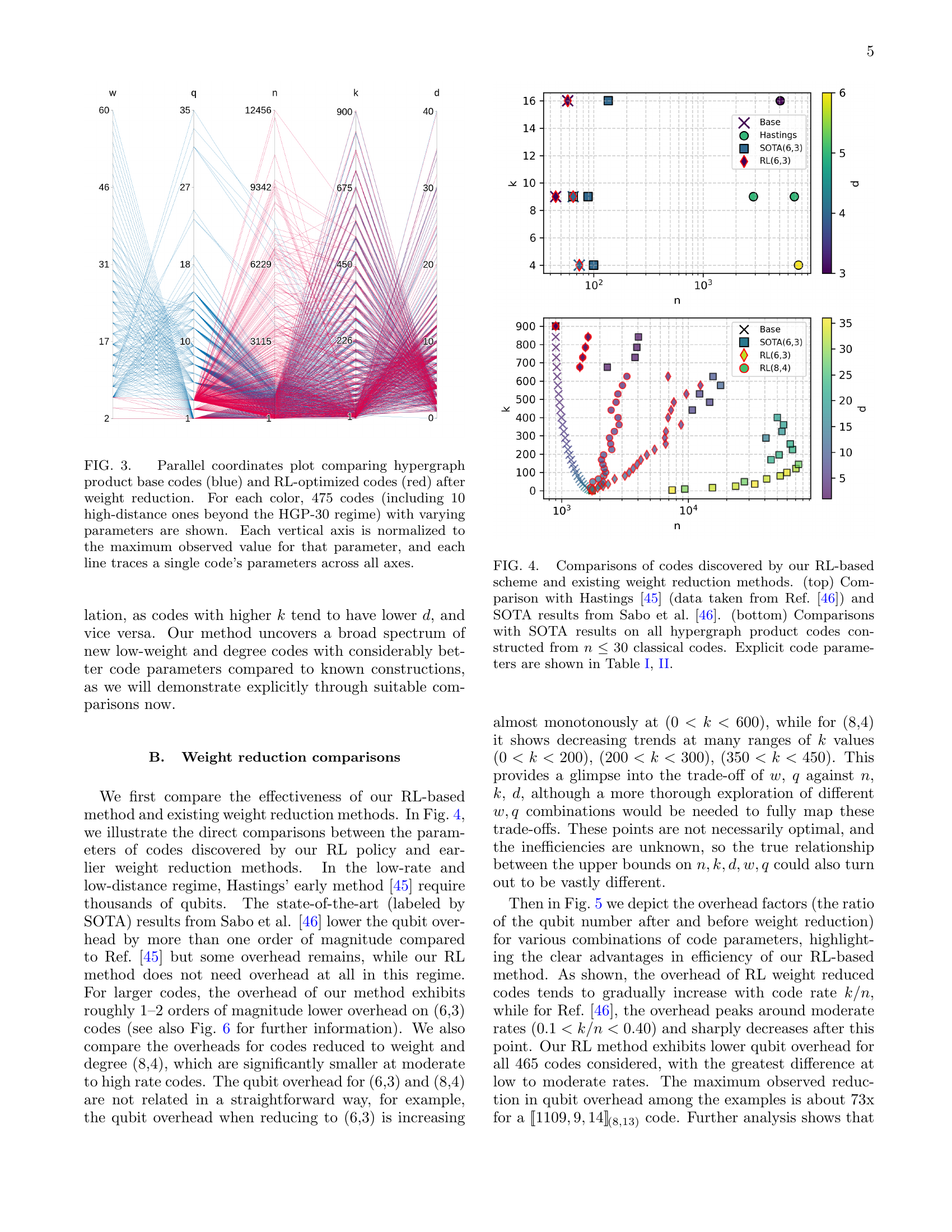
🔼 Figure 3 visualizes the effect of the reinforcement learning (RL)-based weight reduction method on hypergraph product codes. It uses a parallel coordinates plot to compare the parameters of original hypergraph product codes (blue lines) and the codes after RL optimization (red lines). The plot includes 475 codes of each type, with the additional 10 high-distance codes extending beyond the HGP-30 dataset. Each vertical axis represents a code parameter (n, k, d, w, q), normalized to its maximum observed value. Each line in the plot shows a single code’s parameter values across all axes, providing a visual comparison of the parameter distributions before and after weight reduction.
read the caption
Figure 3: Parallel coordinates plot comparing hypergraph product base codes (blue) and RL-optimized codes (red) after weight reduction. For each color, 475 codes (including 10 high-distance ones beyond the HGP-30 regime) with varying parameters are shown. Each vertical axis is normalized to the maximum observed value for that parameter, and each line traces a single code’s parameters across all axes.

🔼 Figure 4 presents a comparison of the performance of the reinforcement learning (RL)-based weight reduction method introduced in the paper against two other existing methods: Hastings’ method and the state-of-the-art (SOTA) method from Sabo et al. The top part of the figure focuses on comparisons for low-rate, low-distance codes, directly contrasting the qubit overhead of each method. The bottom part expands the comparison to a wider range of hypergraph product codes with various parameters constructed using classical codes (n≤30). The explicit code parameters are tabulated in Tables I and II in the supplementary information.
read the caption
Figure 4: Comparisons of codes discovered by our RL-based scheme and existing weight reduction methods. (top) Comparison with Hastings [45] (data taken from Ref. [46]) and SOTA results from Sabo et al. [46]. (bottom) Comparisons with SOTA results on all hypergraph product codes constructed from n≤30𝑛30n\leq 30italic_n ≤ 30 classical codes. Explicit code parameters are shown in Table 1, 2.

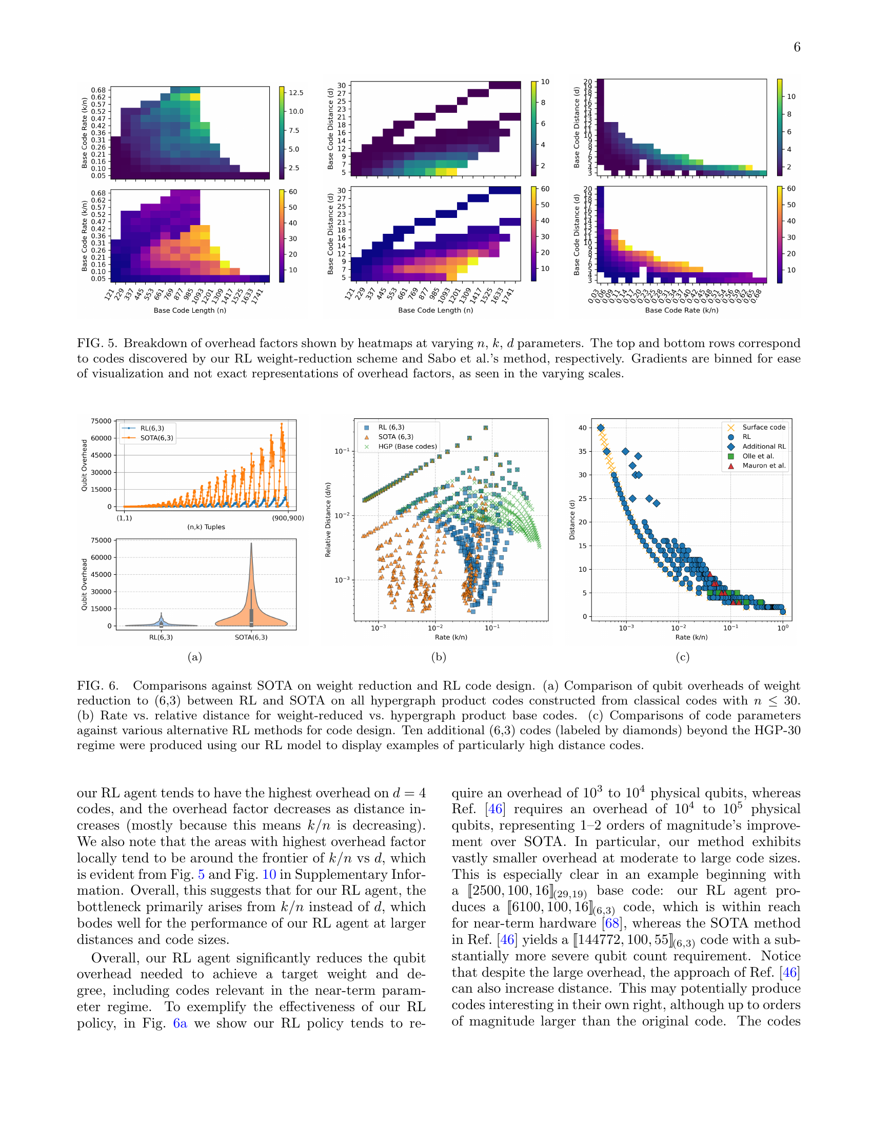
🔼 Figure 5 presents a comparison of the overhead factors achieved by two different weight-reduction methods: the reinforcement learning (RL) approach introduced in this paper and the method proposed by Sabo et al. The overhead factor is calculated as the ratio of physical qubits used after the weight reduction process to the number of physical qubits used before the process. The figure displays heatmaps showing the distribution of these overhead factors for different values of code parameters, namely the code length (n), the number of logical qubits (k), and the code distance (d). Separate heatmaps are presented for both methods. The color gradient in each heatmap represents the magnitude of the overhead factor. Note that the color scales differ between the heatmaps, and the color gradients are binned for better visualization, resulting in approximate rather than precise values.
read the caption
Figure 5: Breakdown of overhead factors shown by heatmaps at varying n𝑛nitalic_n, k𝑘kitalic_k, d𝑑ditalic_d parameters. The top and bottom rows correspond to codes discovered by our RL weight-reduction scheme and Sabo et al.’s method, respectively. Gradients are binned for ease of visualization and not exact representations of overhead factors, as seen in the varying scales.

🔼 This figure displays the evolution of the spectral gap and eigenvalues of the Tanner graphs over time steps during training. The spectral gap, representing the difference between the first two largest eigenvalues, starts high and decreases as training progresses. This indicates a change in the structure of the Tanner graphs, moving from well-structured expanders to less structured ones. Simultaneously, the eigenvalues that were originally concentrated near +1 and -1 spread out, further highlighting the structural changes. The observations suggest that the RL agent is discovering codes outside the typical theoretical frameworks relying on expansion properties, even if this sacrifices performance in message-passing-based decoding.
read the caption
(a)

🔼 This figure displays the evolution of various parameters during a single training episode of the reinforcement learning model. The plots track the changes in distance, weight, and degree of the Tanner graph representing the quantum code over time. This illustrates the learning process and how the RL agent modifies the code’s properties to reduce its weight while aiming to maintain or improve the distance. The fluctuations in the parameters reveal the search strategy of the RL agent, balancing exploration and exploitation.
read the caption
(b)

🔼 This figure shows the exploration of the RL agent in the state space of Tanner graphs over 10 episodes. Each color represents a different episode. The graph displays the principle components (PC1 and PC2) of the state space. The exploration shows how the agent modifies the Tanner graph, which represents the stabilizer code, over the course of the training process.
read the caption
(c)

🔼 Figure 6 presents a comparison of the performance of the proposed reinforcement learning (RL)-based weight reduction method against existing state-of-the-art (SOTA) techniques. Subfigure (a) shows a direct comparison of qubit overhead for codes reduced to weight 6 and degree 3, highlighting the significant reduction achieved by the RL method. Subfigure (b) illustrates the relationship between code rate and relative distance for both weight-reduced codes and the original hypergraph product base codes. Subfigure (c) compares the code parameters (n, k, d) obtained using the RL approach to those generated by alternative RL-based code design methods. Notably, the RL method discovers several new codes with exceptionally high distances, which are represented by diamonds in the plot, exceeding the capabilities of previously reported methods.
read the caption
Figure 6: Comparisons against SOTA on weight reduction and RL code design. (a) Comparison of qubit overheads of weight reduction to (6,3) between RL and SOTA on all hypergraph product codes constructed from classical codes with n≤30𝑛30n\leq 30italic_n ≤ 30. (b) Rate vs. relative distance for weight-reduced vs. hypergraph product base codes. (c) Comparisons of code parameters against various alternative RL methods for code design. Ten additional (6,3) codes (labeled by diamonds) beyond the HGP-30 regime were produced using our RL model to display examples of particularly high distance codes.

🔼 The figure shows training trajectories of three different codes with varying parameters, averaged over three runs. Each line represents a single training episode. The reward increases as the training progresses and the RL agent finds better code designs. This indicates that the RL model is effectively learning to find better designs. The figure also includes a plot showing the evolution of parameters (weight, degree, and distance) for each example code throughout a single episode, demonstrating a reduction of weight and degree with a corresponding increase in distance.
read the caption
(a)

🔼 This figure (Fig. 2b) displays the evolution of three key parameters—weight, degree, and distance—over a single training episode for three example codes. It visually demonstrates how these parameters change as the reinforcement learning agent modifies the code’s Tanner graph. The plot illustrates the agent’s learning process, showing the interplay between weight reduction, degree control, and distance maintenance, a core challenge in quantum code design. By observing these trends, one can better understand the algorithm’s dynamics and its effectiveness in achieving low-weight, high-distance quantum error-correcting codes.
read the caption
(b)

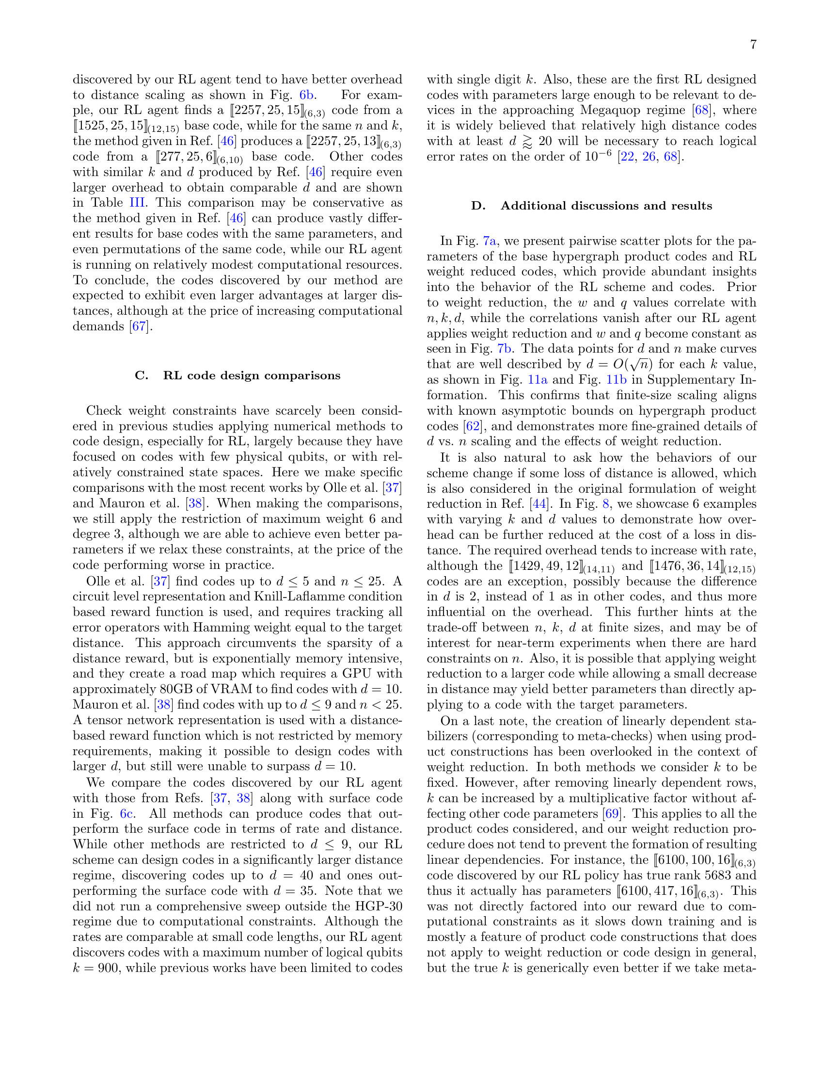
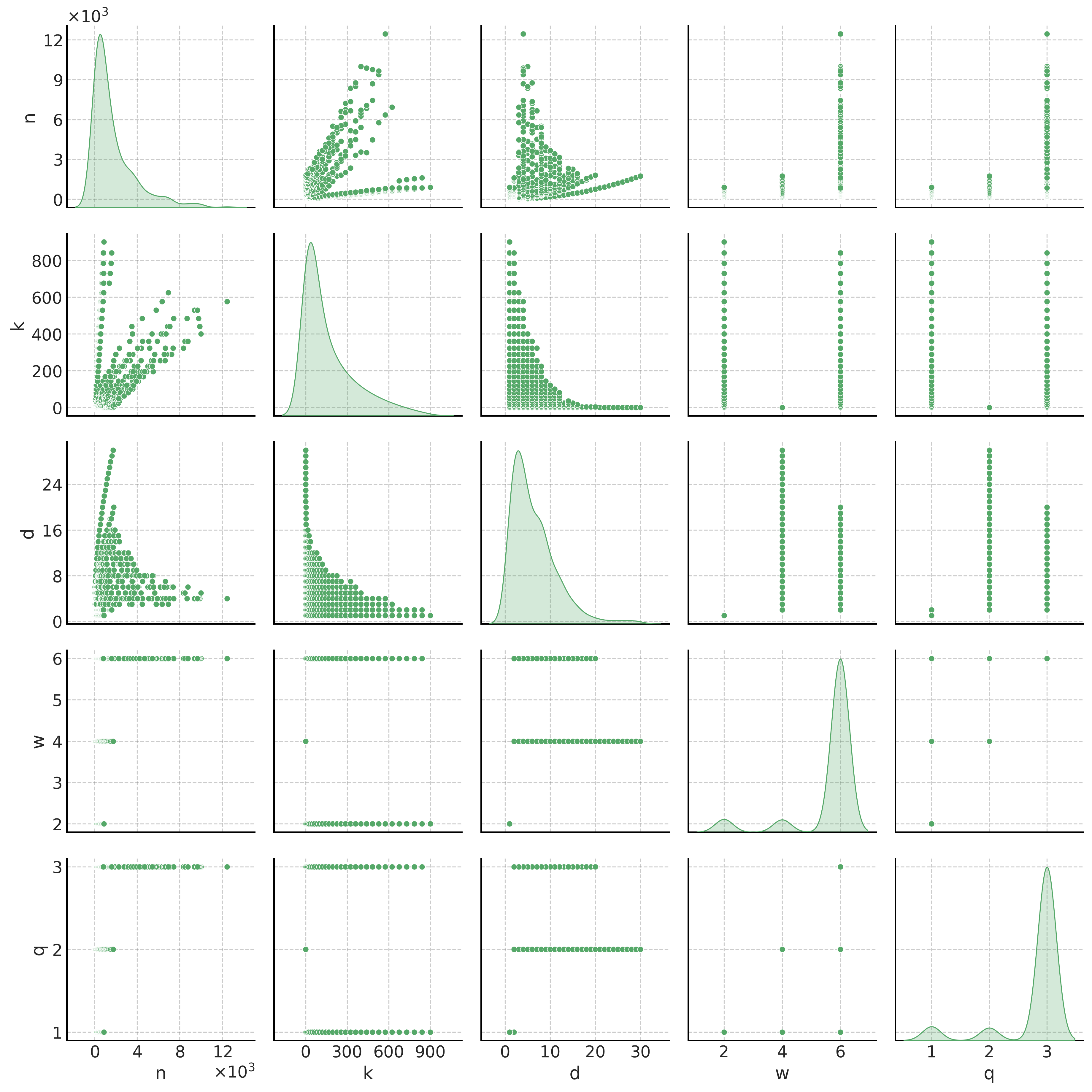
🔼 This figure presents pairwise scatter plots visualizing the relationships between different code parameters before and after applying the reinforcement learning (RL)-based weight reduction technique. Panel (a) shows the distribution of parameters (n: code length, k: number of logical qubits, d: distance, w: check weight, q: qubit degree) in the original hypergraph product codes (HGP-30). Panel (b) displays the same parameters after the RL-based weight reduction algorithm has been applied. Each off-diagonal subplot shows a scatter plot illustrating the correlation (or lack thereof) between a pair of parameters. The diagonal subplots present the individual distributions of each parameter. The plots provide insights into how RL alters the relationship between code parameters during the optimization process, showing both the initial characteristics of the HGP-30 codes and the resulting distribution of parameters after RL optimization.
read the caption
Figure 7: Pairwise scatter plots for the parameters of the HGP-30 base codes and RL codes. (a) Hypergraph product code with parameters n,k,d,w,q𝑛𝑘𝑑𝑤𝑞n,k,d,w,qitalic_n , italic_k , italic_d , italic_w , italic_q before weight reduction, (b) RL codes after weight reduction. Each subplot compares two parameters (off-diagonal) while the diagonal entries depict individual parameter distributions.

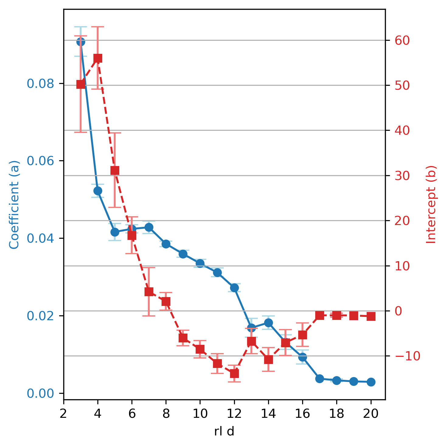
🔼 This figure shows how allowing a small reduction in the code distance (d) can significantly reduce the total number of physical qubits needed. Each bar represents a specific code with its original distance and the overhead incurred when reducing the weight to (6,3) while permitting distance to decrease by 1,2 or 3. The reduction in overhead is substantial in many cases, highlighting the trade-off between code distance and qubit resource requirements. Specific code parameters are detailed in Table 4.
read the caption
Figure 8: Minimum qubit overheads under relaxed distance constraints. Permitting the distance d𝑑ditalic_d to decrease can reduce the total qubit overhead. Code parameters are shown in Table 4

🔼 This figure shows the training trajectories of three example codes with varying parameters, averaged over three runs. The plot illustrates how the reward, which balances node degree reduction with distance preservation, changes over time steps during the training process. It also depicts the evolution of key parameters (distance, weight, and degree) within a single training episode and shows the exploration of the state space of the Tanner graphs over 10 episodes using a PCA decomposition. This visualization helps understand the RL agent’s learning process in optimizing QEC codes.
read the caption
(a)

🔼 This figure (b) shows the evolution of code parameters (weight, degree, and distance) over a single training episode for three example codes. It illustrates how the reinforcement learning agent modifies the code’s structure during the learning process. The x-axis represents time steps in the training process, and the y-axis shows the values of the parameters. Each line corresponds to a specific code parameter.
read the caption
(b)

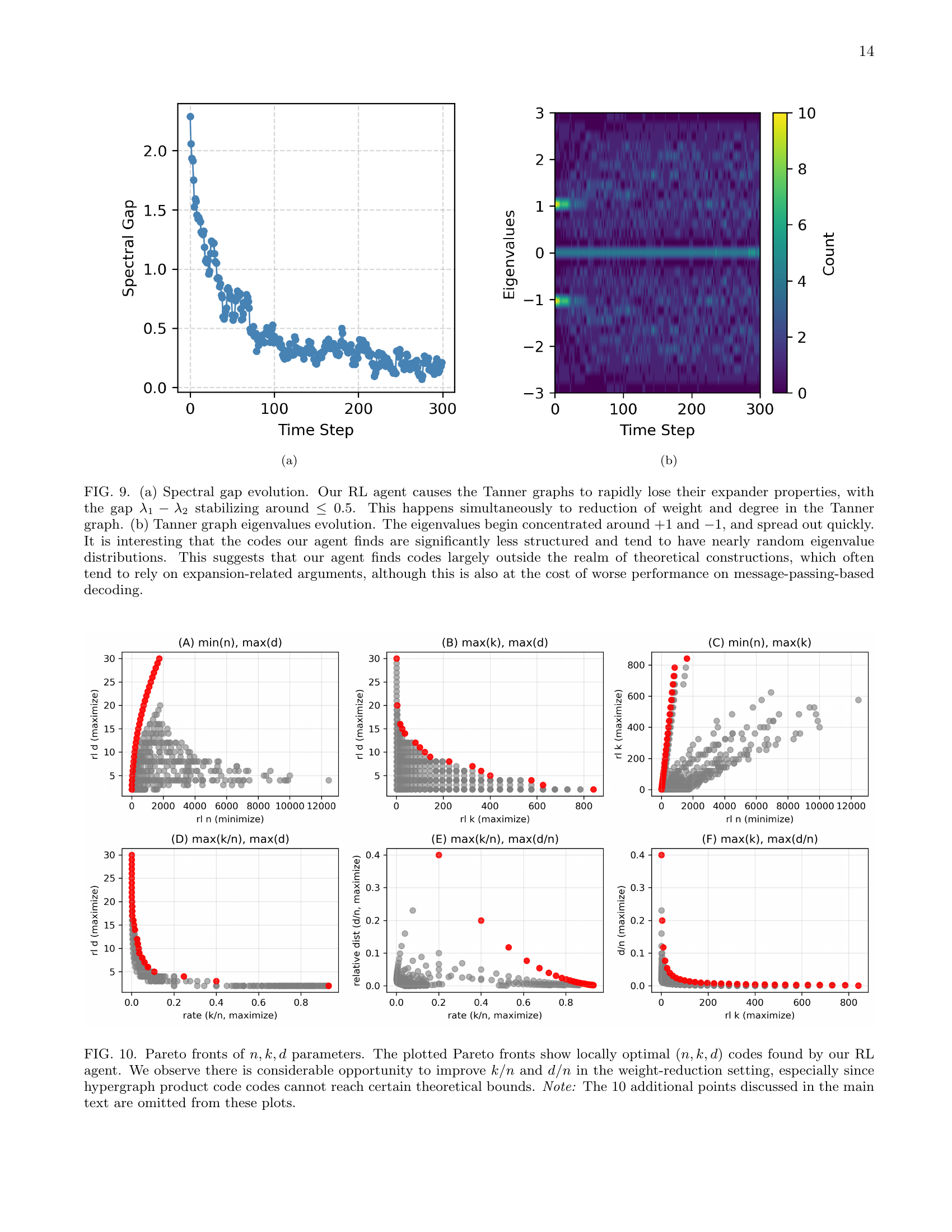
🔼 Figure 9 demonstrates the impact of the reinforcement learning (RL) agent on the spectral properties of Tanner graphs representing quantum error-correcting codes. Panel (a) shows that the spectral gap (the difference between the largest and second largest eigenvalues) decreases and stabilizes below 0.5. This indicates a loss of expander properties, signifying the codes produced by the RL agent are less structured and not easily classifiable using traditional theoretical methods. Panel (b) displays the evolution of eigenvalues over time, starting from being concentrated around +1 and -1 and spreading out. This confirms that the agent generates codes with nearly random eigenvalue distributions, distinct from the structured codes commonly found in theoretical studies that rely on expansion properties. While this unstructured nature implies suboptimal performance with message-passing decoding, the RL algorithm finds codes that are surprisingly efficient for practical implementations.
read the caption
Figure 9: (a) Spectral gap evolution. Our RL agent causes the Tanner graphs to rapidly lose their expander properties, with the gap λ1−λ2subscript𝜆1subscript𝜆2\lambda_{1}-\lambda_{2}italic_λ start_POSTSUBSCRIPT 1 end_POSTSUBSCRIPT - italic_λ start_POSTSUBSCRIPT 2 end_POSTSUBSCRIPT stabilizing around ≤0.5absent0.5\leq 0.5≤ 0.5. This happens simultaneously to reduction of weight and degree in the Tanner graph. (b) Tanner graph eigenvalues evolution. The eigenvalues begin concentrated around +11+1+ 1 and −11-1- 1, and spread out quickly. It is interesting that the codes our agent finds are significantly less structured and tend to have nearly random eigenvalue distributions. This suggests that our agent finds codes largely outside the realm of theoretical constructions, which often tend to rely on expansion-related arguments, although this is also at the cost of worse performance on message-passing-based decoding.

🔼 Figure 10 presents Pareto fronts, which are plots illustrating the trade-off between different parameters of quantum error-correcting codes. Each point on a Pareto front represents a code with specific values for the number of physical qubits (n), the number of logical qubits (k), and the code distance (d). The points are chosen such that no other code exists that is better in terms of all three parameters (i.e., has a higher k and d for the same n or the same k and d with a smaller n). The figure shows Pareto fronts generated by the reinforcement learning (RL) algorithm developed by the authors. The analysis reveals a significant opportunity to optimize the code rate (k/n) and relative distance (d/n) further through their weight reduction technique, surpassing what hypergraph product codes can achieve theoretically.
read the caption
Figure 10: Pareto fronts of n,k,d𝑛𝑘𝑑n,k,ditalic_n , italic_k , italic_d parameters. The plotted Pareto fronts show locally optimal (n,k,d)𝑛𝑘𝑑(n,k,d)( italic_n , italic_k , italic_d ) codes found by our RL agent. We observe there is considerable opportunity to improve k/n𝑘𝑛k/nitalic_k / italic_n and d/n𝑑𝑛d/nitalic_d / italic_n in the weight-reduction setting, especially since hypergraph product code codes cannot reach certain theoretical bounds. Note: The 10 additional points discussed in the main text are omitted from these plots.

🔼 This figure shows the training trajectories of three different codes with varying parameters, averaged over three runs. It demonstrates how the reward, a measure of the code’s quality, changes over time steps during the training process. The evolution of the code’s parameters (distance, weight, degree) is shown throughout a single episode for each code. The exploration of the state space (Tanner graphs) is visualized over ten episodes using a PCA decomposition, showing the range of code designs the RL algorithm explored.
read the caption
(a)

More on tables

Base Code	RL(6,3)	RL(8,4)	SOTA
$[\![1741,1,30]\!]_{\!(4,2)}$	$[\![1741,1,30]\!]_{\!(4,2)}$	$[\![1741,1,30]\!]_{\!(4,2)}$	$[\![1741,1,30]\!]_{\!(4,2)}$
$[\![1684,4,20]\!]_{\!(6,19)}$	$[\![1802,4,20]\!]_{\!(6,3)}$	$[\![1741,4,20]\!]_{\!(8,4)}$	$[\![7444,4,36]\!]_{\!(6,3)}$
$[\![1629,9,16]\!]_{\!(8,15)}$	$[\![1745,9,16]\!]_{\!(6,3)}$	$[\![1745,9,16]\!]_{\!(8,4)}$	$[\![9389,9,29]\!]_{\!(6,3)}$
$[\![1576,16,16]\!]_{\!(10,15)}$	$[\![1930,16,16]\!]_{\!(6,3)}$	$[\![1690,16,16]\!]_{\!(8,4)}$	$[\![15496,16,33]\!]_{\!(6,3)}$
$[\![1525,25,15]\!]_{\!(12,15)}$	$[\![2125,25,15]\!]_{\!(6,3)}$	$[\![1997,25,15]\!]_{\!(8,4)}$	$[\![23557,25,33]\!]_{\!(6,3)}$
$[\![1476,36,14]\!]_{\!(12,15)}$	$[\![2330,36,14]\!]_{\!(6,3)}$	$[\![2066,36,14]\!]_{\!(8,4)}$	$[\![33300,36,36]\!]_{\!(6,3)}$
$[\![1429,49,12]\!]_{\!(14,11)}$	$[\![2137,49,12]\!]_{\!(6,3)}$	$[\![1765,49,12]\!]_{\!(8,4)}$	$[\![27637,49,28]\!]_{\!(6,3)}$
$[\![1384,64,12]\!]_{\!(16,15)}$	$[\![2624,64,12]\!]_{\!(6,3)}$	$[\![1954,64,12]\!]_{\!(8,4)}$	$[\![41504,64,33]\!]_{\!(6,3)}$
$[\![1341,81,12]\!]_{\!(18,15)}$	$[\![3161,81,12]\!]_{\!(6,3)}$	$[\![2153,81,12]\!]_{\!(8,4)}$	$[\![52853,81,33]\!]_{\!(6,3)}$
$[\![1300,100,11]\!]_{\!(20,14)}$	$[\![3412,100,11]\!]_{\!(6,3)}$	$[\![2228,100,11]\!]_{\!(8,4)}$	$[\![59908,100,35]\!]_{\!(6,3)}$
$[\![1261,121,10]\!]_{\!(18,13)}$	$[\![3673,121,10]\!]_{\!(6,3)}$	$[\![2173,121,10]\!]_{\!(8,4)}$	$[\![70373,121,32]\!]_{\!(6,3)}$
$[\![1224,144,9]\!]_{\!(22,13)}$	$[\![3944,144,9]\!]_{\!(6,3)}$	$[\![2120,144,9]\!]_{\!(8,4)}$	$[\![73800,144,28]\!]_{\!(6,3)}$
$[\![1189,169,8]\!]_{\!(24,11)}$	$[\![4225,169,8]\!]_{\!(6,3)}$	$[\![2069,169,8]\!]_{\!(8,4)}$	$[\![44785,169,22]\!]_{\!(6,3)}$
$[\![1156,196,8]\!]_{\!(22,11)}$	$[\![4706,196,8]\!]_{\!(6,3)}$	$[\![2146,196,8]\!]_{\!(8,4)}$	$[\![51940,196,23]\!]_{\!(6,3)}$
$[\![1125,225,8]\!]_{\!(26,11)}$	$[\![5417,225,8]\!]_{\!(6,3)}$	$[\![2493,225,8]\!]_{\!(8,4)}$	$[\![66346,225,23]\!]_{\!(6,3)}$
$[\![1096,256,7]\!]_{\!(24,11)}$	$[\![6626,256,7]\!]_{\!(6,3)}$	$[\![2440,256,7]\!]_{\!(8,4)}$	$[\![63496,256,22]\!]_{\!(6,3)}$
$[\![1069,289,6]\!]_{\!(24,7)}$	$[\![6529,289,6]\!]_{\!(6,3)}$	$[\![2389,289,6]\!]_{\!(8,4)}$	$[\![40757,289,15]\!]_{\!(6,3)}$
$[\![1044,324,6]\!]_{\!(36,9)}$	$[\![6660,324,7]\!]_{\!(6,3)}$	$[\![2612,324,6]\!]_{\!(8,4)}$	$[\![54612,324,18]\!]_{\!(6,3)}$
$[\![1021,361,6]\!]_{\!(36,9)}$	$[\![8761,361,6]\!]_{\!(6,3)}$	$[\![2845,361,6]\!]_{\!(8,4)}$	$[\![56293,361,20]\!]_{\!(6,3)}$
$[\![1000,400,5]\!]_{\!(38,8)}$	$[\![6928,400,5]\!]_{\!(6,3)}$	$[\![2792,400,5]\!]_{\!(8,4)}$	$[\![50128,400,20]\!]_{\!(6,3)}$
$[\![981,441,4]\!]_{\!(32,5)}$	$[\![7301,441,4]\!]_{\!(6,3)}$	$[\![2465,441,4]\!]_{\!(8,4)}$	$[\![10733,441,7]\!]_{\!(6,3)}$
$[\![964,484,4]\!]_{\!(32,5)}$	$[\![7684,484,4]\!]_{\!(6,3)}$	$[\![2692,484,4]\!]_{\!(8,4)}$	$[\![14692,484,7]\!]_{\!(6,3)}$
$[\![949,529,4]\!]_{\!(28,5)}$	$[\![9649,529,4]\!]_{\!(6,3)}$	$[\![2785,529,4]\!]_{\!(8,4)}$	$[\![12277,529,7]\!]_{\!(6,3)}$
$[\![936,576,4]\!]_{\!(30,5)}$	$[\![12456,576,4]\!]_{\!(6,3)}$	$[\![3026,576,4]\!]_{\!(8,4)}$	$[\![17960,576,11]\!]_{\!(6,3)}$
$[\![925,625,3]\!]_{\!(32,5)}$	$[\![6925,625,3]\!]_{\!(6,3)}$	$[\![3277,625,3]\!]_{\!(8,4)}$	$[\![15625,625,9]\!]_{\!(6,3)}$
$[\![916,676,2]\!]_{\!(54,1)}$	$[\![1396,676,2]\!]_{\!(6,3)}$	$[\![1396,676,2]\!]_{\!(8,4)}$	$[\![2294,676,2]\!]_{\!(6,2)}$
$[\![909,729,2]\!]_{\!(56,1)}$	$[\![1469,729,2]\!]_{\!(6,3)}$	$[\![1469,729,2]\!]_{\!(8,4)}$	$[\![3809,729,2]\!]_{\!(6,2)}$
$[\![904,784,2]\!]_{\!(58,1)}$	$[\![1544,784,2]\!]_{\!(6,3)}$	$[\![1544,784,2]\!]_{\!(8,4)}$	$[\![3920,784,2]\!]_{\!(6,2)}$
$[\![901,841,2]\!]_{\!(60,1)}$	$[\![1621,841,2]\!]_{\!(6,3)}$	$[\![1621,841,2]\!]_{\!(8,4)}$	$[\![4033,841,2]\!]_{\!(6,2)}$
$[\![900,900,1]\!]_{\!(2,1)}$	$[\![900,900,1]\!]_{\!(2,1)}$	$[\![900,900,1]\!]_{\!(2,1)}$	$[\![900,900,1]\!]_{\!(2,1)}$

🔼 This table compares the performance of the reinforcement learning (RL) algorithm for weight reduction, specifically the RL(6,3) and RL(8,4) models, against the state-of-the-art (SOTA) method. It focuses on hypergraph product codes constructed from classical codes with a code length (n) of 30. The table presents the parameters of several codes (n,k,d) and their corresponding weights (w) and qubit degrees (q). The parameters illustrate the improved efficiency of the RL-based weight reduction in terms of the physical qubit overhead required to achieve a target code weight and degree.
read the caption
Table 2: Comparison of RL(6,3), RL(8,4), against SOTA on hypergraph product codes constructed from n=30𝑛30n=30italic_n = 30 classical codes. Data is also shown in Fig. 4

Reduced Code

Base Code

RL(6,3)

[\![2257,25,15]\!]_{\!(6,3)}

[\![1525,25,15]\!]_{\!(12,15)}

Sabo et al. [46]

[\![2257,25,13]\!]_{\!(6,3)}

[\![3457,25,15]\!]_{\!(6,3)}

[\![4337,25,17]\!]_{\!(6,3)}

[\![4153,25,16]\!]_{\!(6,3)}

[\![4337,25,16]\!]_{\!(6,3)}

[\![4525,25,17]\!]_{\!(6,3)}

[\![277,25,6]\!]_{\!(6,10)}

[\![325,25,7]\!]_{\!(12,7)}

[\![377,25,9]\!]_{\!(12,7)}

[\![433,25,8]\!]_{\!(10,7)}

[\![493,25,8]\!]_{\!(10,7)}

[\![557,25,8]\!]_{\!(10,7)}

🔼 This table compares the performance of the reinforcement learning (RL)-based weight reduction method against the state-of-the-art (SOTA) method from Sabo et al. [46] for generating quantum error correction codes. It presents several examples, showing for each example the parameters ([n, k, d](w, q)) of the base code used, the parameters of the code obtained using the SOTA method (Sabo et al.), and the parameters of the code generated by the RL method. For each base code, the distance (d) reported for Sabo et al.’s method represents the highest distance achieved over 100 trials.
read the caption
Table 3: Some examples of comparisons between a RL produced code and various codes produced by the method from Sabo et al. [46] with different base codes. On each code the highest distance over 100 tries was taken for the method by Ref. [46].

[\![2257,25,13]\!]_{\!(6,3)}

[\![3457,25,15]\!]_{\!(6,3)}

[\![4337,25,17]\!]_{\!(6,3)}

[\![4153,25,16]\!]_{\!(6,3)}

[\![4337,25,16]\!]_{\!(6,3)}

[\![4525,25,17]\!]_{\!(6,3)}

🔼 This table presents the qubit overhead observed when applying a weight reduction algorithm, specifically targeting a maximum check weight (w) of 6 and a maximum qubit degree (q) of 3. The algorithm is allowed to slightly reduce the code distance (d) in order to achieve lower overhead. The table lists several example codes, showing their original parameters (before weight reduction) and the resulting parameters and qubit overhead after applying the reduction algorithm. These results illustrate the trade-off between reduced overhead and slightly lower distance.
read the caption
Table 4: Qubit overheads when allowing small reductions in distance at w=6𝑤6w=6italic_w = 6, q=3𝑞3q=3italic_q = 3. Data is also shown in Fig. 8

TL;DR#

Key Takeaways#

Why does it matter?#

Visual Insights#

In-depth insights#

RL for QEC Codes#

Finite-Size Limits#

Weight Reduction#

Hypergraph Product#

Megaquop Scaling#

More visual insights#

Full paper#