TL;DR#
Large language models (LLMs) can generate summaries, but struggle citing evidence due to positional biases, affecting transparency and reliability. Previous work focuses on evidence citation with fixed granularity. This paper tackles long-context query focused summarization with unstructured evidence citation, where models extract text spans. Existing systems struggle citing evidence and are affected by the “lost-in-the-middle” problem.
To address this, the authors introduce SUnsET, a dataset for fine-tuning LLMs to cite unstructured evidence. Experiments across models and datasets show LLMs adapted with SUnsET generate more relevant evidence, extract evidence from diverse context locations, and generate better summaries. The study explores position-aware and position-agnostic training, showing shuffled training mitigates positional bias.
Key Takeaways#
Why does it matter?#
This paper introduces a novel method for LLMs to generate query-focused summaries with unstructured evidence attribution. It addresses the problem of positional bias in LLMs, enhancing the reliability & transparency of generated summaries, & paving the way for future research on mitigating bias in long-context summarization.
Visual Insights#

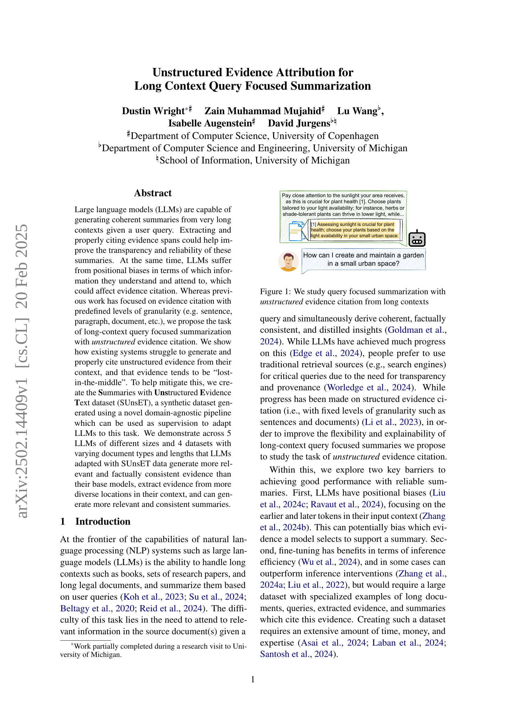
🔼 This figure illustrates the core task of the paper: query-focused summarization with unstructured evidence citation from lengthy source texts. It shows an example of a user query alongside a long excerpt from a document and highlights the challenge of generating a summary that accurately reflects the document’s information while also citing the specific parts of the document that support the summary’s claims. The unstructured nature emphasizes that the cited evidence doesn’t need to adhere to any pre-defined structure (like sentences or paragraphs), making the task more complex and flexible.
read the caption
Figure 1: We study query focused summarization with unstructured evidence citation from long contexts
| SUnsET | Base | Base w/ Titles | ||||||||||
|---|---|---|---|---|---|---|---|---|---|---|---|---|
| Method | Titles | Questions | Summaries | Documents | Titles | Questions | Summaries | Documents | Titles | Questions | Summaries | Documents |
| Moving Avg. TTR | 0.816 | 0.751 | 0.836 | 0.820 | 0.387 | 0.670 | 0.797 | 0.350 | 0.588 | 0.631 | 0.778 | 0.352 |
| Avg. Cosinse Dist. | 0.780 | 0.806 | 0.733 | 0.682 | 0.425 | 0.725 | 0.716 | 0.042 | 0.607 | 0.660 | 0.610 | 0.040 |
| Avg. Length (in words) | 5.44 | 13.45 | 226.5 | 3767.4 | 6.65 | 9.85 | 23.79 | 474.8 | 5.76 | 10.21 | 24.45 | 433.8 |
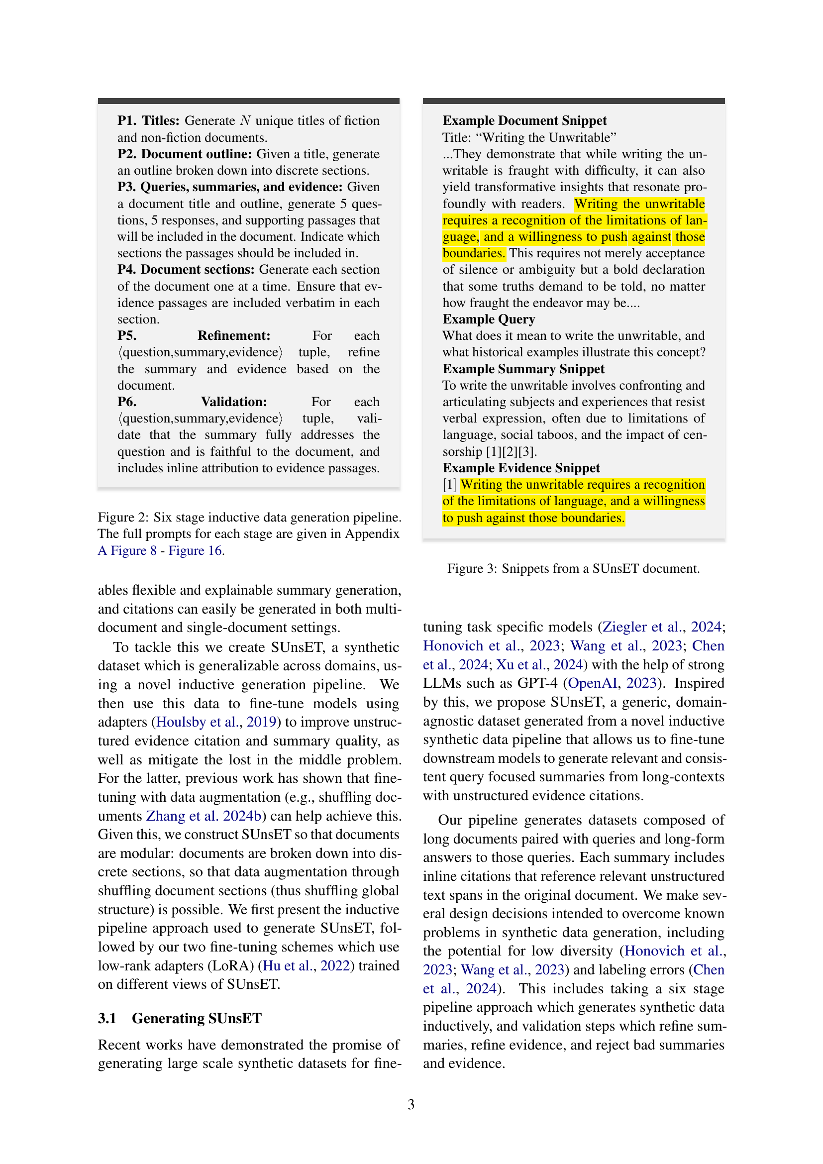
🔼 This table presents a statistical overview of the synthetic dataset generated for the study, focusing on the diversity and quality of the generated data. It includes metrics such as the average type-token ratio (TTR), average cosine distance between generated items, and the average lengths (in words) of titles, questions, summaries, and documents. The data are broken down by different generation methods to highlight the impact of the generation pipeline on data quality and diversity.
read the caption
Table 1: Statistics and diversity metrics of synthetically generated data.
In-depth insights#
Unstruct. Cite.#
I do not see a heading called ‘Unstruct. Cite.’ in this document. However, based on the context of the paper which is ‘Unstructured Evidence Attribution for Long Context Query Focused Summarization’, it appears the work would involve unstructured citation of data from within long documents. Models adapted to this task generate more relevant and factually consistent evidence. They extract evidence from diverse context locations and generate more relevant and consistent summaries. The results show improvements in transparency and reliability of summaries. Positional biases (lost in the middle) may be mitigated by using the new synthetic dataset generation SUnsET.
Lost in Middle#
Lost in the Middle refers to a common challenge in processing long sequences, where models struggle to effectively utilize information present in the middle segments. This often happens because attention mechanisms, which are crucial for capturing relationships between different parts of the input, may prioritize the beginning and end of the sequence, leading to a diminished focus on the intermediate content. The result is that relevant details or crucial context from the middle sections are overlooked, hindering the model’s ability to fully understand and generate coherent summaries or responses. Mitigating this requires techniques such as position-aware training, data shuffling, or architectural modifications to ensure more uniform attention distribution across the entire input sequence, thereby improving overall performance and reducing bias.
SUnsET Dataset#
The SUnsET dataset is a novel, synthetically generated resource designed to train language models for unstructured evidence citation in long-context summarization. It addresses the challenges of positional bias and the need for large, specialized datasets. The dataset’s construction employs a domain-agnostic, inductive pipeline, focusing on flexibility and explainability. Its modular design, with documents broken into discrete sections, enables data augmentation through shuffling, mitigating positional biases. The pipeline involves multiple stages including title generation, document outlining, query/summary creation, section generation, refinement, and validation. Fine-tuning models on SUnsET enhances their ability to extract relevant evidence, improve summary quality, and mitigate the “lost-in-the-middle” issue by providing better citations.
Adapter Tuning#
Adapter tuning, particularly using techniques like LoRA, emerges as a cost-effective strategy for adapting LLMs to specialized tasks, such as unstructured evidence attribution. This approach is more parameter-efficient than full fine-tuning. Adapters work by inserting new layers into the original model to extract better results, thus reducing computational resources. Additionally, adapters can mitigate the lost-in-the-middle problem, helping models use unstructured evidence. Different adapter training regimes, such as position-aware and position-agnostic training, can impact performance, with position-aware training potentially enhancing evidence quality and position-agnostic training mitigating positional biases. The success depends on data quality and domain relevance. It also allows for a dynamic trade-off between resource efficiency and high performance.
Reduce Bias#
While the paper doesn’t explicitly have a section titled “Reduce Bias,” the concept is woven throughout. The core contribution—unstructured evidence attribution—aims to increase transparency, which inherently combats bias by revealing the source of information. By citing specific text spans, the model’s reasoning becomes more auditable, reducing the risk of it presenting biased summaries based on selectively chosen or misinterpreted evidence. The paper acknowledges positional bias in LLMs, where they favor information at the beginning or end of the context. Their proposed SUnsET dataset and shuffling strategies are direct attempts to mitigate this bias. The paper also touches on ethical considerations related to plagiarism and copyright, underscoring the need for careful attention to potential biases introduced during synthetic data generation. The paper argues that careful tuning with data augmentation can further reduce evidence bias.
More visual insights#
More on figures

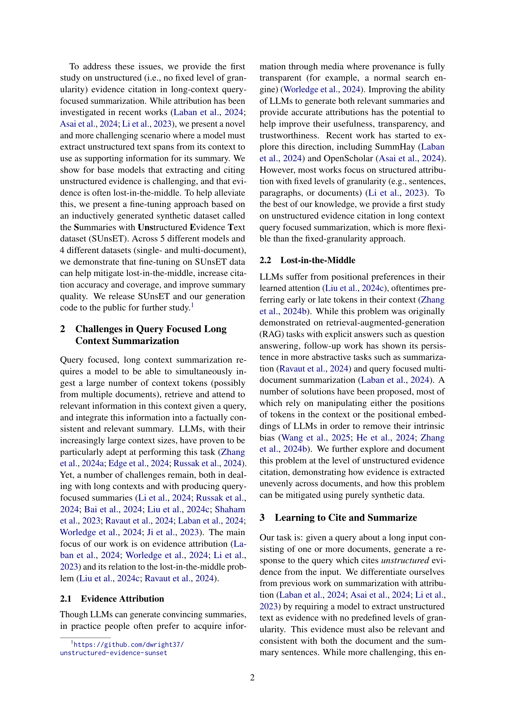
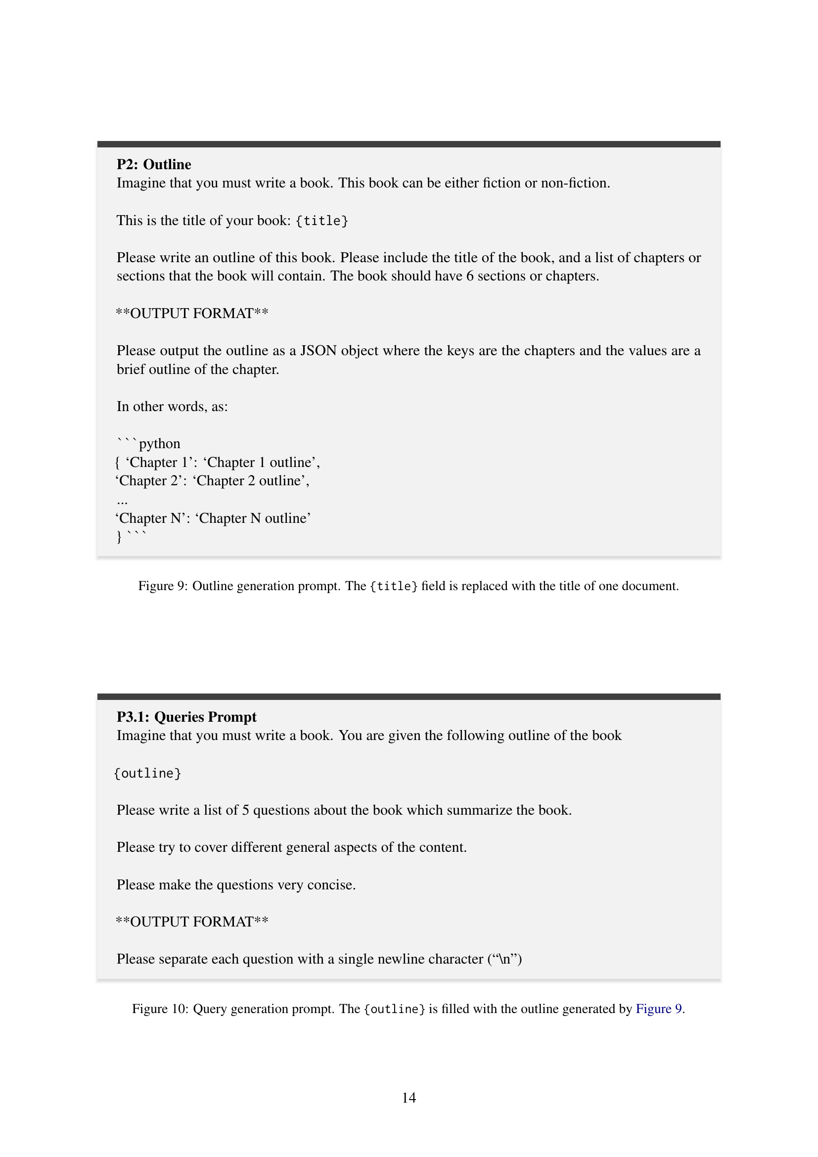
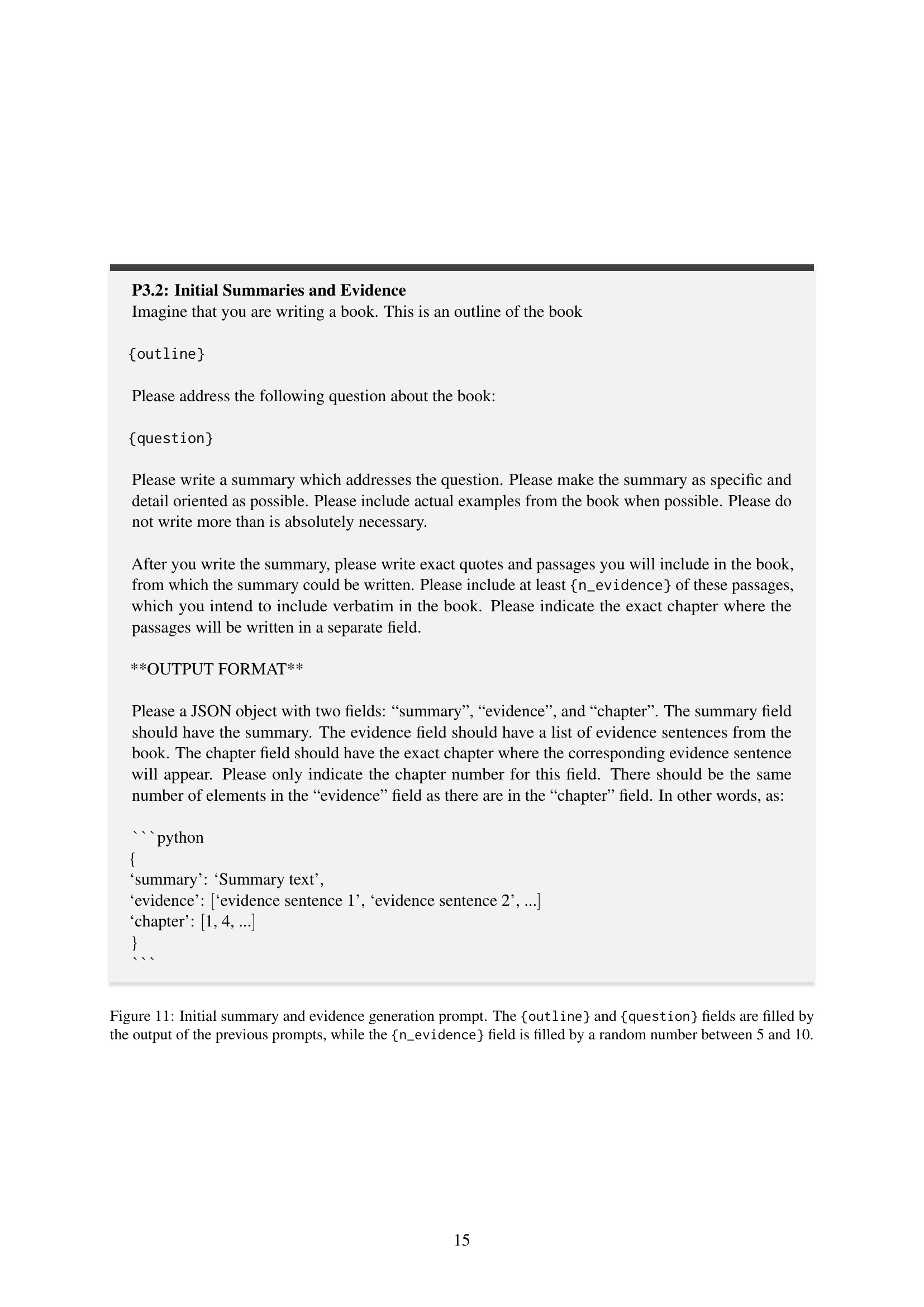
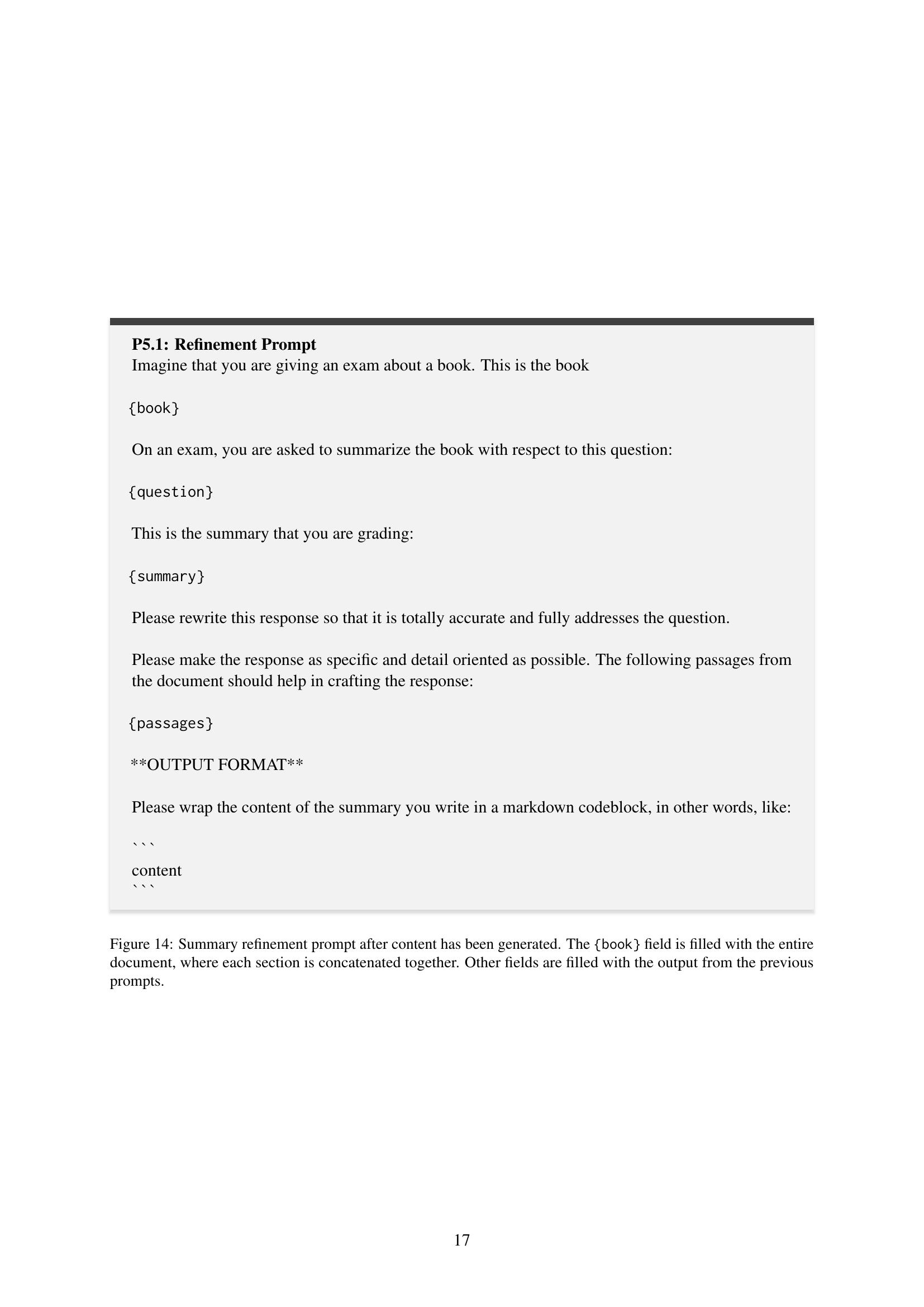
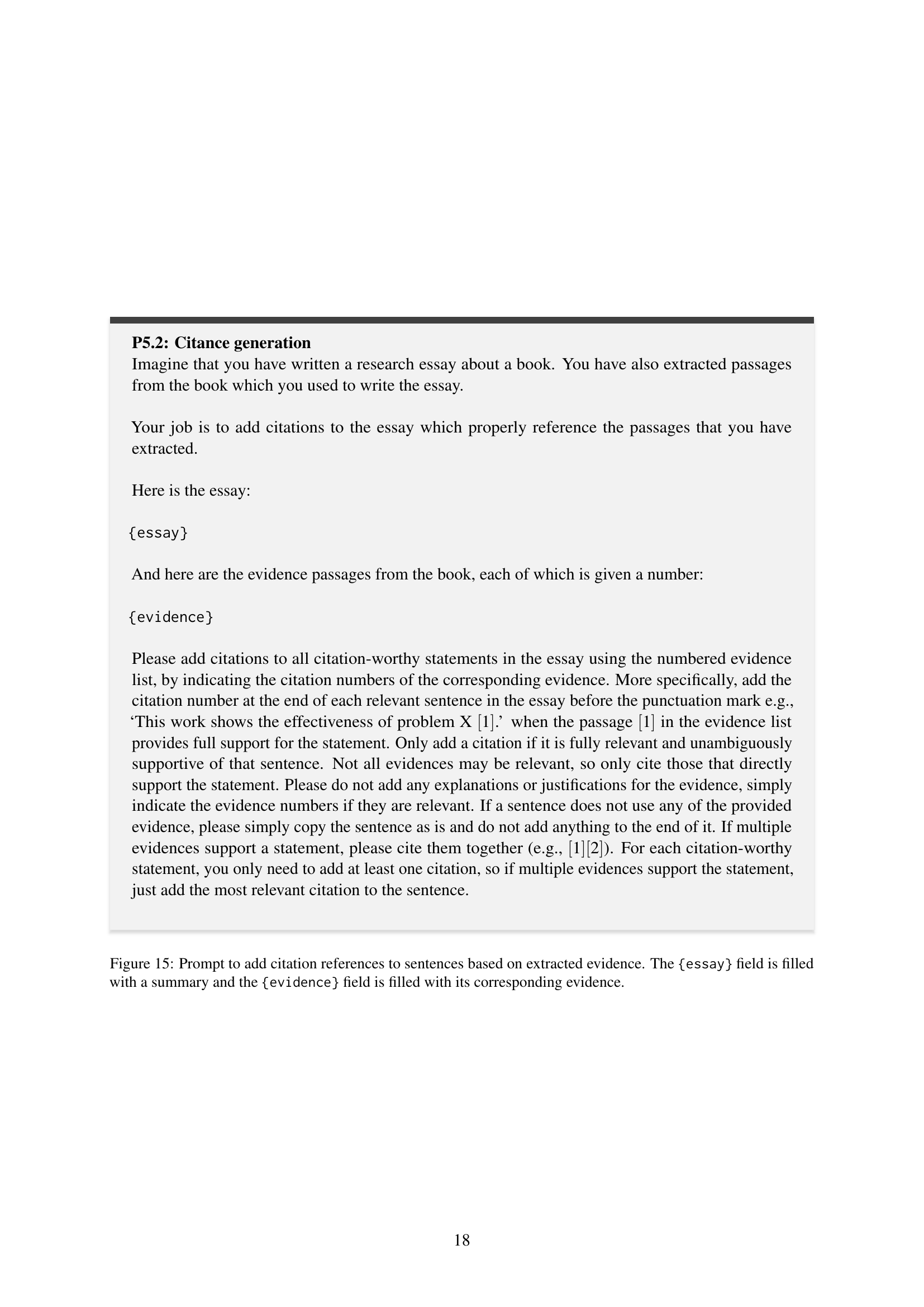
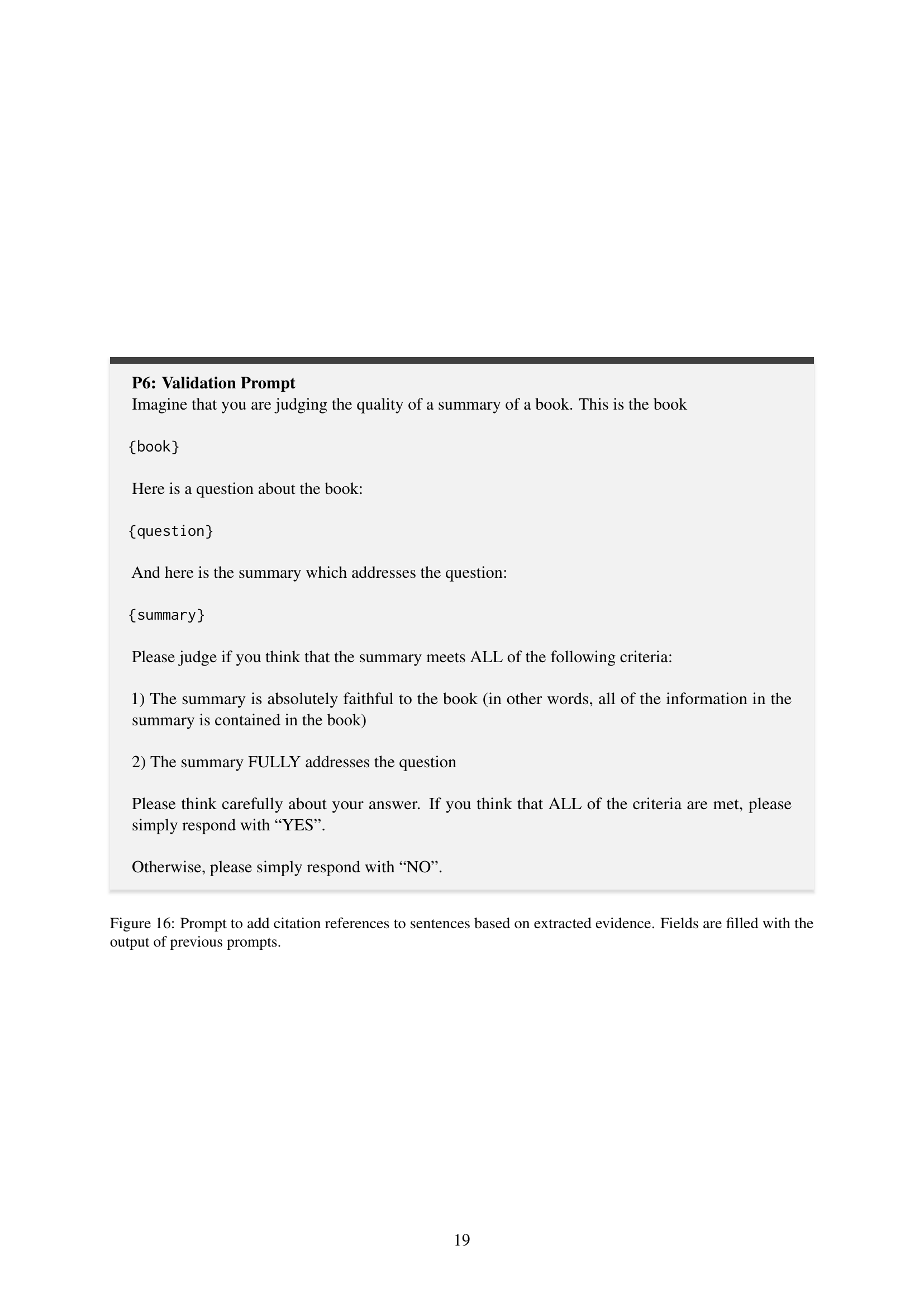
🔼 This figure illustrates the six-stage pipeline used to generate the Summaries with Unstructured Evidence Text (SUnsET) dataset. Each stage involves a different prompt to a large language model (LLM), generating various components of the dataset. The process begins with generating unique titles for fictional and non-fiction documents (P1). An outline of each document is then created (P2), followed by the generation of queries, summaries, and supporting evidence passages (P3). The evidence passages are then incorporated into the actual document sections (P4). Subsequently, the summaries and evidence are refined based on the completed document (P5). Finally, the generated data is validated to ensure that the summaries are accurate and the evidence is properly cited (P6). The prompts used in each of these six stages are detailed in Appendix A (Figures 8-16).
read the caption
Figure 2: Six stage inductive data generation pipeline. The full prompts for each stage are given in Appendix A Figure 8 - Figure 16.

🔼 This figure shows example snippets from a document in the SUnsET dataset. It illustrates the structure of a SUnsET document, including the title, a section of the document text, an example query related to the document’s content, a snippet of a generated summary that answers the query, and a snippet of the evidence used to support the summary. The snippets highlight the unstructured nature of the evidence citation within the SUnsET dataset.
read the caption
Figure 3: Snippets from a SUnsET document.

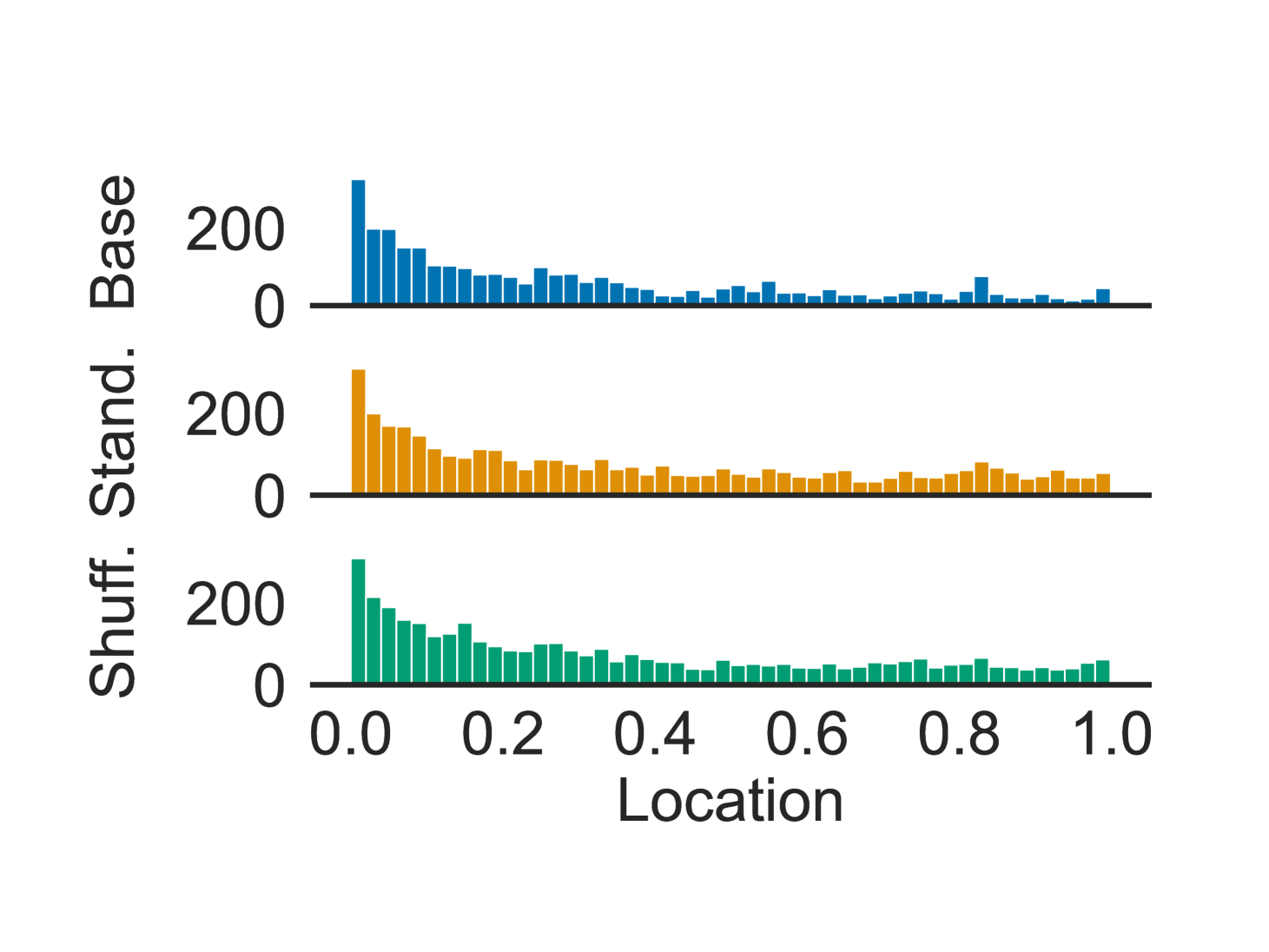
🔼 This figure shows the distribution of extracted evidence locations within the source document for the Llama 3.2 1B model using three different methods: standard training, shuffled training, and the base model without fine-tuning. The x-axis represents the relative location of the extracted evidence within the document (0.0 being the beginning and 1.0 being the end), and the y-axis represents the count of extracted evidence at each location. The figure helps visualize the impact of training methods on the positional bias of the model, showing whether the model tends to extract evidence from specific parts of the document (e.g., the beginning or end) or distributes evidence extraction more evenly across the document.
read the caption
(a) Llama 3.2 1B

🔼 This histogram displays the distribution of extracted evidence locations within the source document for the Llama 3.2 3B model. The x-axis represents the relative location of the evidence within the document (0.0 being the beginning and 1.0 being the end), and the y-axis shows the frequency or count of extracted evidence at each location. Three sets of results are shown: the base model (without fine-tuning on the SUnsET dataset), the model fine-tuned with standard context, and the model fine-tuned with shuffled context. The figure helps visualize the model’s tendency to focus on specific locations within the document when extracting evidence (positional bias), and the effect of different fine-tuning methods on this bias. Comparing this to the distribution of ground truth evidence in Figure 5 allows for a more direct assessment of the model’s performance.
read the caption
(b) Llama 3.2 3B
🔼 This figure is a histogram showing the distribution of extracted evidence locations within the provided source context for the Llama 3.1 8B model. The x-axis represents the relative location of the extracted evidence (0.0 being the beginning and 1.0 being the end of the document), and the y-axis represents the count of evidence instances found at each location. The histogram compares three different methods: the base model, a model fine-tuned with standard context, and a model fine-tuned with shuffled context. This visualization helps to understand the model’s positional bias and the effectiveness of different fine-tuning methods in mitigating this bias.
read the caption
(c) Llama 3.1 8B

🔼 This figure is a histogram showing the distribution of extracted evidence locations within the provided source context for the Mistral Nemo 2407 model. The x-axis represents the location of the extracted evidence (normalized to the range [0, 1]), with 0 representing the beginning of the document and 1 representing the end. The y-axis shows the count of evidence instances at each location. The histogram allows for a visual comparison of the distribution of evidence across different extraction methods (standard, shuffled, and baseline). This aids in assessing the impact of the training method on the positioning of extracted evidence within the document, particularly relating to the ’lost-in-the-middle’ phenomenon discussed in the paper.
read the caption
(d) Mistral Nemo 2407

🔼 This histogram displays the distribution of extracted evidence locations within the source document for the Mixtral 8x7B model. The x-axis represents the relative location of the evidence within the document (0.0 being the beginning and 1.0 being the end), and the y-axis represents the count of evidence snippets found at each location. The bars are grouped into three categories: ‘Base’, representing the baseline model without fine-tuning; ‘Standard’, representing the model fine-tuned with the standard SUnsET dataset; and ‘Shuffled’, representing the model fine-tuned with the shuffled SUnsET dataset. This visualization helps to understand whether the model’s evidence selection exhibits positional bias (favoring evidence from the beginning or end of the document) and how fine-tuning with SUnsET data, with and without shuffling, affects this bias.
read the caption
(e) Mixtral 8x7B

🔼 This figure shows the distribution of extracted evidence locations within the source document for the GPT-40 mini model. The x-axis represents the location of evidence within the document, ranging from 0.0 (beginning) to 1.0 (end). The y-axis represents the count of extracted evidence spans found at each location. The bars show the distribution for three different methods: Base (the original, unadapted model), Standard (fine-tuned with SUnsET data), and Shuffled (fine-tuned with SUnsET data with shuffled document sections). This visualization helps illustrate the presence of positional bias (lost-in-the-middle) in language models and the effect of the proposed fine-tuning method on mitigating this bias.
read the caption
(f) GPT 4o Mini

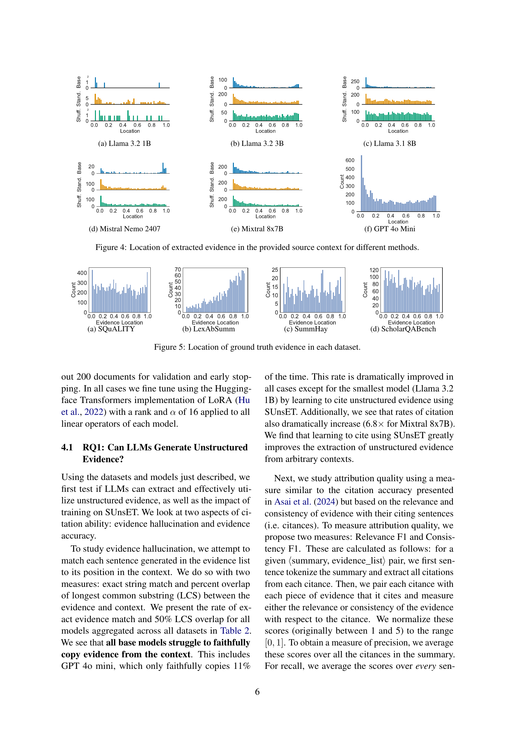
🔼 This figure displays histograms showing the distribution of extracted evidence locations within source documents for various methods. Each histogram represents a different large language model (LLM) and shows the relative frequency of evidence extracted from different positions (beginning, middle, or end) within the document. The comparison allows for analysis of how different LLMs and processing techniques (such as standard vs. shuffled fine-tuning) affect where evidence is selected from within a given document context.
read the caption
Figure 4: Location of extracted evidence in the provided source context for different methods.
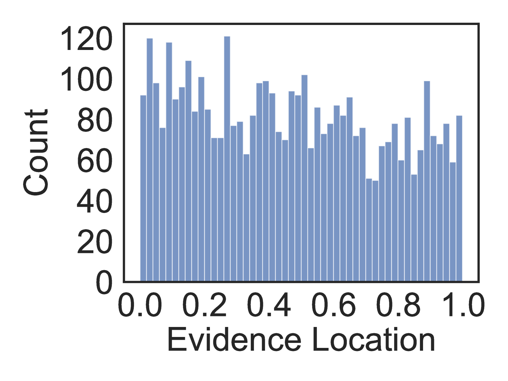
🔼 This figure shows the distribution of ground truth evidence locations within the SQuALITY dataset. The x-axis represents the relative location of the evidence within the document, ranging from 0.0 (beginning) to 1.0 (end). The y-axis shows the count of evidence instances at each location. The figure helps visualize the distribution of evidence across different sections of the documents in this dataset, indicating whether there’s a bias toward the beginning, middle, or end of the documents.
read the caption
(a) SQuALITY

🔼 Figure 5(b) shows the distribution of ground truth evidence locations in the LexAbSumm dataset. LexAbSumm consists of long legal documents, focusing on the location of evidence within those documents. The x-axis represents the relative location of evidence within the document (from 0.0 to 1.0), and the y-axis represents the count of evidence at each location. This visualization helps illustrate the distribution of evidence throughout the documents and can be used to understand any positional biases present in the data or in models trained on this data. The graph shows a relatively uniform distribution of evidence across the documents, suggesting there is no strong positional bias towards either the beginning or end of the documents within this dataset.
read the caption
(b) LexAbSumm

🔼 The figure shows the distribution of ground truth evidence locations in the SummHay dataset. The x-axis represents the relative location of evidence within the document (0.0 being the beginning and 1.0 being the end). The y-axis represents the count of evidence instances at each location. The distribution illustrates where the actual evidence is present in the documents, helping to understand any inherent biases in evidence placement within the dataset.
read the caption
(c) SummHay

🔼 Figure 5(d) presents the distribution of ground truth evidence locations within the ScholarQABench dataset. ScholarQABench is a multi-document dataset consisting of computer science research papers. The x-axis represents the relative location of evidence within a document (0.0 being the beginning, 1.0 being the end), and the y-axis represents the count of evidence instances at each location. This visualization helps to understand the distribution of evidence within the documents of this specific dataset, allowing for a comparison with the distribution of evidence extracted by different LLMs (as shown in other subfigures of Figure 5 and Figure 4).
read the caption
(d) ScholarQABench
🔼 This figure presents four histograms, one for each of the datasets used in the study (SQUALITY, LexAbSumm, SummHay, and ScholarQABench). Each histogram visualizes the distribution of ground truth evidence locations within the documents of the corresponding dataset. The x-axis represents the relative location of the evidence within the document (0.0 being the beginning and 1.0 being the end), and the y-axis represents the count of evidence instances at each location. This figure helps illustrate whether there’s a bias in the location of evidence within documents, which is related to the ’lost-in-the-middle’ phenomenon discussed in the paper.
read the caption
Figure 5: Location of ground truth evidence in each dataset.

🔼 This figure shows the location of extracted evidence within the source document for the Llama 3.2 1B model. The x-axis represents the relative location of the evidence in the document (0.0 being the beginning and 1.0 being the end). The y-axis shows the count of evidence extracted at each location. Three bars are shown for each model: ‘Base’ (the unembellished model), ‘Standard’ (fine-tuned with SUnsET data in its original order), and ‘Shuffled’ (fine-tuned with SUnsET data with sections randomly shuffled). This visualization helps illustrate the effect of fine-tuning and shuffled training on the tendency of the model to extract evidence primarily from the beginning or end of the document (’lost-in-the-middle’ effect).
read the caption
(a) Llama 3.2 1B

🔼 This figure is a histogram showing the location of extracted evidence within the source document for the Llama 3.1 8B language model. The x-axis represents the relative location of evidence in the document (0.0 being the beginning, 1.0 being the end), and the y-axis represents the count of evidence instances found at each location. The histogram compares the distribution of evidence extracted by three different methods: the base model, the model fine-tuned with standard context, and the model fine-tuned with shuffled context. The purpose is to visualize the impact of different fine-tuning methods on the positional bias of the model in evidence extraction.
read the caption
(b) Llama 3.1 8B
More on tables
| Method | Exact Match | 50% Match | # Evidence |
| Llama 3.2 1B | 0.0 | 35.71 | 14 |
| + Standard | 7.69 | 43.26 | 208 |
| + Shuffled | 5.15 | 22.68 | 97 |
| Llama 3.2 3B | 25.57 | 90.11 | 1345 |
| + Standard | 52.77 | 85.62 | 3720 |
| + Shuffled | 32.99 | 74.07 | 2337 |
| Llama 3.1 8B | 43.93 | 83.12 | 3412 |
| + Standard | 78.36 | 97.21 | 4690 |
| + Shuffled | 54.53 | 88.51 | 4684 |
| Mistral Nemo 2407 | 5.48 | 66.13 | 310 |
| + Standard | 82.20 | 97.29 | 2107 |
| + Shuffled | 72.38 | 95.76 | 1959 |
| Mixtral 8x7B | 5.79 | 91.25 | 3452 |
| + Standard | 33.82 | 90.47 | 4208 |
| + Shuffled | 29.29 | 90.74 | 4288 |
| GPT-4o-mini | 11.06 | 96.32 | 8159 |
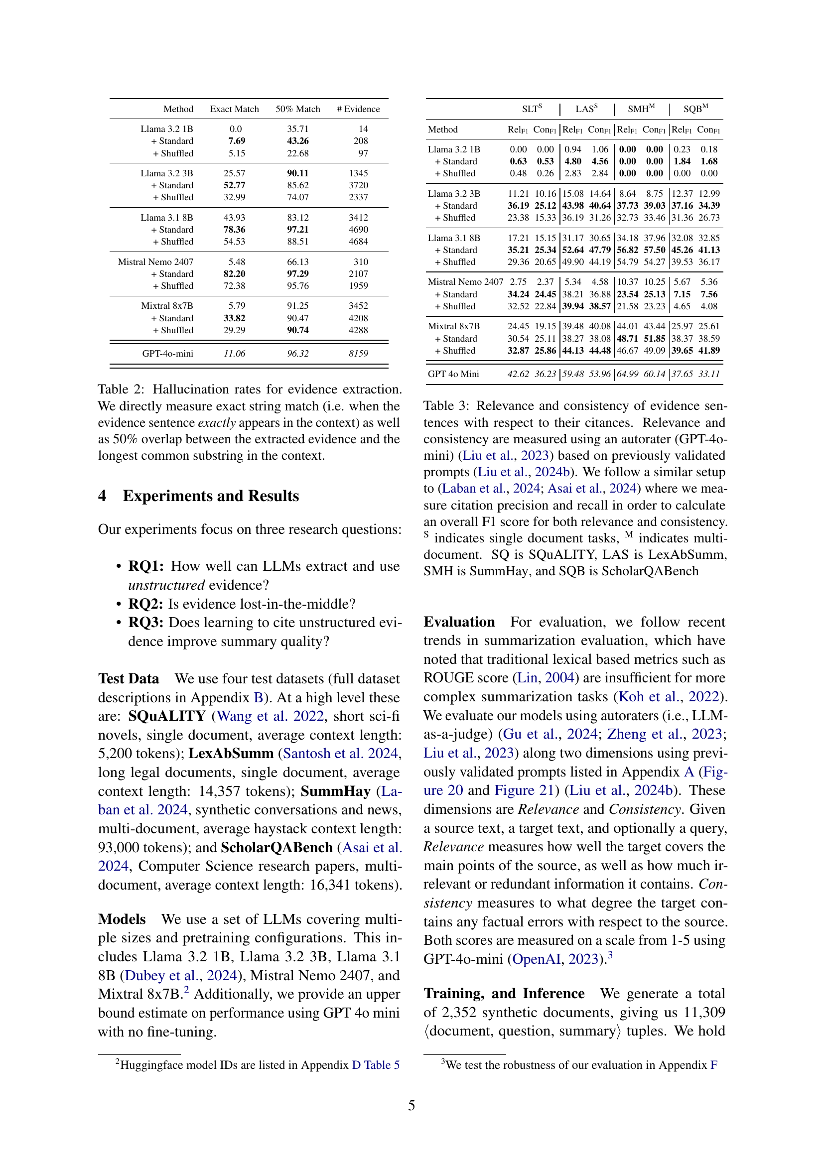
🔼 Table 2 presents the hallucination rates of evidence extraction performed by different LLMs. It measures the accuracy of evidence extraction in two ways: exact string match (where the extracted evidence is identical to a sentence in the source text) and 50% overlap (where the extracted evidence has at least a 50% overlap with the longest common substring in the source text). This provides a comprehensive evaluation of how well the models accurately extract evidence from the source documents, helping to identify cases of hallucination (where the model generates evidence not present in the source).
read the caption
Table 2: Hallucination rates for evidence extraction. We directly measure exact string match (i.e. when the evidence sentence exactly appears in the context) as well as 50% overlap between the extracted evidence and the longest common substring in the context.
| SLTS | LASS | SMHM | SQBM | |||||
| Method | RelF1 | ConF1 | RelF1 | ConF1 | RelF1 | ConF1 | RelF1 | ConF1 |
| Llama 3.2 1B | 0.00 | 0.00 | 0.94 | 1.06 | 0.00 | 0.00 | 0.23 | 0.18 |
| + Standard | 0.63 | 0.53 | 4.80 | 4.56 | 0.00 | 0.00 | 1.84 | 1.68 |
| + Shuffled | 0.48 | 0.26 | 2.83 | 2.84 | 0.00 | 0.00 | 0.00 | 0.00 |
| Llama 3.2 3B | 11.21 | 10.16 | 15.08 | 14.64 | 8.64 | 8.75 | 12.37 | 12.99 |
| + Standard | 36.19 | 25.12 | 43.98 | 40.64 | 37.73 | 39.03 | 37.16 | 34.39 |
| + Shuffled | 23.38 | 15.33 | 36.19 | 31.26 | 32.73 | 33.46 | 31.36 | 26.73 |
| Llama 3.1 8B | 17.21 | 15.15 | 31.17 | 30.65 | 34.18 | 37.96 | 32.08 | 32.85 |
| + Standard | 35.21 | 25.34 | 52.64 | 47.79 | 56.82 | 57.50 | 45.26 | 41.13 |
| + Shuffled | 29.36 | 20.65 | 49.90 | 44.19 | 54.79 | 54.27 | 39.53 | 36.17 |
| Mistral Nemo 2407 | 2.75 | 2.37 | 5.34 | 4.58 | 10.37 | 10.25 | 5.67 | 5.36 |
| + Standard | 34.24 | 24.45 | 38.21 | 36.88 | 23.54 | 25.13 | 7.15 | 7.56 |
| + Shuffled | 32.52 | 22.84 | 39.94 | 38.57 | 21.58 | 23.23 | 4.65 | 4.08 |
| Mixtral 8x7B | 24.45 | 19.15 | 39.48 | 40.08 | 44.01 | 43.44 | 25.97 | 25.61 |
| + Standard | 30.54 | 25.11 | 38.27 | 38.08 | 48.71 | 51.85 | 38.37 | 38.59 |
| + Shuffled | 32.87 | 25.86 | 44.13 | 44.48 | 46.67 | 49.09 | 39.65 | 41.89 |
| GPT 4o Mini | 42.62 | 36.23 | 59.48 | 53.96 | 64.99 | 60.14 | 37.65 | 33.11 |
🔼 This table presents the results of evaluating the relevance and consistency of evidence sentences generated by different models in relation to their corresponding citations. The evaluation uses an automated system (GPT-40-mini) and employs previously validated prompts. The methodology aligns with similar studies by Laban et al. (2024) and Asai et al. (2024), calculating F1 scores (combining precision and recall) for both relevance and consistency of the citations. The table also specifies whether the task involved single or multiple documents and uses abbreviations to identify the datasets used (SQuALITY, LexAbSumm, SummHay, and ScholarQABench).
read the caption
Table 3: Relevance and consistency of evidence sentences with respect to their citances. Relevance and consistency are measured using an autorater (GPT-4o-mini) Liu et al. (2023) based on previously validated prompts Liu et al. (2024b). We follow a similar setup to Laban et al. (2024); Asai et al. (2024) where we measure citation precision and recall in order to calculate an overall F1 score for both relevance and consistency. S indicates single document tasks, M indicates multi-document. SQ is SQuALITY, LAS is LexAbSumm, SMH is SummHay, and SQB is ScholarQABench
| SLTS | LASS | SMHM | SQBM | |||||
| Method | Rel | Con | Rel | Con | Rel | Con | Rel | Con |
| Llama 3.2 1B | 2.68 | 2.15 | 3.68 | 3.38 | 4.53 | 4.40 | 3.80 | 3.61 |
| + Standard | 2.73= | 2.17= | 3.25 | 2.93 | 4.53= | 4.44= | 3.81= | 3.59= |
| + Shuffled | 2.79* | 2.15= | 3.41 | 3.03 | 4.66* | 4.55* | 3.97* | 3.69* |
| Llama 3.2 3B | 4.39 | 4.05 | 4.40 | 4.19 | 4.82 | 4.74 | 4.28 | 4.11 |
| + Standard | 4.22 | 3.80 | 4.19 | 4.02 | 4.90* | 4.85* | 4.41* | 4.21* |
| + Shuffled | 3.84 | 3.38 | 4.25 | 4.02 | 4.89* | 4.84* | 4.49* | 4.23* |
| Llama 3.1 8B | 4.55 | 4.34 | 4.64 | 4.52 | 4.88 | 4.78 | 4.18 | 4.06 |
| + Standard | 4.63* | 4.41* | 4.53 | 4.44 | 4.94* | 4.93* | 4.64* | 4.42* |
| + Shuffled | 4.59* | 4.34= | 4.55 | 4.44 | 4.97* | 4.92* | 4.68* | 4.41* |
| Mistral Nemo 2407 | 4.27 | 4.09 | 3.83 | 3.85 | 4.27 | 4.15 | 3.15 | 3.23 |
| + Standard | 4.43* | 4.24* | 4.03* | 4.04* | 4.54* | 4.47* | 3.79* | 3.75* |
| + Shuffled | 4.53* | 4.35* | 4.18* | 4.12* | 4.65* | 4.49* | 3.49* | 3.41* |
| Mixtral 8x7B | 4.02 | 3.99 | 4.28 | 4.22 | 4.78 | 4.68 | 3.95 | 3.89 |
| + Standard | 4.52* | 4.35* | 4.45* | 4.40* | 4.84* | 4.72* | 4.26* | 4.13* |
| + Shuffled | 4.51* | 4.40* | 4.44* | 4.38* | 4.79= | 4.68= | 4.33* | 4.18* |
| GPT 4o Mini | 4.98 | 4.92 | 4.93 | 4.77 | 4.99 | 4.98 | 4.94 | 4.76 |
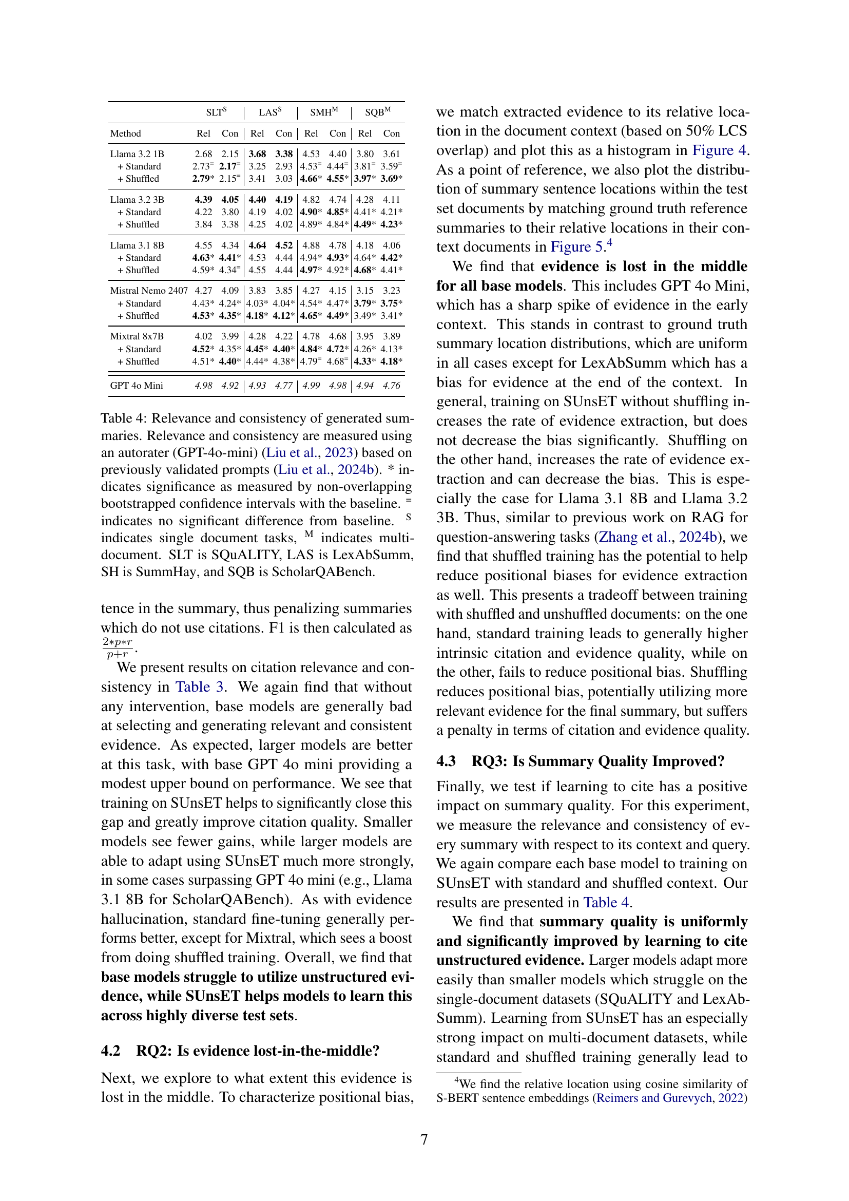
🔼 Table 4 presents the results of evaluating the relevance and consistency of summaries generated by different LLMs. Relevance and consistency were assessed using an automatic evaluator (GPT-4o-mini) and previously validated prompts. Statistical significance was determined using non-overlapping bootstrapped confidence intervals. The table includes results for four datasets, categorized as single-document or multi-document tasks. Abbreviations for the datasets are provided.
read the caption
Table 4: Relevance and consistency of generated summaries. Relevance and consistency are measured using an autorater (GPT-4o-mini) Liu et al. (2023) based on previously validated prompts Liu et al. (2024b). * indicates significance as measured by non-overlapping bootstrapped confidence intervals with the baseline. = indicates no significant difference from baseline. S indicates single document tasks, M indicates multi-document. SLT is SQuALITY, LAS is LexAbSumm, SH is SummHay, and SQB is ScholarQABench.
| Model | Huggingface Identifier |
|---|---|
| Llama 3.2 1B | meta-llama/Llama-3.2-1B-Instruct |
| Llama 3.2 3B | meta-llama/Llama-3.2-3B-Instruct |
| Llama 3.1 8B | meta-llama/Meta-Llama-3.1-8B-Instruct |
| Mistral Nemo 2407 | mistralai/Mistral-Nemo-Instruct-2407 |
| Mixtral 8x7B | mistralai/Mixtral-8x7B-Instruct-v0.1 |
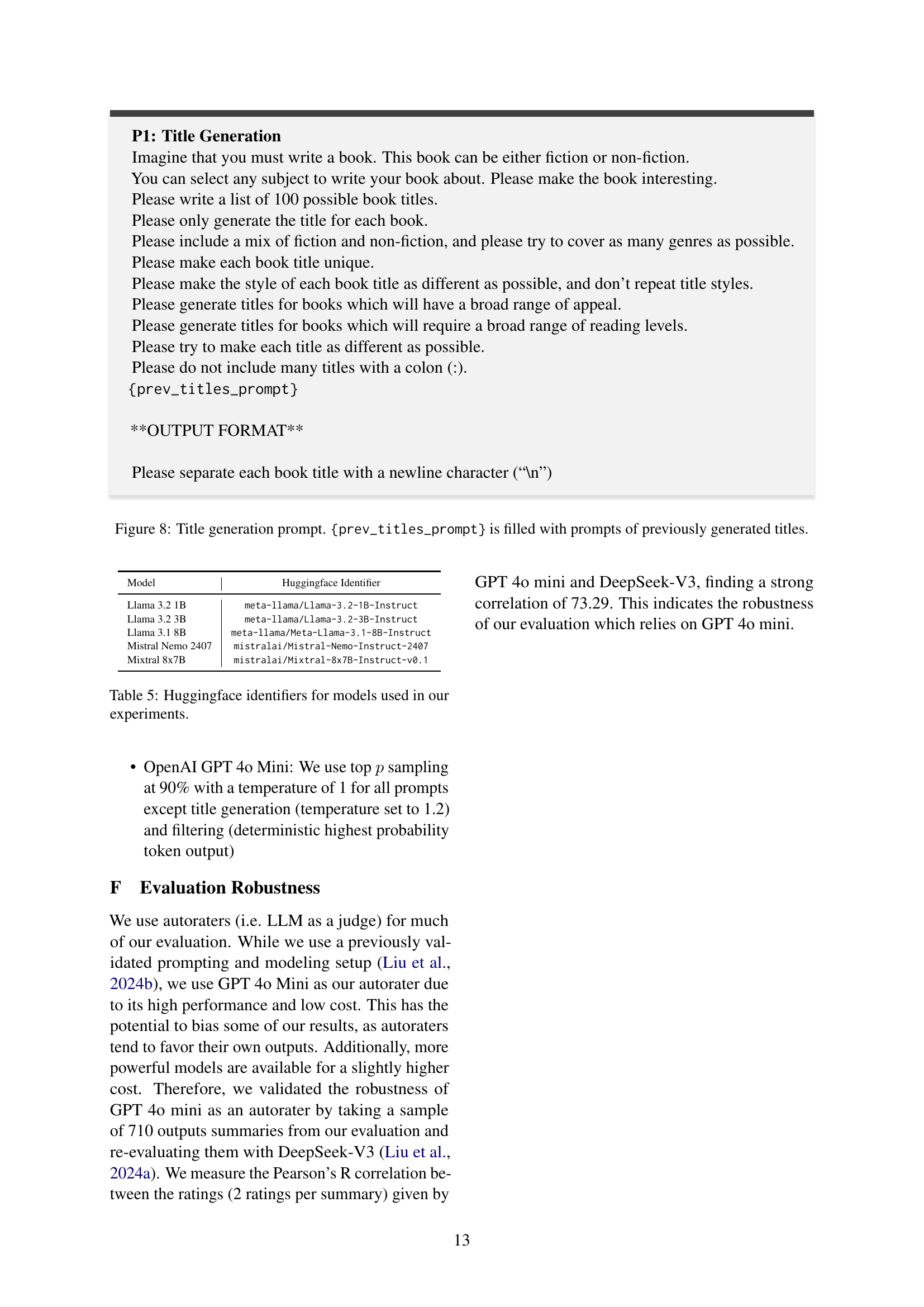
🔼 This table lists the Hugging Face model identifiers used in the paper’s experiments. For each model, the identifier is provided, allowing researchers to easily locate and access the specific model version used for reproducibility. The models represent a range of sizes and architectures, offering a comprehensive comparison across different LLMs.
read the caption
Table 5: Huggingface identifiers for models used in our experiments.
Full paper#