RectifiedHR: Enable Efficient High-Resolution Image Generation via Energy Rectification

2503.02537

Zhen Yang et el.

🤗 2025-03-05

TL;DR
#

Diffusion models excel in image generation, but struggle at higher resolutions than their training data. Existing solutions are inefficient or complex. This paper introduces RectifiedHR to address this issue. RectifiedHR is a training-free method for high-resolution image generation. It introduces a Noise Refresh strategy, requiring minimal code to improve resolution and efficiency.

RectifiedHR addresses the energy decay phenomenon that causes blurriness. It employs an Energy Rectification strategy, adjusting classifier-free guidance to enhance performance. The method is training-free, boasts simple logic, and demonstrates effectiveness and efficiency compared to baselines. It achieves superior results through a simple and efficient framework.

Key Takeaways
#

Why does it matter?
#

This paper introduces RectifiedHR, a practical approach to high-resolution image generation. By offering a training-free and efficient solution, it enables exploration of model capabilities without extensive retraining or complex setups, fostering advancements in generative AI.

Visual Insights
#

🔼 This figure showcases example images generated using the RectifiedHR method. The images demonstrate the method’s capability to produce high-resolution outputs (significantly larger than the training resolution of the underlying diffusion model, SDXL) without requiring any additional training. The diverse range of subjects and visual styles highlight the method’s versatility. The caption encourages viewers to zoom in for a closer inspection of the image details.
read the caption
Figure 1: Generated images of our method. Our training-free method can enable diffusion models (SDXL in the figure) to generate images at resolutions higher than their original training resolution. ZOOM IN for a closer look.

	Methods	$\mathrm{FID}_{r}\downarrow$	$\mathrm{KID}_{r}\downarrow$	$\mathrm{IS}_{r}\uparrow$	$\mathrm{FID}_{c}\downarrow$	$\mathrm{KID}_{c}\downarrow$	$\mathrm{IS}_{c}\uparrow$	CLIP $\uparrow$	Time $\downarrow$
2048x2048	FouriScale	71.344	0.010	15.957	53.990	0.014	20.625	31.157	59s
	ScaleCrafter	64.236	0.007	15.952	45.861	0.010	22.252	31.803	35s
	HiDiffusion	63.674	0.007	16.876	41.930	0.008	23.165	31.711	18s
	CutDiffusion	59.152	0.007	17.109	38.004	0.008	23.444	32.573	53s
	ElasticDiffusion	56.639	0.010	15.326	37.649	0.014	19.867	32.301	150s
	AP-LDM	51.083	0.004	18.867	29.193	0.006	25.331	33.601	25s
	AccDiffusion	48.143	0.002	18.466	32.747	0.008	24.778	33.153	111s
	DiffuseHigh	49.748	\ul0.003	19.537	27.667	\ul0.004	27.876	33.436	37s
	FreCas	49.129	\ul0.003	20.274	27.002	\ul0.004	29.843	33.700	14s
	DemoFusion	47.079	0.002	19.533	26.441	\ul0.004	27.843	33.748	79s
	SDXL+BSRGAN	\ul47.452	0.002	\ul20.260	\ul25.827	\ul0.004	27.155	33.867	6s
	Ours	48.361	0.002	20.616	25.347	0.003	\ul28.126	\ul33.756	\ul13s
4096x4096	FouriScale	135.111	0.046	9.481	129.895	0.057	9.792	26.891	489s
	ScaleCrafter	110.094	0.028	10.098	112.105	0.043	11.421	27.809	528s
	HiDiffusion	93.515	0.024	11.878	120.170	0.058	11.272	27.853	71s
	CutDiffusion	130.207	0.055	9.334	113.033	0.055	10.961	26.734	193s
	ElasticDiffusion	101.313	0.056	9.406	111.102	0.089	7.627	27.725	400s
	AP-LDM	51.274	0.005	18.676	41.615	0.012	20.126	\ul33.632	153s
	AccDiffusion	54.918	0.005	17.444	60.362	0.023	16.370	32.438	826s
	DiffuseHigh	48.861	\ul0.003	19.716	40.267	\ul0.010	\ul21.550	33.390	190s
	FreCas	49.764	\ul0.003	18.656	39.047	\ul0.010	21.700	33.237	74s
	DemoFusion	48.983	\ul0.003	18.225	\ul38.136	\ul0.010	20.786	33.311	605s
	SDXL+BSRGAN	47.923	0.002	\ul19.815	41.126	0.014	19.231	33.874	6s
	Ours	\ul48.684	\ul0.003	20.352	35.718	0.009	20.819	33.415	\ul37s

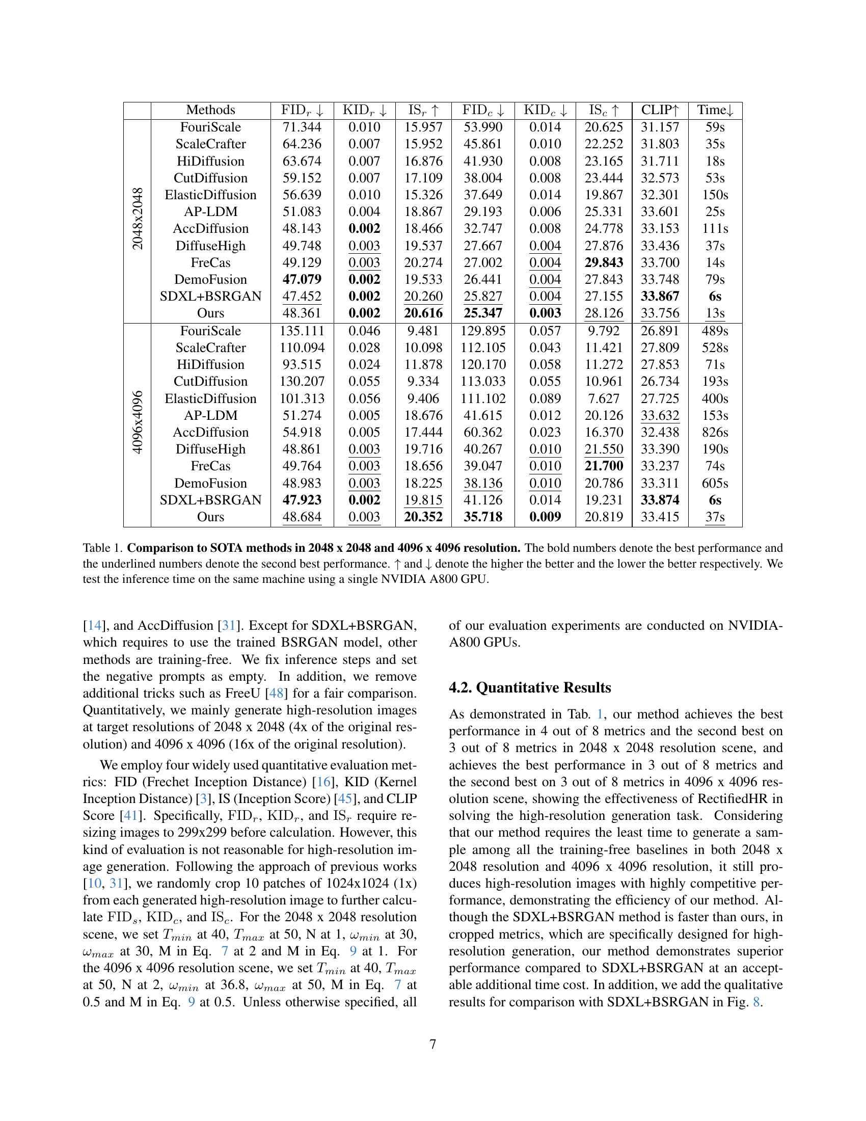
🔼 This table presents a quantitative comparison of the proposed RectifiedHR method against several state-of-the-art (SOTA) training-free high-resolution image generation methods. The comparison is performed at two resolutions: 2048x2048 and 4096x4096. The metrics used for evaluation include FID (Frechet Inception Distance), KID (Kernel Inception Distance), IS (Inception Score), and CLIP score. Lower FID and KID scores, and higher IS and CLIP scores indicate better performance. Inference time, measured on a single NVIDIA A800 GPU, is also included. The best and second-best results for each metric are highlighted in bold and underlined, respectively.
read the caption
Table 1: Comparison to SOTA methods in 2048 x 2048 and 4096 x 4096 resolution. The bold numbers denote the best performance and the underlined numbers denote the second best performance. ↑↑\uparrow↑ and ↓↓\downarrow↓ denote the higher the better and the lower the better respectively. We test the inference time on the same machine using a single NVIDIA A800 GPU.

In-depth insights
#

Energy Decay Info
#

The energy decay analysis is pivotal for understanding why naive implementations of high-resolution image generation, especially those involving techniques like noise refresh, can lead to blurring. The core idea is that as resolution increases, the latent space representation of the image loses energy, causing details to become indistinct. This contrasts with original sampling, where energy is maintained. Identifying this decay allows for targeted interventions, such as adjusting the classifier-free guidance (CFG) parameter. Increasing CFG strengthens the energy, thereby sharpening image details. This connection between energy levels, resolution, and CFG is crucial for developing effective high-resolution generation strategies.

Noise Refresh
#

The paper introduces a novel “Noise Refresh” technique, seemingly addressing limitations in high-resolution image generation using diffusion models. The approach likely involves re-introducing noise at specific points during the sampling process. This noise injection could help to refine details or correct structural inconsistencies that arise when extrapolating beyond the training resolution. The decision to apply noise refresh in the latter half of denoising suggests a focus on local detail enhancement, acknowledging that the global structure is largely formed in earlier stages. By converting the predicted ‘xo’ into RGB space for resizing, the method appears to be working directly with the image rather than in the latent space. The updated sampling formula indicates a way to inject noise that shares the same shape as the resized ‘xo’, preventing SNR mismatch issues. Overall, ‘Noise Refresh’ aims to enhance image clarity.

RectifiedHR
#

The name RectifiedHR suggests a method aimed at improving or ‘rectifying’ some aspect of High-Resolution image generation. The ‘HR’ clearly signals a focus on high-resolution imagery, implying the method addresses challenges specific to this domain. ‘Rectified’ hints at correcting distortions, artifacts, or inefficiencies. Perhaps the method aims to enhance image clarity, fidelity, or visual appeal. Alternatively, it might rectify issues related to computational cost, memory usage, or training instability. The choice of ‘Rectified’ also suggests a diagnostic approach; the method likely identifies and targets specific problems inherent in current HR image generation techniques, offering a solution to amend those limitations. It might deal with energy decay phenomenon and introduce noise refresh strategies to produce better high-resolution images.

No Training HR
#

The paper explores the exciting domain of training-free high-resolution image generation with their method RectifiedHR. This area is crucial because training models on high-resolution data is expensive. The method introduces a novel approach to unlock existing diffusion model’s ability to create HR images. It addresses a performance drop observed at higher resolutions and proposes a more efficient and straightforward solution compared to complex methods. By circumventing the need for extensive retraining, the approach promises reduced computational costs and broader accessibility. This highlights the potential for wider applications of HR image generation without huge investment, democratizing access to advanced generative capabilities.

Efficiency Boost
#

From the context of the paper focusing on high-resolution image generation using diffusion models, efficiency boosts likely refer to strategies that accelerate the image generation process without sacrificing quality. A key aspect could be reducing the number of diffusion steps required, possibly through techniques like noise refresh and energy rectification. Efficiency may also stem from a novel architecture or optimization that allows for faster processing of diffusion iterations, potentially by streamlining the computational demands of the U-Net. Furthermore, a key contribution of the work might be related to enhancing efficiency is the ability to generate high-resolution images without extensive retraining, leveraging knowledge learned from lower-resolution datasets. The integration of classifier-free guidance might also be optimized, allowing for high-quality generation without a significant increase in computational burden. This is supported by the novel training-free approach for efficient high-resolution image generation, which primarily includes noise refresh and energy rectification operations, requiring fewer lines of theoretical code to implement and is highly efficient.

More visual insights
#

More on figures

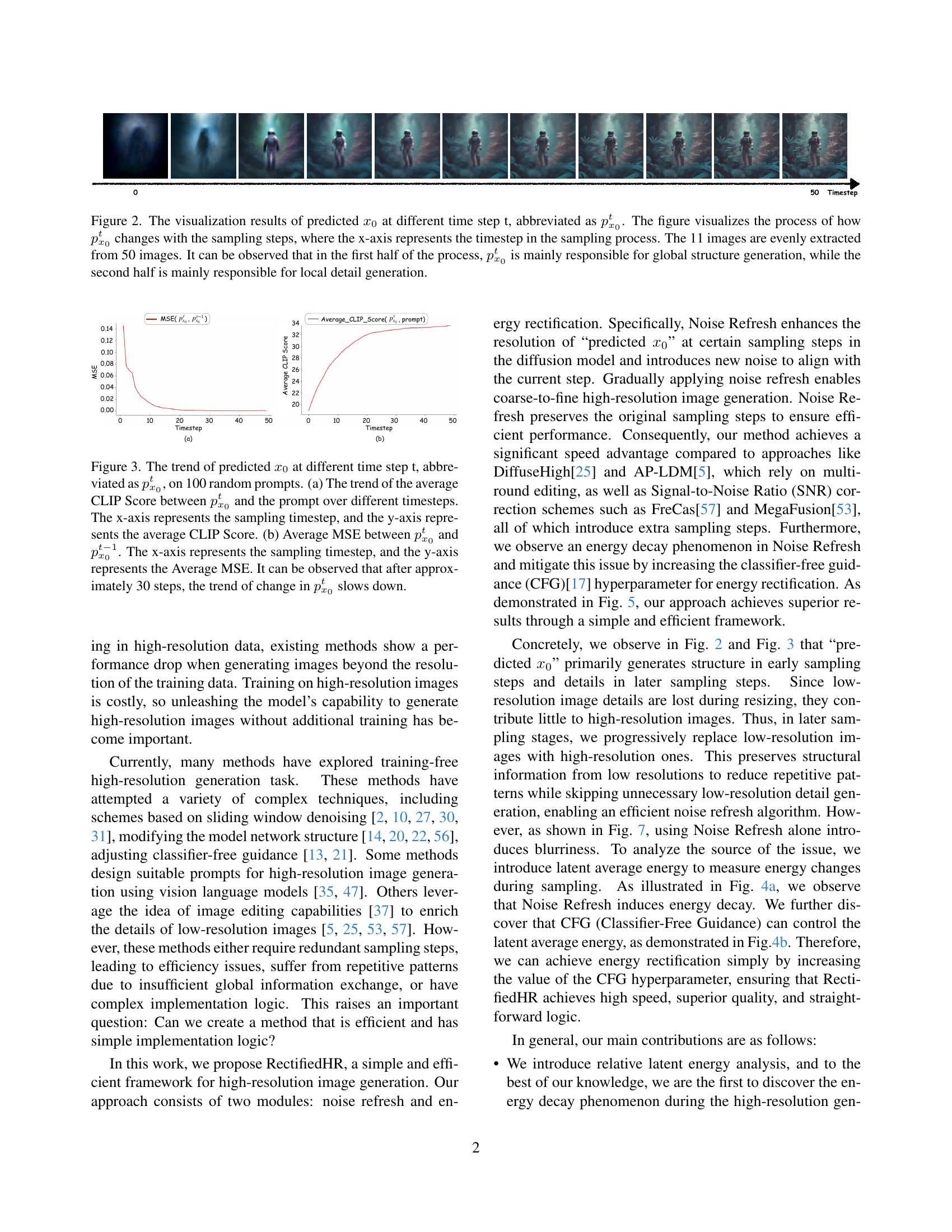
🔼 Figure 2 visualizes the predicted x0 (denoted as p_x0^t) throughout the denoising process of a diffusion model. The x-axis represents the timestep, and the 11 displayed images are evenly sampled from the 50 timesteps. The figure demonstrates a transition in the generation process: during the first half, p_x0^t focuses on establishing the overall image structure; during the second half, it refines the details. This highlights the model’s two-stage approach to image generation.
read the caption
Figure 2: The visualization results of predicted x0subscript𝑥0x_{0}italic_x start_POSTSUBSCRIPT 0 end_POSTSUBSCRIPT at different time step t, abbreviated as px0tsuperscriptsubscript𝑝subscript𝑥0𝑡p_{x_{0}}^{t}italic_p start_POSTSUBSCRIPT italic_x start_POSTSUBSCRIPT 0 end_POSTSUBSCRIPT end_POSTSUBSCRIPT start_POSTSUPERSCRIPT italic_t end_POSTSUPERSCRIPT. The figure visualizes the process of how px0tsuperscriptsubscript𝑝subscript𝑥0𝑡p_{x_{0}}^{t}italic_p start_POSTSUBSCRIPT italic_x start_POSTSUBSCRIPT 0 end_POSTSUBSCRIPT end_POSTSUBSCRIPT start_POSTSUPERSCRIPT italic_t end_POSTSUPERSCRIPT changes with the sampling steps, where the x-axis represents the timestep in the sampling process. The 11 images are evenly extracted from 50 images. It can be observed that in the first half of the process, px0tsuperscriptsubscript𝑝subscript𝑥0𝑡p_{x_{0}}^{t}italic_p start_POSTSUBSCRIPT italic_x start_POSTSUBSCRIPT 0 end_POSTSUBSCRIPT end_POSTSUBSCRIPT start_POSTSUPERSCRIPT italic_t end_POSTSUPERSCRIPT is mainly responsible for global structure generation, while the second half is mainly responsible for local detail generation.

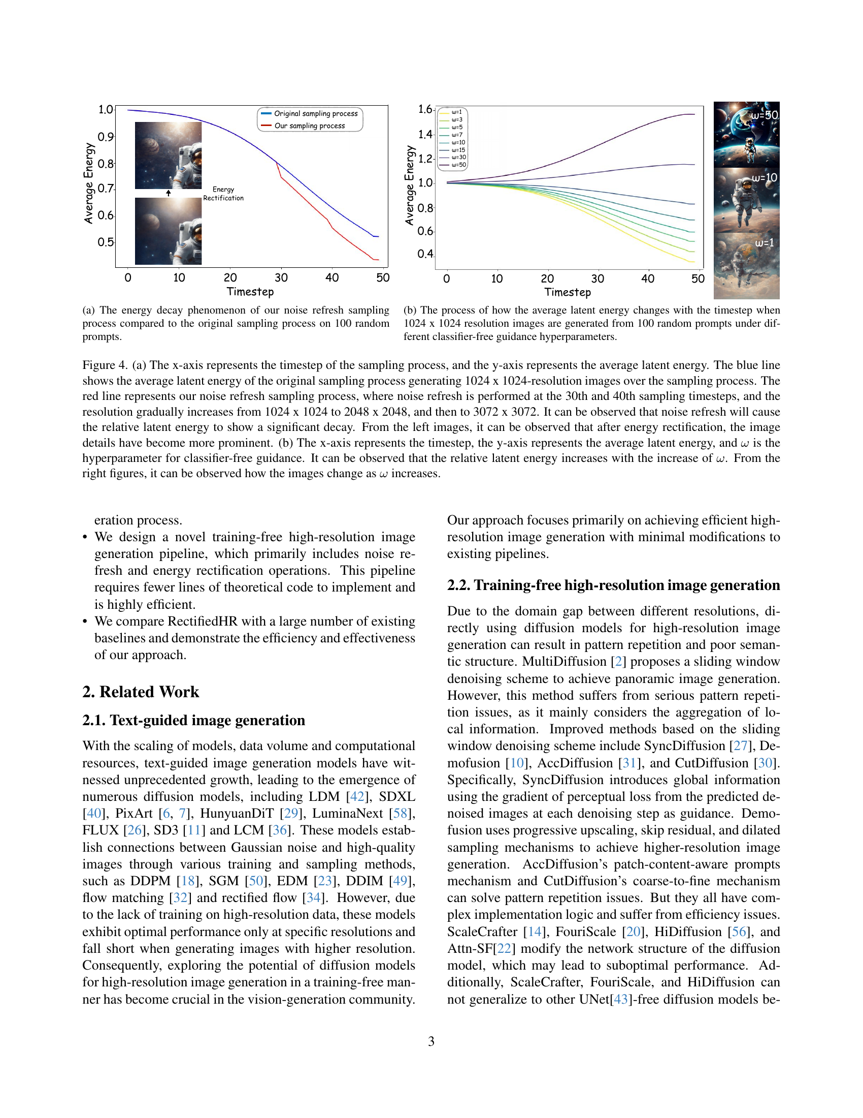
🔼 Figure 3 visualizes the change trends of predicted x0 (denoted as p_x₀^t) across different sampling timesteps (t) based on 100 random prompts. (a) shows the average CLIP score between p_x₀^t and the corresponding prompts, indicating how well the generated image matches the prompt at each timestep. (b) illustrates the average mean squared error (MSE) between p_x₀^t and p_x₀^t-1, showing the change in the generated image between consecutive steps. Both plots show a clear slowdown in the changes after approximately 30 sampling steps.
read the caption
Figure 3: The trend of predicted x0subscript𝑥0x_{0}italic_x start_POSTSUBSCRIPT 0 end_POSTSUBSCRIPT at different time step t, abbreviated as px0tsuperscriptsubscript𝑝subscript𝑥0𝑡p_{x_{0}}^{t}italic_p start_POSTSUBSCRIPT italic_x start_POSTSUBSCRIPT 0 end_POSTSUBSCRIPT end_POSTSUBSCRIPT start_POSTSUPERSCRIPT italic_t end_POSTSUPERSCRIPT, on 100 random prompts. (a) The trend of the average CLIP Score between px0tsuperscriptsubscript𝑝subscript𝑥0𝑡p_{x_{0}}^{t}italic_p start_POSTSUBSCRIPT italic_x start_POSTSUBSCRIPT 0 end_POSTSUBSCRIPT end_POSTSUBSCRIPT start_POSTSUPERSCRIPT italic_t end_POSTSUPERSCRIPT and the prompt over different timesteps. The x-axis represents the sampling timestep, and the y-axis represents the average CLIP Score. (b) Average MSE between px0tsuperscriptsubscript𝑝subscript𝑥0𝑡p_{x_{0}}^{t}italic_p start_POSTSUBSCRIPT italic_x start_POSTSUBSCRIPT 0 end_POSTSUBSCRIPT end_POSTSUBSCRIPT start_POSTSUPERSCRIPT italic_t end_POSTSUPERSCRIPT and px0t−1superscriptsubscript𝑝subscript𝑥0𝑡1p_{x_{0}}^{t-1}italic_p start_POSTSUBSCRIPT italic_x start_POSTSUBSCRIPT 0 end_POSTSUBSCRIPT end_POSTSUBSCRIPT start_POSTSUPERSCRIPT italic_t - 1 end_POSTSUPERSCRIPT. The x-axis represents the sampling timestep, and the y-axis represents the Average MSE. It can be observed that after approximately 30 steps, the trend of change in px0tsuperscriptsubscript𝑝subscript𝑥0𝑡p_{x_{0}}^{t}italic_p start_POSTSUBSCRIPT italic_x start_POSTSUBSCRIPT 0 end_POSTSUBSCRIPT end_POSTSUBSCRIPT start_POSTSUPERSCRIPT italic_t end_POSTSUPERSCRIPT slows down.

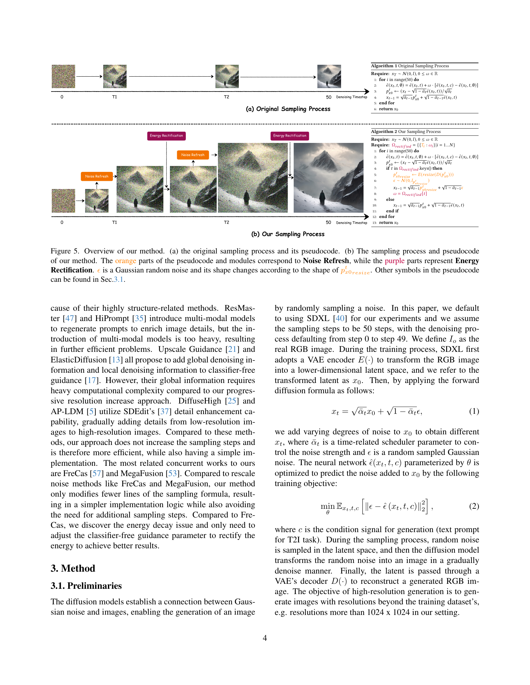
🔼 This figure compares the average latent energy over 50 sampling timesteps between the original sampling process and the proposed noise refresh sampling process. The original process shows a relatively stable energy level throughout sampling. In contrast, the noise refresh process shows a noticeable energy decay, especially after the 30th timestep, where noise refresh is applied. This decay is linked to image blurriness observed during high-resolution image generation. The images shown alongside the energy curves visually illustrate this effect, with a clearer image resulting from the less decayed energy level.
read the caption
(a) The energy decay phenomenon of our noise refresh sampling process compared to the original sampling process on 100 random prompts.

🔼 This figure shows how the average latent energy of an image changes over the sampling process of a diffusion model, specifically when generating 1024 x 1024 resolution images. The x-axis represents the timestep during the sampling process, and the y-axis shows the average latent energy. Multiple lines are plotted, each representing the average energy when using a different value for the classifier-free guidance (CFG) hyperparameter (w). The figure illustrates the impact of varying the CFG hyperparameter on the latent energy during the generation process. It demonstrates the effect of energy rectification on the latent energy. The right side shows how the changes in latent energy correlate with changes in generated image quality.
read the caption
(b) The process of how the average latent energy changes with the timestep when 1024 x 1024 resolution images are generated from 100 random prompts under different classifier-free guidance hyperparameters.

🔼 Figure 4 illustrates the impact of noise refresh and energy rectification on latent energy during the image generation process. (a) compares the average latent energy over sampling timesteps between the original process (generating 1024x1024 images) and the proposed method (noise refresh at steps 30 and 40, increasing resolution to 2048x2048 then 3072x3072). It highlights a significant energy decay caused by noise refresh, which is mitigated by energy rectification, leading to more detailed images, as shown in the accompanying image samples. (b) shows how average latent energy changes across sampling steps with varying classifier-free guidance (CFG) hyperparameters (ω). Higher CFG values correlate with increased energy and improved image quality, as demonstrated by the example images.
read the caption
Figure 4: (a) The x-axis represents the timestep of the sampling process, and the y-axis represents the average latent energy. The blue line shows the average latent energy of the original sampling process generating 1024 x 1024-resolution images over the sampling process. The red line represents our noise refresh sampling process, where noise refresh is performed at the 30th and 40th sampling timesteps, and the resolution gradually increases from 1024 x 1024 to 2048 x 2048, and then to 3072 x 3072. It can be observed that noise refresh will cause the relative latent energy to show a significant decay. From the left images, it can be observed that after energy rectification, the image details have become more prominent. (b) The x-axis represents the timestep, the y-axis represents the average latent energy, and ω𝜔\omegaitalic_ω is the hyperparameter for classifier-free guidance. It can be observed that the relative latent energy increases with the increase of ω𝜔\omegaitalic_ω. From the right figures, it can be observed how the images change as ω𝜔\omegaitalic_ω increases.

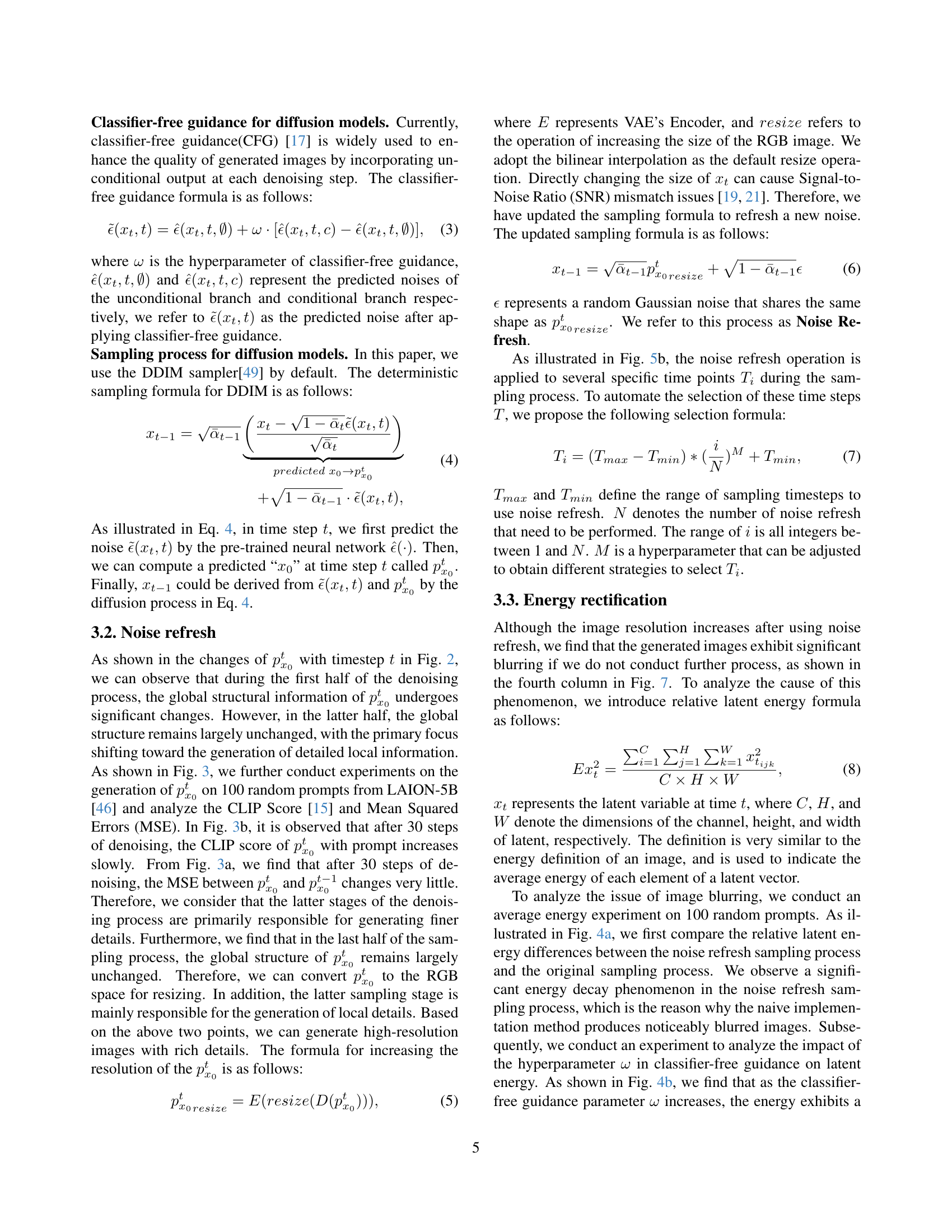
🔼 Figure 5 illustrates the core concept of the RectifiedHR method by comparing it to the original sampling process in a diffusion model. Panel (a) shows the original process, detailing how noise is gradually removed from a random noise sample to generate an image. The corresponding pseudocode is shown to the right. Panel (b) displays the RectifiedHR process which incorporates two key enhancements: Noise Refresh and Energy Rectification. The pseudocode in (b) highlights these additions in orange and purple, respectively. Noise Refresh improves resolution by resizing intermediate generated images (px0tresize). Energy Rectification adjusts the classifier-free guidance parameter (w) to correct energy decay observed during the high-resolution generation process, improving image clarity and reducing blurriness. The figure uses color-coding and pseudocode to make the improvements of the RectifiedHR approach easier to understand.
read the caption
Figure 5: Overview of our method. (a) the original sampling process and its pseudocode. (b) The sampling process and pseudocode of our method. The orange parts of the pseudocode and modules correspond to Noise Refresh, while the purple parts represent Energy Rectification. ϵitalic-ϵ{\color[rgb]{1,.5,0}\epsilon}italic_ϵ is a Gaussian random noise and its shape changes according to the shape of px⁢0tr⁢e⁢s⁢i⁢z⁢esubscriptsuperscriptsubscript𝑝𝑥0𝑡𝑟𝑒𝑠𝑖𝑧𝑒{\color[rgb]{1,.5,0}{p_{x0}^{t}}_{resize}}italic_p start_POSTSUBSCRIPT italic_x 0 end_POSTSUBSCRIPT start_POSTSUPERSCRIPT italic_t end_POSTSUPERSCRIPT start_POSTSUBSCRIPT italic_r italic_e italic_s italic_i italic_z italic_e end_POSTSUBSCRIPT. Other symbols in the pseudocode can be found in Sec.3.1.

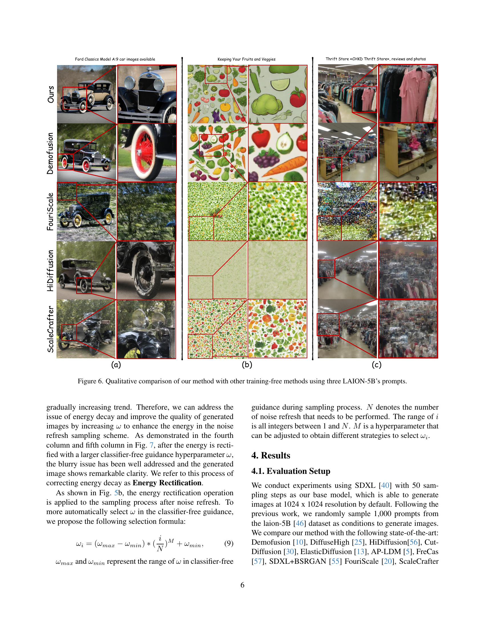
🔼 This figure presents a qualitative comparison of image generation results using different training-free high-resolution methods. Three distinct prompts from the LAION-5B dataset were used to generate images with each method: Ours (the proposed RectifiedHR method), FouriScale, ScaleCrafter, and DemoFusion and HiDiffusion. This allows for a visual assessment of the quality and characteristics of the images produced by each method, highlighting their strengths and weaknesses in terms of detail, structure, and artifacts.
read the caption
Figure 6: Qualitative comparison of our method with other training-free methods using three LAION-5B’s prompts.

TL;DR#

Key Takeaways#

Why does it matter?#

Visual Insights#

In-depth insights#

Energy Decay Info#

Noise Refresh#

RectifiedHR#

No Training HR#

Efficiency Boost#

More visual insights#

Full paper#