TL;DR#
Advancing AI in pathology demands extensive, high-quality datasets, yet current resources often lack diversity in organs, comprehensive class coverage, or sufficient annotation quality. To fill this gap, the authors introduce SPIDER (Supervised Pathology Image-DEscription Repository), the largest publicly available patch-level dataset. SPIDER encompasses Skin, Colorectal, and Thorax tissues with detailed class coverage. Expert pathologists verify annotations, enriching classification through spatial context using surrounding context patches.
SPIDER includes baseline models trained on the Hibou-L foundation model as a feature extractor, paired with an attention-based classification head, setting new performance standards across tissue types for digital pathology research. Beyond conventional patch classification, the model facilitates quick identification of key areas, calculates quantitative tissue metrics, and establishes a framework for multimodal strategies. Both the dataset and trained models are available publicly to facilitate research, ensure reproducibility, and promote AI-driven pathology development.
Key Takeaways#
Why does it matter?#
This paper introduces SPIDER, a large, multi-organ pathology dataset with expert annotations, crucial for advancing AI in digital pathology. It allows researchers to train more robust models, tackle diverse diagnostic tasks, and explore novel multimodal approaches for improved healthcare outcomes.
Visual Insights#

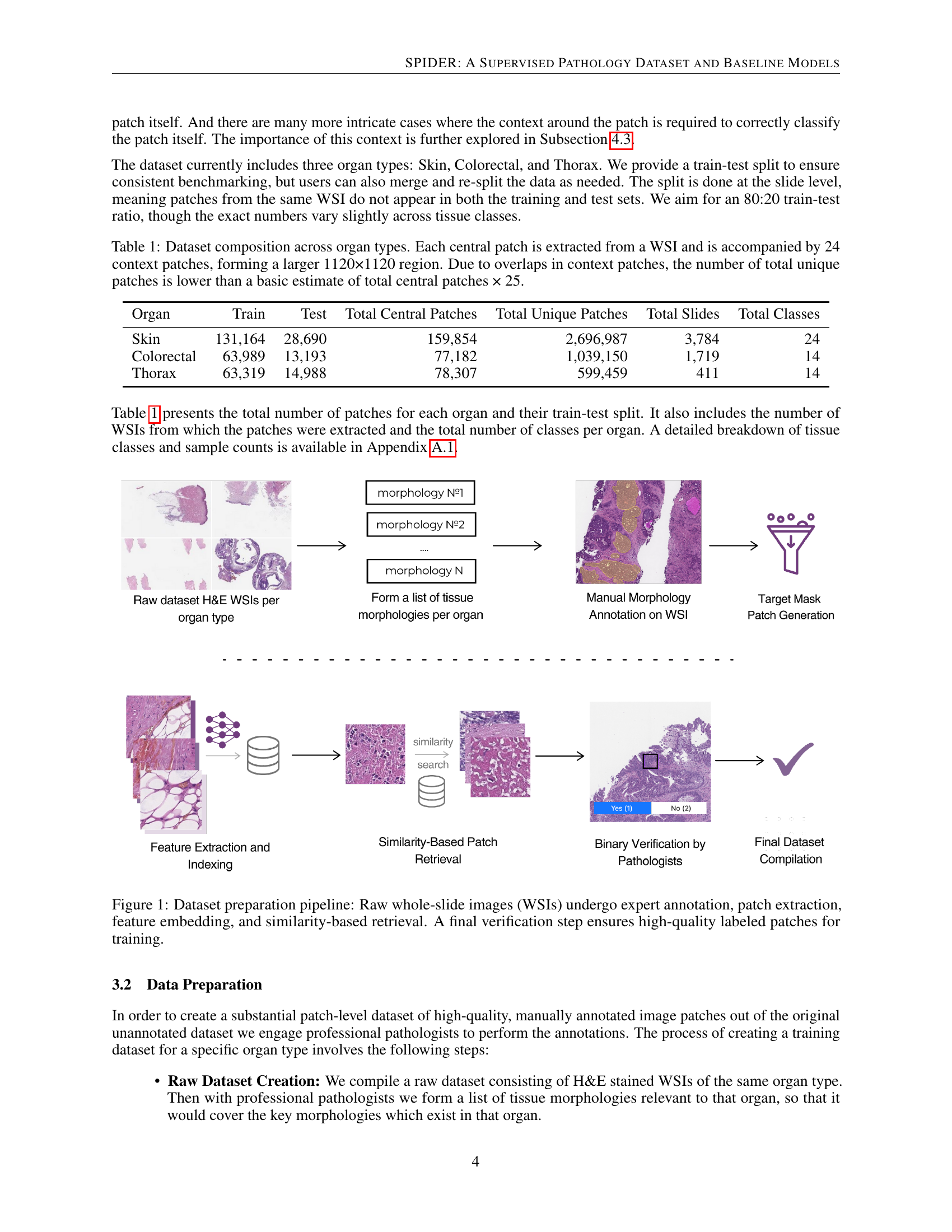
🔼 The figure illustrates the multi-step process of creating the SPIDER dataset. It begins with raw whole-slide images (WSIs) that are manually annotated by expert pathologists to identify regions of interest representing different tissue morphologies. These annotated WSIs then undergo patch extraction, where the images are divided into smaller, 224x224 pixel patches. Feature embedding is performed on these patches using the Hibou-L model. Then, a similarity-based retrieval method is used to identify additional visually similar patches from other WSIs, expanding the dataset size. Finally, all identified patches undergo a binary verification step by pathologists to guarantee high-quality labels, ensuring the patches are ready for model training. This entire process creates the high-quality dataset for the SPIDER project.
read the caption
Figure 1: Dataset preparation pipeline: Raw whole-slide images (WSIs) undergo expert annotation, patch extraction, feature embedding, and similarity-based retrieval. A final verification step ensures high-quality labeled patches for training.
| Organ | Train | Test | Total Central Patches | Total Unique Patches | Total Slides | Total Classes |
|---|---|---|---|---|---|---|
| Skin | 131,164 | 28,690 | 159,854 | 2,696,987 | 3,784 | 24 |
| Colorectal | 63,989 | 13,193 | 77,182 | 1,039,150 | 1,719 | 14 |
| Thorax | 63,319 | 14,988 | 78,307 | 599,459 | 411 | 14 |
🔼 Table 1 presents a detailed breakdown of the SPIDER dataset’s composition across three organ types: skin, colorectal, and thorax. It shows the number of training and testing patches for each organ type, along with the total number of central patches (224x224 pixels) extracted. Importantly, it highlights that each central patch is part of a larger 1120x1120 image region, including 24 surrounding context patches. Due to the overlap of these context patches, the total number of unique patches is less than a simple multiplication of the number of central patches by 25. Finally, the table indicates the total number of slides used for each organ and the number of unique classes represented in each organ.
read the caption
Table 1: Dataset composition across organ types. Each central patch is extracted from a WSI and is accompanied by 24 context patches, forming a larger 1120×1120 region. Due to overlaps in context patches, the number of total unique patches is lower than a basic estimate of total central patches × 25.
In-depth insights#
SPIDER Dataset#
The SPIDER dataset, as described in the paper, appears to be a significant contribution to the field of computational pathology. It addresses limitations present in existing datasets by offering a multi-organ, comprehensively annotated resource. A key feature is the high-quality, expert-verified annotations, which is crucial for reliable training of AI models. The inclusion of context patches alongside the central patch is a thoughtful design choice, recognizing the importance of spatial context in pathological diagnosis. The paper emphasizes the large scale and class coverage of SPIDER. The fact that the dataset was created from a private source, not included in training other existing models is an important design choice as it will now allow for benchmarking which will further spur innovation. The permissive open license will increase accessibility and accelerate research by a lot of the broader community.
Context Matters#
Context is crucial in histopathology image analysis. Isolated patches can be ambiguous, especially in distinguishing subtle tissue differences. Surrounding tissue structures provide valuable cues for accurate classification. Pathologists often assess tissue holistically, considering spatial relationships. Incorporating context, through methods like larger image windows or attention mechanisms, enhances diagnostic precision. Models that ignore context may misclassify tissue types due to lack of information from tissue interactions. Therefore, context-aware models are essential for emulating expert pathologist assessments. Furthermore, it improves tissue segmentation and supports the development of more clinically relevant insights. Ignoring context would result in limited and less reliable diagnostic interpretations.
Hibou Baseline#
The paper utilizes a Hibou-L foundation model as a core component for feature extraction. It is then combined with an attention-based classification head to classify pathology images. By freezing the Hibou feature extractor during training and focusing on training the classification head. This approach efficiently leverages the robust features learned during pretraining, allowing for strong performance even with a moderately sized dataset. This design reflects a deliberate choice to leverage the generalization capabilities of foundation models, mitigating overfitting and enhancing the model’s ability to perform well on diverse pathology images. This architecture serves as a strong baseline and starting point for future research.
Few Organs Now#
While the paper does not explicitly have a section titled ‘Few Organs Now,’ we can infer the implications of limited organ coverage in pathology datasets. Current datasets often focus on a single organ, hindering the development of generalizable AI models. This narrow focus means models trained on, say, colorectal tissue, may perform poorly on skin or lung tissue. The lack of organ diversity limits the scope of AI applications in computational pathology. Expanding datasets to include more organ types would enable the creation of more versatile and robust AI tools applicable across a broader range of diagnostic scenarios and research questions, ultimately improving diagnostic accuracy and efficiency for a wider patient population. SPIDER aims to tackle this limitation.
Supervised > VLM#
The text refers to ‘Supervised > VLM’, implying a transition or evolution from supervised learning methodologies towards Vision-Language Models (VLMs). This suggests leveraging the strengths of supervised learning, such as expert-annotated datasets for fine-tuning, to enhance VLM performance in computational pathology. The value lies in creating more detailed representations of tissue morphology and it helps to accelerate digital pathology research. Such models can be trained or augmented which require large amounts of paired text-image data and by automatically generating such pairs, the approach scales the development of richer AI solutions and it pushes the field towards more generalizable AI system.
More visual insights#
More on figures

🔼 This figure illustrates the architecture of the model used for patch-level classification in the SPIDER dataset. The model takes as input a large patch (1120x1120 pixels) composed of a central patch and 24 surrounding context patches. Each of these 25 smaller (224x224 pixels) patches is processed individually by the Hibou-L feature extractor. The resulting embeddings from all 25 patches are then concatenated and fed into a transformer-based classification head. This head utilizes an attention mechanism to weigh the importance of the central patch and its surrounding context patches. Finally, the classifier outputs probabilities for each class, which represent the likelihood of the central patch belonging to each class. The use of context patches is a key feature, designed to improve the accuracy of the central patch classification by providing additional spatial information.
read the caption
Figure 2: Model architecture overview: The classifier processes a central patch alongside surrounding context patches. Features are extracted using the Hibou-L model, and an attention-based classification head integrates context information to improve central patch classification.
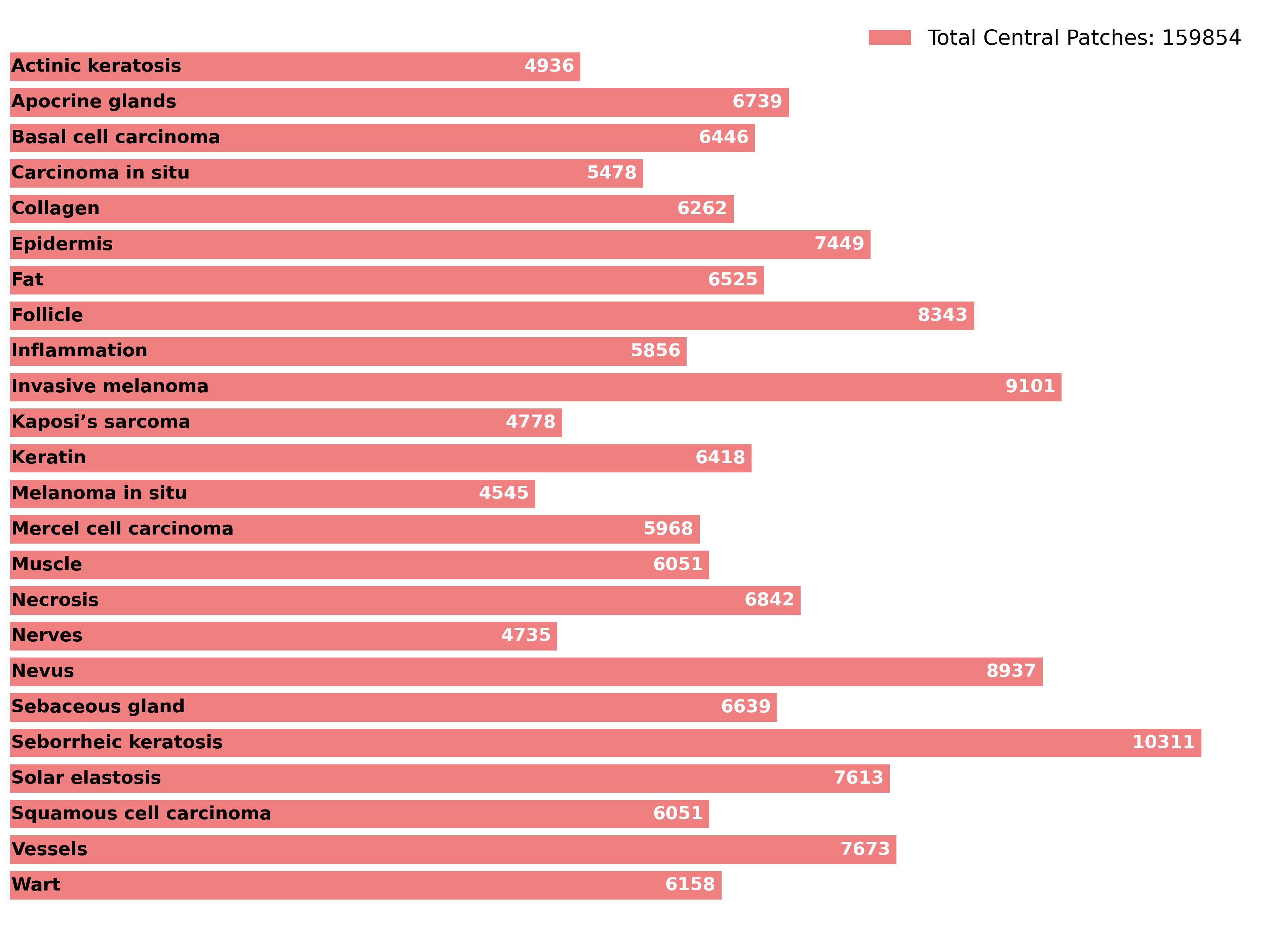
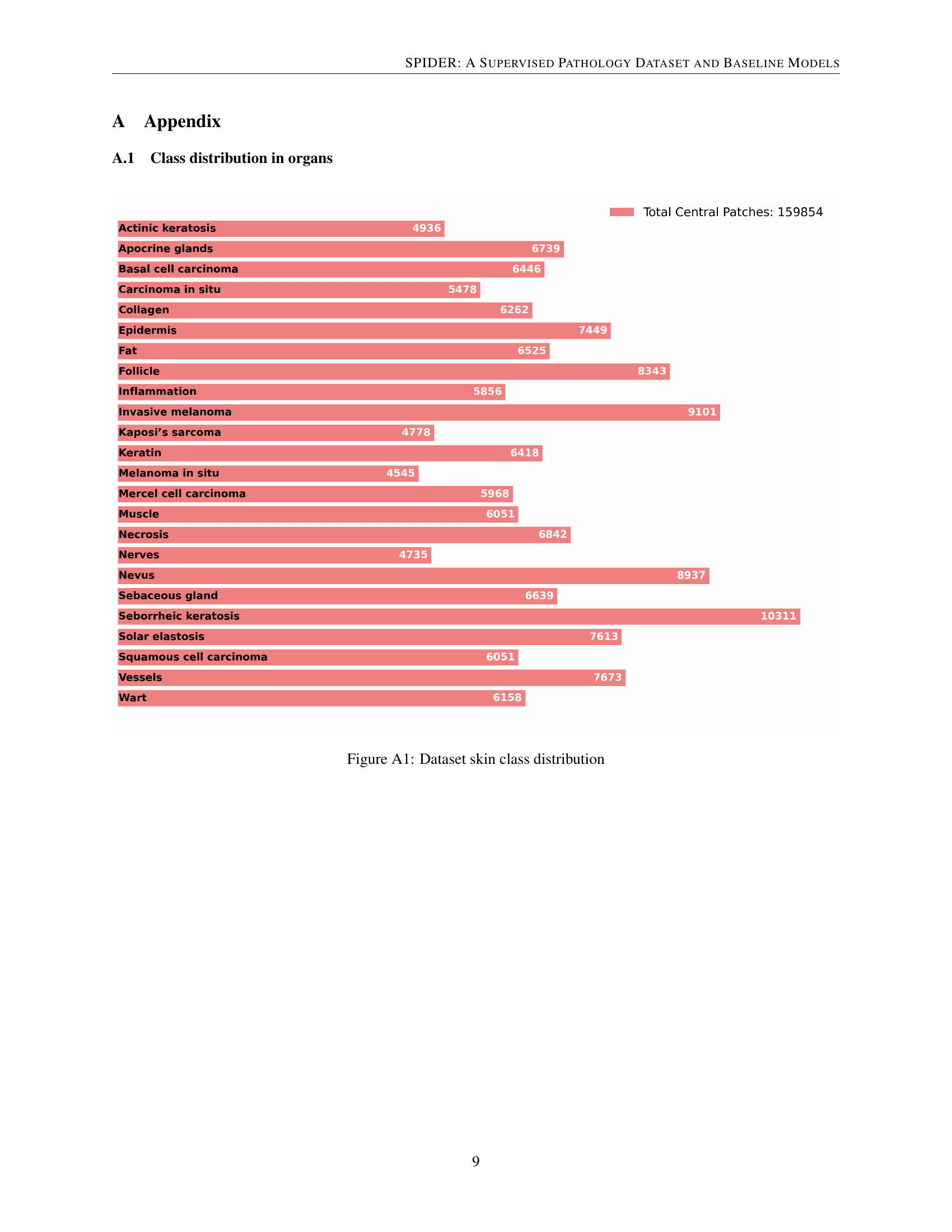
🔼 This bar chart visualizes the distribution of different skin tissue classes within the SPIDER dataset. Each bar represents a specific skin morphology (e.g., Actinic Keratosis, Basal Cell Carcinoma, Epidermis, etc.), and its length corresponds to the number of image patches belonging to that class. The total number of central patches in the dataset is also indicated.
read the caption
Figure A1: Dataset skin class distribution

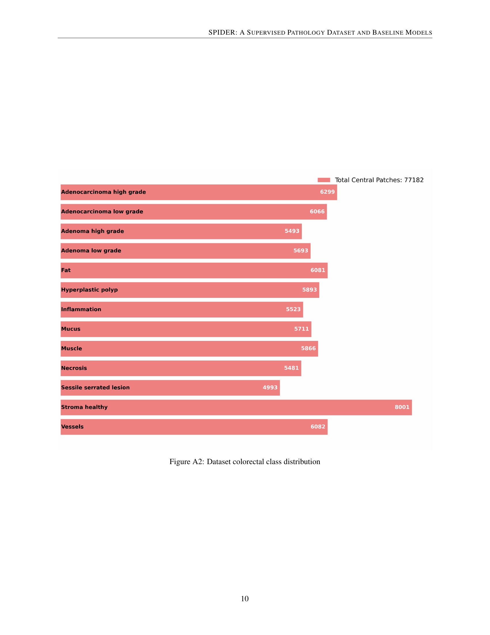
🔼 This bar chart visualizes the distribution of colorectal tissue classes within the SPIDER dataset. Each bar represents a specific colorectal tissue class (e.g., Adenocarcinoma High Grade, Adenoma Low Grade, etc.), and the length of the bar indicates the number of patches belonging to that class. The total number of central patches in the colorectal dataset is also displayed.
read the caption
Figure A2: Dataset colorectal class distribution

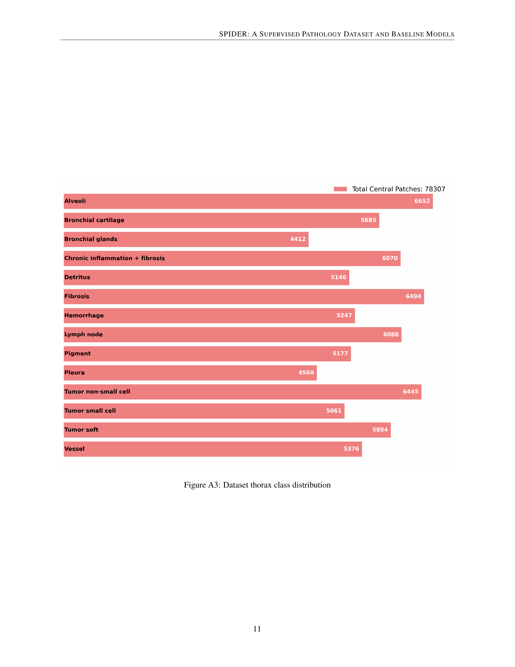
🔼 This bar chart visualizes the distribution of classes within the thorax section of the SPIDER dataset. Each bar represents a different tissue type (e.g., alveoli, bronchial glands, fibrosis, tumor) found in the thorax, and the length of the bar corresponds to the number of patches labeled with that specific class. The total number of central patches in the thorax dataset is also indicated in the legend.
read the caption
Figure A3: Dataset thorax class distribution

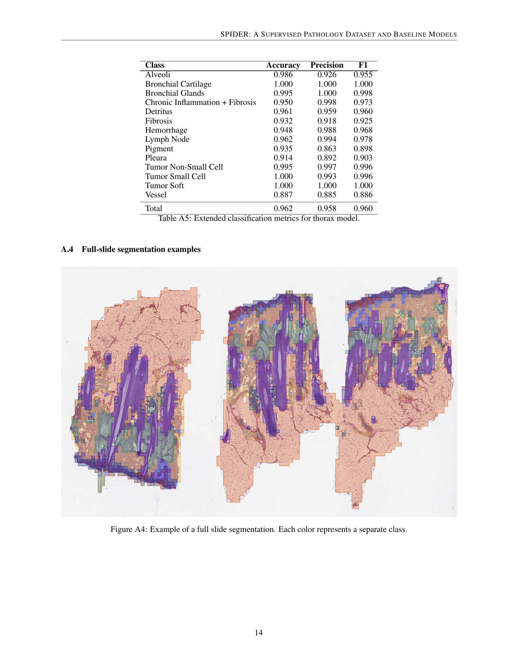
🔼 This figure shows an example of a whole-slide image (WSI) that has been segmented using the model described in the paper. Each color in the image represents a different tissue class or morphology as identified by the model. The segmentation highlights the model’s ability to delineate different tissue types within the WSI, demonstrating its potential for applications such as region of interest (ROI) identification and quantitative analysis of tissue composition.
read the caption
Figure A4: Example of a full slide segmentation. Each color represents a separate class.
More on tables
| Organ | Accuracy | Precision | F1 |
|---|---|---|---|
| Skin | 0.940 | 0.935 | 0.937 |
| Colorectal | 0.914 | 0.917 | 0.915 |
| Thorax | 0.962 | 0.958 | 0.960 |
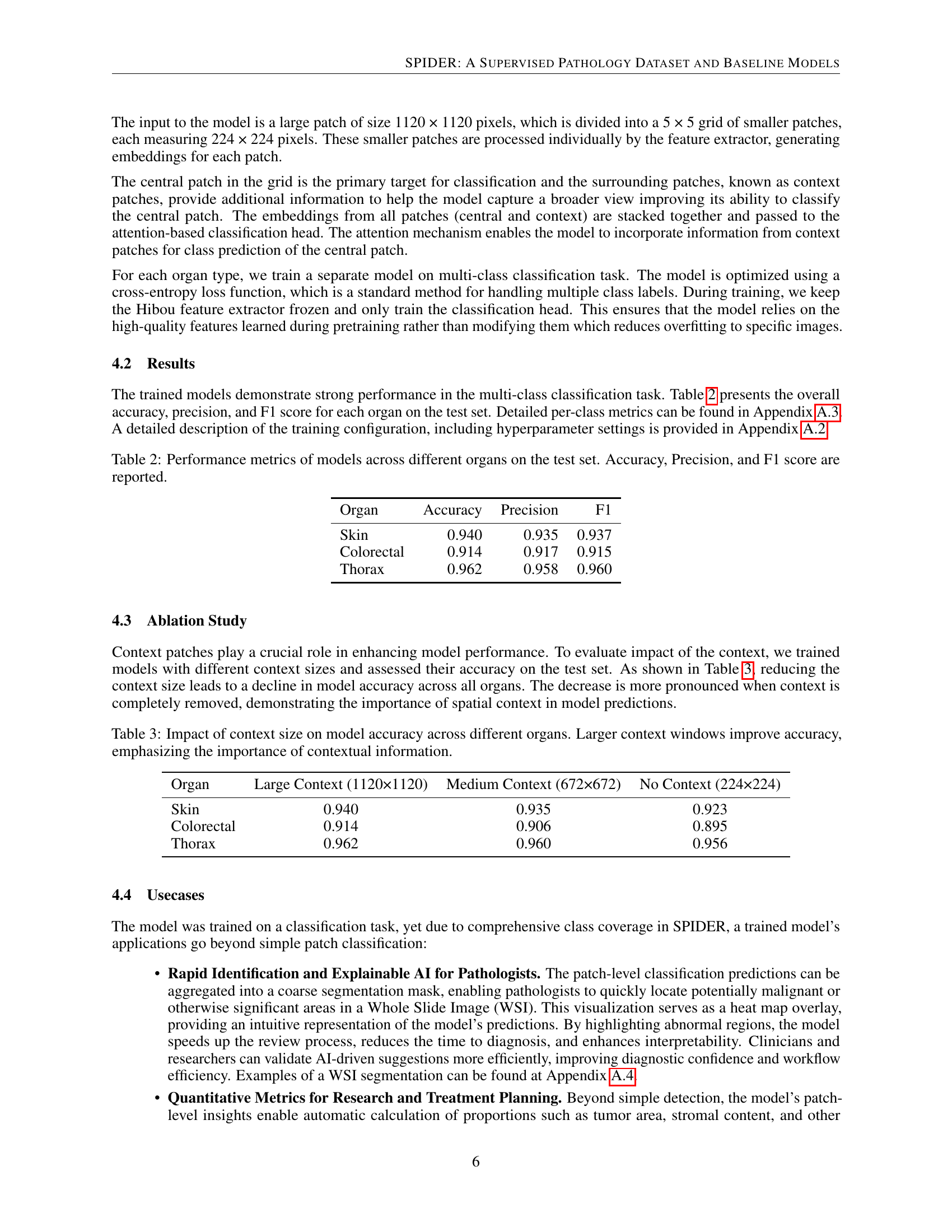
🔼 This table presents the performance of the trained models on the test dataset, broken down by organ (Skin, Colorectal, and Thorax). For each organ, the table reports three key metrics: Accuracy (the overall correctness of the model’s predictions), Precision (the proportion of correctly identified positive cases out of all cases identified as positive), and F1 score (the harmonic mean of precision and recall, providing a balanced measure of model performance). The F1 score is particularly useful when dealing with imbalanced datasets, as it considers both false positives and false negatives.
read the caption
Table 2: Performance metrics of models across different organs on the test set. Accuracy, Precision, and F1 score are reported.
| Organ | Large Context (1120×1120) | Medium Context (672×672) | No Context (224×224) |
|---|---|---|---|
| Skin | 0.940 | 0.935 | 0.923 |
| Colorectal | 0.914 | 0.906 | 0.895 |
| Thorax | 0.962 | 0.960 | 0.956 |
🔼 This table presents the results of an ablation study investigating the effect of different context window sizes on the model’s accuracy for classifying pathology images. Three different context sizes are evaluated: a large context (1120x1120 pixels), a medium context (672x672 pixels), and no context (224x224 pixels). The accuracy of the model is reported for each context size and for three different organs: Skin, Colorectal, and Thorax. The results demonstrate that larger context windows significantly improve the model’s accuracy, highlighting the importance of contextual information in accurate image classification.
read the caption
Table 3: Impact of context size on model accuracy across different organs. Larger context windows improve accuracy, emphasizing the importance of contextual information.
| Parameter | Value |
|---|---|
| Epochs | 10 |
| Batch size | 256 |
| Loss function | Cross entropy |
| Label smoothing | 0.2 |
| Optimizer | AdamW [14] |
| Learning rate | |
| Weight decay | 0.01 |
| Learning rate scheduler | Linear warmup + Cosine annealing |
| Warmup epochs | 1 |
| Mixed precision | FP16 |
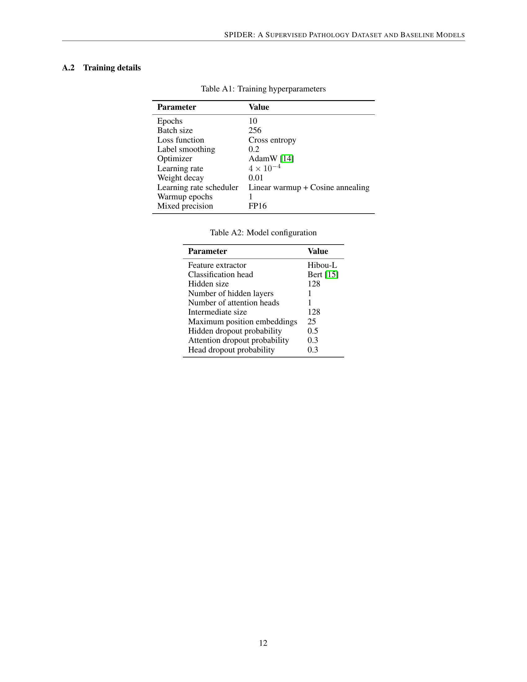
🔼 Table A1 presents the hyperparameters used during the training of the models. It details the settings for various aspects of the training process, including the number of training epochs, batch size, loss function used, label smoothing techniques, optimizer employed, learning rate, weight decay, and the learning rate scheduler strategy. The table also indicates the number of warmup epochs and the mixed precision used.
read the caption
Table A1: Training hyperparameters
| Parameter | Value |
| Feature extractor | Hibou-L |
| Classification head | Bert [15] |
| Hidden size | 128 |
| Number of hidden layers | 1 |
| Number of attention heads | 1 |
| Intermediate size | 128 |
| Maximum position embeddings | 25 |
| Hidden dropout probability | 0.5 |
| Attention dropout probability | 0.3 |
| Head dropout probability | 0.3 |
🔼 This table details the specific hyperparameters and architectural choices used to configure the model used in the experiments. It covers aspects of the feature extractor, classification head, and various layer dimensions, allowing for reproducibility and understanding of the model’s design.
read the caption
Table A2: Model configuration
| Class | Accuracy | Precision | F1 |
|---|---|---|---|
| Actinic Keratosis | 0.768 | 0.817 | 0.792 |
| Apocrine Glands | 0.999 | 0.999 | 0.999 |
| Basal Cell Carcinoma | 0.959 | 0.913 | 0.935 |
| Carcinoma In Situ | 0.761 | 0.698 | 0.728 |
| Collagen | 0.989 | 0.992 | 0.990 |
| Epidermis | 0.871 | 0.933 | 0.901 |
| Fat | 0.997 | 0.998 | 0.997 |
| Follicle | 0.942 | 0.953 | 0.947 |
| Inflammation | 0.926 | 0.974 | 0.949 |
| Invasive Melanoma | 0.936 | 0.937 | 0.937 |
| Kaposi’s Sarcoma | 0.990 | 0.906 | 0.946 |
| Keratin | 0.994 | 0.977 | 0.985 |
| Melanoma In Situ | 0.976 | 0.962 | 0.969 |
| Mercel Cell Carcinoma | 0.887 | 0.998 | 0.939 |
| Muscle | 0.984 | 0.984 | 0.984 |
| Necrosis | 0.981 | 0.954 | 0.967 |
| Nerves | 0.999 | 1.000 | 0.999 |
| Nevus | 0.973 | 0.981 | 0.977 |
| Sebaceous Gland | 0.987 | 0.984 | 0.985 |
| Seborrheic Keratosis | 0.929 | 0.914 | 0.922 |
| Solar Elastosis | 0.997 | 0.988 | 0.993 |
| Squamous Cell Carcinoma | 0.839 | 0.826 | 0.832 |
| Vessels | 0.991 | 0.991 | 0.991 |
| Wart | 0.881 | 0.772 | 0.823 |
| Total | 0.940 | 0.935 | 0.937 |
🔼 Table A3 presents a detailed breakdown of the model’s performance on the skin tissue classification task. For each skin morphology class (e.g., Actinic Keratosis, Apocrine Glands, Basal Cell Carcinoma, etc.), the table displays the accuracy, precision, and F1-score achieved by the model. These metrics provide a granular assessment of the model’s ability to correctly identify and classify each specific type of skin tissue, offering insights into the model’s strengths and weaknesses across different tissue classes.
read the caption
Table A3: Extended classification metrics for skin model.
| Class | Accuracy | Precision | F1 |
|---|---|---|---|
| Adenocarcinoma High Grade | 0.861 | 0.963 | 0.909 |
| Adenocarcinoma Low Grade | 0.819 | 0.848 | 0.833 |
| Adenoma High Grade | 0.805 | 0.762 | 0.783 |
| Adenoma Low Grade | 0.915 | 0.865 | 0.889 |
| Fat | 0.994 | 0.997 | 0.995 |
| Hyperplastic Polyp | 0.833 | 0.866 | 0.850 |
| Inflammation | 0.978 | 0.959 | 0.969 |
| Mucus | 0.895 | 0.818 | 0.855 |
| Muscle | 0.981 | 0.970 | 0.976 |
| Necrosis | 0.977 | 0.976 | 0.977 |
| Sessile Serrated Lesion | 0.889 | 0.961 | 0.924 |
| Stroma Healthy | 0.977 | 0.970 | 0.974 |
| Vessels | 0.961 | 0.969 | 0.965 |
| Total | 0.914 | 0.917 | 0.915 |
🔼 Table A4 presents a detailed breakdown of the model’s performance on a per-class basis for colorectal tissue classification. It shows the accuracy, precision, and F1 score achieved by the model for each specific colorectal tissue class in the test dataset. This provides a more granular view of the model’s capabilities than the overall accuracy reported in the main text, revealing strengths and weaknesses across various tissue types.
read the caption
Table A4: Extended classification metrics for colorectal model.
| Class | Accuracy | Precision | F1 |
|---|---|---|---|
| Alveoli | 0.986 | 0.926 | 0.955 |
| Bronchial Cartilage | 1.000 | 1.000 | 1.000 |
| Bronchial Glands | 0.995 | 1.000 | 0.998 |
| Chronic Inflammation + Fibrosis | 0.950 | 0.998 | 0.973 |
| Detritus | 0.961 | 0.959 | 0.960 |
| Fibrosis | 0.932 | 0.918 | 0.925 |
| Hemorrhage | 0.948 | 0.988 | 0.968 |
| Lymph Node | 0.962 | 0.994 | 0.978 |
| Pigment | 0.935 | 0.863 | 0.898 |
| Pleura | 0.914 | 0.892 | 0.903 |
| Tumor Non-Small Cell | 0.995 | 0.997 | 0.996 |
| Tumor Small Cell | 1.000 | 0.993 | 0.996 |
| Tumor Soft | 1.000 | 1.000 | 1.000 |
| Vessel | 0.887 | 0.885 | 0.886 |
| Total | 0.962 | 0.958 | 0.960 |
🔼 Table A5 presents a detailed breakdown of the model’s performance on the thorax organ dataset. It shows the accuracy, precision, and F1-score for each individual class within the thorax category, allowing for a granular assessment of the model’s strengths and weaknesses in classifying different thorax tissue types. This level of detail helps in understanding the overall model performance and identifying areas for potential improvement.
read the caption
Table A5: Extended classification metrics for thorax model.
Full paper#