TL;DR#
Serving LLMs is difficult due to their large size. Post-training quantization (PTQ) helps by compressing LLMs but relies on sensitivity metrics to identify important weights. Existing metrics are inaccurate due to the LLM’s complicated loss landscape. They underestimate the impact of quantization, as the quantized weights fall outside the convergence radius. Moreover, the sensitivity might change after quantization.
To solve these issues, this work introduces Post-quantization Integral (PQI), a new sensitivity metric that accurately estimates the influence of each quantized weight. PQI considers both original and quantized weights. The research also proposes ReQuant, a framework with two components: outlier selection and step-wise significant weights detach. Experiments show ReQuant improves PTQ, enhancing perplexity gain on Llama 3.2 1B with QTIP.
Key Takeaways#
Why does it matter?#
This paper is important because it introduces a novel approach to enhancing post-training quantization (PTQ) methods for LLMs. It can significantly boost the performance of existing PTQ techniques, making LLMs more accessible for deployment on resource-constrained devices and opening new research directions for quantization techniques.
Visual Insights#

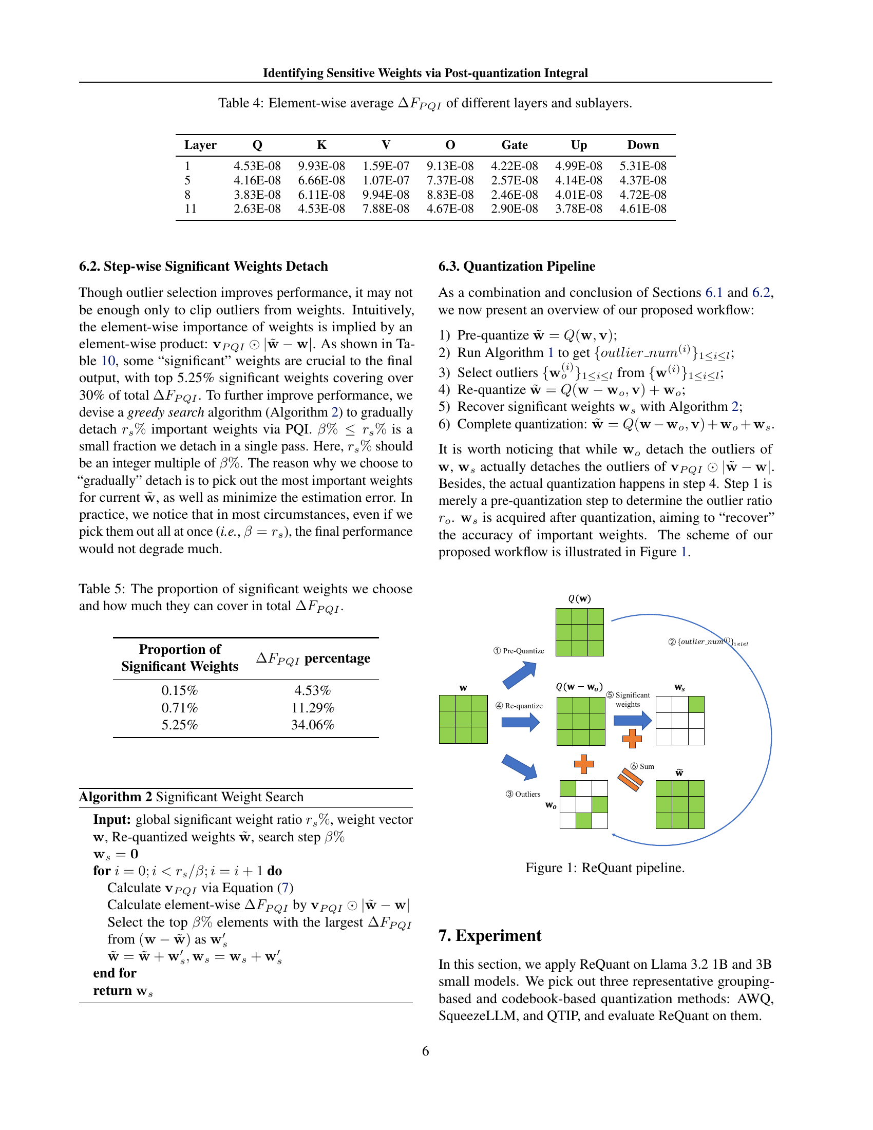
🔼 The ReQuant pipeline consists of six steps. First, the weights are pre-quantized using a traditional method and its sensitivity metric. Second, the optimal outlier ratio for each layer is determined using Algorithm 1. Third, outliers are selected based on this ratio. Fourth, the weights are re-quantized after removing the outliers. Fifth, significant weights are recovered using Algorithm 2. Finally, the low-precision dense weights, sparse outliers and significant weights are summed to form the final quantized weight.
read the caption
Figure 1: ReQuant pipeline.
| Quan- tized Layer | First-order | Second-order | Actual |
| 1 | 7.10E-04 | -5.98E-06 | 6.88E-03 |
| 2 | -6.58E-05 | -4.54E-06 | 4.45E-03 |
| 3 | -3.21E-04 | -3.66E-06 | 3.67E-03 |
| 4 | -5.04E-04 | -3.68E-06 | 3.82E-03 |
| 5 | -7.00E-04 | -3.75E-06 | 3.72E-03 |
| 6 | -6.29E-04 | -3.61E-06 | 4.27E-03 |
| 7 | -2.04E-04 | -3.63E-06 | 5.06E-03 |
| 8 | 6.82E-05 | -3.60E-06 | 5.59E-03 |
| 9 | 5.75E-05 | -3.97E-06 | 6.85E-03 |
| 10 | 2.86E-04 | -4.10E-06 | 7.78E-03 |
| 11 | -6.43E-04 | -3.66E-06 | 6.57E-03 |
| 12 | 8.29E-04 | -2.95E-06 | 6.81E-03 |
| 13 | 6.14E-04 | -2.80E-06 | 5.83E-03 |
| 14 | 1.30E-03 | -2.65E-06 | 6.57E-03 |
| 15 | -2.52E-04 | -2.84E-06 | 5.30E-03 |
| 16 | 3.47E-04 | -5.05E-06 | 9.79E-03 |
| All | 8.92E-04 | -6.05E-05 | 1.00E-01 |
🔼 Table 1 presents a detailed breakdown of the accuracy of first-order and second-order Taylor expansion approximations in predicting the actual change in loss function (ΔF) after weight quantization. It compares the calculated first-order and second-order terms from Equation 1 with the actual observed ΔF for each layer of a 16-layer Llama 3.2 1B language model. This comparison reveals the significant discrepancy between the approximation and reality, especially concerning the underestimation of the actual loss function change by orders of magnitude.
read the caption
Table 1: First-order, second-order term and actual ΔFΔ𝐹\Delta Froman_Δ italic_F in Equation 1.
In-depth insights#
PQI: Accuracy++#
While the title “PQI: Accuracy++” is speculative, it suggests a significant leap in accuracy attributable to the Post-quantization Integral (PQI). The “++” implies PQI isn’t merely an incremental improvement, but a substantial enhancement. This leap could stem from PQI’s ability to more accurately estimate the impact of quantization on individual weight dimensions, overcoming limitations of gradient/Hessian metrics. A central component of PQI’s accuracy is its fine-grained approach, estimating posterior sensitivity meticulously. It should also be noted that it can be combined with quantization methods. It is important to state that its accuracy lies in decomposing the path into numerous small fragments. As a result, Taylor’s formula can accurately approximate each fragment.
ReQuant: Key idea#
ReQuant introduces a novel approach to post-quantization by employing a Dense-and-Sparse detach strategy, which distinguishes it from traditional quantization methods. The core idea revolves around intelligently separating weights into dense, outlier, and significant components. The method first quantizes most of the weights using standard techniques (dense component), then preserves a small subset of outlier weights in high precision to mitigate accuracy loss. Critically, ReQuant identifies and detaches weights that, while not necessarily outliers, have a disproportionate impact on the model’s performance post-quantization (significant weights). By treating these crucial weights separately, ReQuant aims to strike a balance between aggressive compression and maintaining model fidelity. This allows for more effective quantization without sacrificing accuracy, as demonstrated by its performance improvements on LLMs.
Sparse Detach#
The sparse detach component is likely a crucial step in optimizing the quantization process for Large Language Models (LLMs). It probably involves selectively removing or isolating a subset of weights deemed less critical, or outliers, to improve overall model performance after quantization. This approach is based on the idea that not all weights contribute equally. By focusing quantization efforts on the most sensitive weights and detaching or handling outliers differently, the impact of reduced precision can be minimized. This is often achieved by maintaining a certain percentage of weights in higher precision. It is important as improper selection would degrade performance.
LLM Metric Flaws#
Existing metrics for evaluating weight quantization sensitivity in LLMs, such as gradient or Hessian-based approaches, suffer from inaccuracies. These metrics underestimate the impact of quantization on the loss function by orders of magnitude, mainly due to the small convergence radius of local second-order approximations. The complicated loss landscape of LLMs invalidates these approximations outside a tiny region around the original weights. Furthermore, the sensitivity calculated on original weights may not align with the actual sensitivity of quantized weights, as previously important weights may lose significance after quantization, and vice-versa, thus, these metrics fail to accurately predict the change in loss caused by weight quantization. Therefore, a new metric is needed.
Limited Radius#
The text discusses the convergence radius of Taylor’s expansion and how it affects the accuracy of sensitivity metrics used in post-training quantization (PTQ) for Large Language Models (LLMs). It argues that existing gradient and Hessian-based metrics are inaccurate due to the small convergence radius, meaning the local approximations they use are only valid in a very small region around the original weights. Quantization introduces significant changes, pushing the weights outside this radius. The Taylor series expansion becomes unreliable when the quantized weights fall outside the convergence radius of the original weights. The result is inaccurate estimation of the loss function change, hindering effective weight quantization.
More visual insights#
More on tables
| First-order | Second-order | Actual | |
| 1E-1 | 8.92E-5 | -6.05E-7 | 1.00E-3 |
| 5E-2 | 4.46E-5 | -1.51E-7 | 2.73E-4 |
| 1E-2 | 8.92E-6 | -6.05E-9 | 1.81E-5 |
| 5E-3 | 4.46E-6 | -1.51E-9 | 6.68E-6 |
| 1E-3 | 8.92E-7 | -6.05E-11 | 9.54E-7 |
🔼 This table shows how the accuracy of the Taylor expansion approximation for the change in loss function (ΔF) varies with different values of λ (lambda). λ controls how close the interpolated weight w’ is to the original weight w. As λ approaches 0, w’ gets closer to w, making the Taylor expansion more accurate. The table compares the actual change in loss (Actual ΔF) to the values predicted by the first-order and second-order terms of the Taylor expansion for various layers of a 16-layer Llama 3.2 1B model.
read the caption
Table 2: Actual ΔFΔ𝐹\Delta Froman_Δ italic_F with different λ𝜆\lambdaitalic_λ.
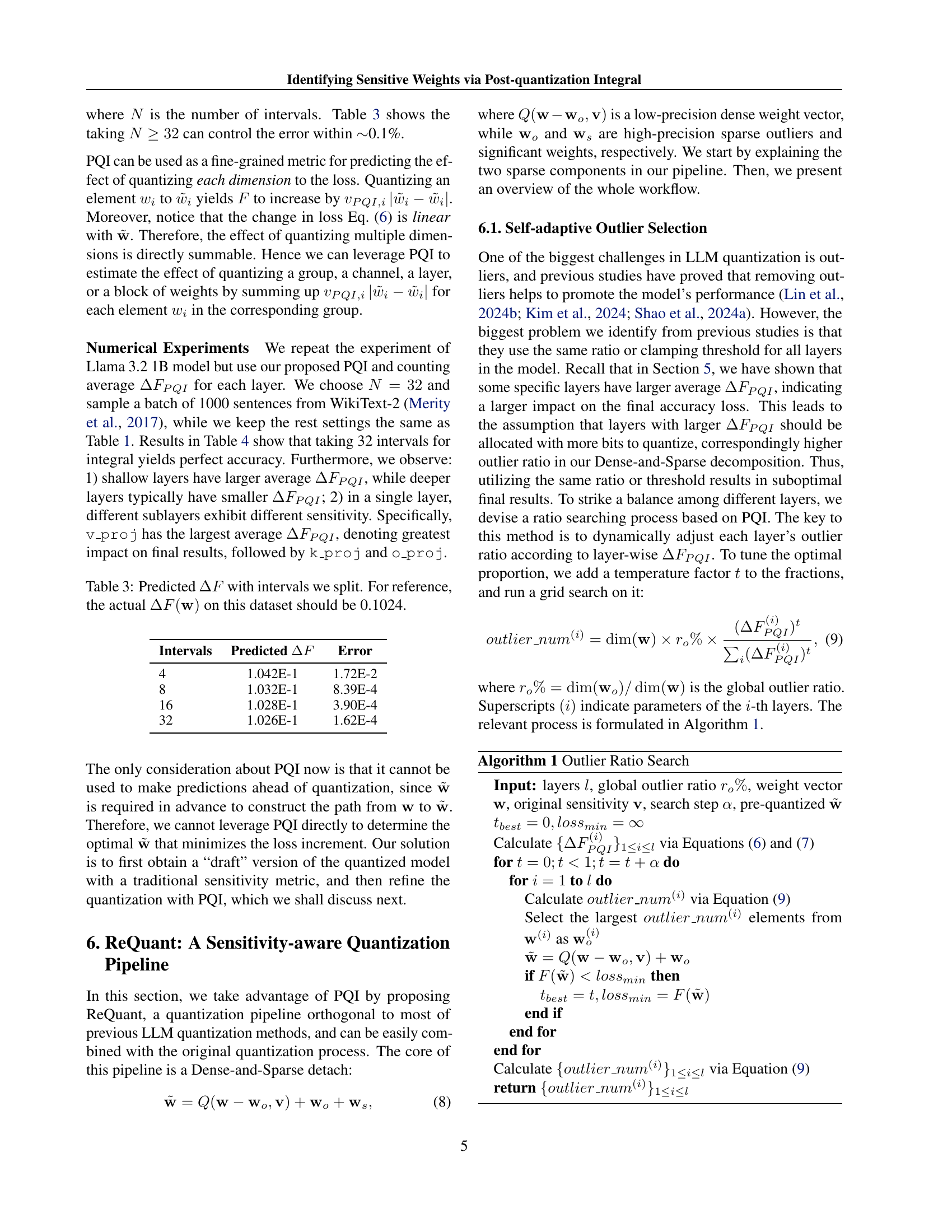
| Intervals | Predicted | Error |
| 4 | 1.042E-1 | 1.72E-2 |
| 8 | 1.032E-1 | 8.39E-4 |
| 16 | 1.028E-1 | 3.90E-4 |
| 32 | 1.026E-1 | 1.62E-4 |
🔼 This table presents the results of an experiment designed to evaluate the accuracy of the Post-quantization Integral (PQI) method, a novel sensitivity metric. The experiment quantifies the change in the loss function (ΔF) using PQI with varying numbers of intervals used in the numerical integration process. The goal is to demonstrate how well PQI can predict the actual change in the loss function. The actual ΔF for the dataset is provided for comparison, allowing assessment of PQI’s accuracy with different levels of granularity in the approximation.
read the caption
Table 3: Predicted ΔFΔ𝐹\Delta Froman_Δ italic_F with intervals we split. For reference, the actual ΔF(𝐰)Δ𝐹𝐰\Delta F(\bm{\mathbf{w}})roman_Δ italic_F ( bold_w ) on this dataset should be 0.1024.
| Layer | Q | K | V | O | Gate | Up | Down |
| 1 | 4.53E-08 | 9.93E-08 | 1.59E-07 | 9.13E-08 | 4.22E-08 | 4.99E-08 | 5.31E-08 |
| 5 | 4.16E-08 | 6.66E-08 | 1.07E-07 | 7.37E-08 | 2.57E-08 | 4.14E-08 | 4.37E-08 |
| 8 | 3.83E-08 | 6.11E-08 | 9.94E-08 | 8.83E-08 | 2.46E-08 | 4.01E-08 | 4.72E-08 |
| 11 | 2.63E-08 | 4.53E-08 | 7.88E-08 | 4.67E-08 | 2.90E-08 | 3.78E-08 | 4.61E-08 |
🔼 This table presents the element-wise average of the Post-quantization Integral (PQI) sensitivity metric for different layers and sub-layers within the Llama language model. The PQI metric quantifies the sensitivity of each weight to quantization, indicating its importance in maintaining model accuracy. Higher values suggest greater sensitivity and thus a larger impact on the model’s performance if that weight is quantized. The table helps to understand the varying sensitivity across different model components, informing strategies for more effective quantization.
read the caption
Table 4: Element-wise average ΔFPQIΔsubscript𝐹𝑃𝑄𝐼\Delta F_{PQI}roman_Δ italic_F start_POSTSUBSCRIPT italic_P italic_Q italic_I end_POSTSUBSCRIPT of different layers and sublayers.
| Proportion of Significant Weights | percentage |
| 0.15% | 4.53% |
| 0.71% | 11.29% |
| 5.25% | 34.06% |
🔼 This table shows the relationship between the percentage of weights considered ‘significant’ and their cumulative contribution to the total post-quantization integral (PQI) sensitivity metric. The PQI sensitivity metric quantifies how much each weight’s quantization affects the model’s loss. Higher ΔFPQI values indicate greater sensitivity. The table helps illustrate the impact of focusing on a smaller subset of most sensitive weights in the model’s quantization.
read the caption
Table 5: The proportion of significant weights we choose and how much they can cover in total ΔFPQIΔsubscript𝐹𝑃𝑄𝐼\Delta F_{PQI}roman_Δ italic_F start_POSTSUBSCRIPT italic_P italic_Q italic_I end_POSTSUBSCRIPT.
| Precision | Method | Calib Set | Sparsity | Bits | Mem | Base | Instruct | |
| (GB) | Wiki2 | MATH | ||||||
| full | Baseline | - | - | - | 16 | 2.30 | 9.75 | 29.30 |
| 2-bit | QTIP | RedPajama | - | - | 2.02 | 1.40 | 18.67 | 0.78 |
| QTIP+ReQuant | RedPajama/WikiText-2/Tulu 3 | 0 | 0.5 | 2.26 | 1.47 | 16.01 | 2.68 | |
| 3-bit | QTIP | RedPajama- | - | - | 3.02 | 1.72 | 11.17 | 18.78 |
| QTIP+ReQuant | RedPajama/WikiText-2/Tulu 3 | 0 | 0.5 | 3.26 | 1.80 | 10.83 | 20.06 | |
| 4-bit | QTIP | RedPajama | - | - | 4.02 | 2.05 | 10.12 | 26.38 |
| QTIP+ReQuant | RedPajama/WikiText-2/Tulu 3 | 0 | 0.5 | 4.26 | 2.13 | 10.06 | 27.36 | |
🔼 This table presents the results of applying the QTIP (Quantization with Trellises and Incoherence Processing) method to the Llama 3.2 1B Base and Instruct models. It shows the performance metrics achieved at different precision levels (2-bit, 3-bit, 4-bit), using various calibration sets, and with the addition of the ReQuant method. Metrics include perplexity on the WikiText-2 benchmark and the MATH score, indicating performance on mathematical reasoning tasks. Sparsity refers to the proportion of weights that are sparsely stored instead of being fully quantized.
read the caption
Table 6: QTIP results for Llama 3.2 1B Base/Instruct models. The entries share the same meaning as Table 7.
| Llama 3.2 1B Base/Instruct | Hyperparameters | 3-bit | 4-bit | ||||||||
| Method | Calib Set | Sparsity | Bits | Mem | Base | Instruct | Bits | Mem | Base | Instruct | |
| (GB) | Wiki2 | MATH | (GB) | Wiki2 | MATH | ||||||
| Baseline | - | - | - | 16 | 2.30 | 9.75 | 29.30 | 16 | 2.30 | 9.75 | 29.30 |
| AWQ (g128) | Pile | - | - | 3.25 | 0.86 | 16.74 | fail | 4.25 | 0.97 | 10.84 | 22.82 |
| AWQ (g256)+ReQuant | Pile | 0.25 | 0 | 3.25 | 0.86 | 15.36 | fail | 4.25 | 0.97 | 10.65 | 24.32 |
| SqueezeLLM | WikiText-2 | 0.45 | 0.05 | 3.25 | 0.86 | 13.86 | 11.28 | 4.25 | 0.97 | 10.51 | fail |
| SqueezeLLM+ReQuant | WikiText-2 | 0.45 | 0.05 | 3.25 | 0.86 | 13.30 | 14.18 | 4.25 | 0.97 | 10.43 | 24.74 |
🔼 This table presents the results of evaluating various quantization methods (AWQ, SqueezeLLM, and QTIP) on Llama language models (3.2B and 3B). It shows the WikiText-2 perplexity for base models and the 4-shot MATH (Mathematical Problem Solving) evaluation score for instruction following models. The table compares baseline performance with the results obtained after applying the proposed ReQuant method. ‘Fail’ indicates instances where the model’s output could not be properly parsed due to errors.
read the caption
Table 7: WikiText-2 perplexity for base models and 4-shot MATH evaluation for instruction following models. “Fail” means failure to parse model’s output due to garbled characters.
| Llama 3.2 3B Base/Instruct | Hyperparameters | 3-bit | 4-bit | ||||||||
| Method | Calib Set | Sparsity | Bits | Mem | Base | Instruct | Bits | Mem | Base | Instruct | |
| (GB) | Wiki2 | MATH | (GB) | Wiki2 | MATH | ||||||
| Baseline | - | - | - | 16 | 5.98 | 7.81 | 44.92 | 16 | 5.98 | 7.81 | 44.92 |
| AWQ (g128) | Pile | - | - | 3.25 | 1.80 | 10.30 | 29.64 | 4.25 | 2.13 | 8.22 | 42.88 |
| AWQ (g256)+ReQuant | Pile | 0.25 | 0 | 3.24 | 1.80 | 9.98 | 35.08 | 4.24 | 2.13 | 8.20 | 42.20 |
| SqueezeLLM | WikiText-2 | 0.45 | 0.05 | 3.24 | 1.80 | 9.39 | 33.80 | 4.24 | 2.13 | 8.12 | 43.06 |
| SqueezeLLM+ReQuant | WikiText-2 | 0.45 | 0.05 | 3.24 | 1.80 | 9.47 | 35.34 | 4.24 | 2.13 | 8.14 | 42.24 |
🔼 This table presents the ablation study results on the WikiText-2 dataset, focusing on the impact of outlier selection and significant weight detach on perplexity. It compares the performance of the proposed ReQuant method against baselines, evaluating different settings for outlier selection and gradual weight detachment. The ‘rand’ row provides a control, where outliers and significant weights are randomly selected, highlighting the effectiveness of the proposed selection strategy.
read the caption
Table 8: Ablation results on WikiText-2 perplexity. The “rand” line indicates that 𝐰osubscript𝐰𝑜\bm{\mathbf{w}}_{o}bold_w start_POSTSUBSCRIPT italic_o end_POSTSUBSCRIPT and 𝐰ssubscript𝐰𝑠\bm{\mathbf{w}}_{s}bold_w start_POSTSUBSCRIPT italic_s end_POSTSUBSCRIPT are picked out randomly from the weights.
| Comment | Train PPL | Test PPL | ||
| - | - | bfloat16 | 10.20 | 9.75 |
| 0.45 | 0.05 | 10.95 | 10.45 | |
| 0.45 | 0 | 11.02 | 10.52 | |
| 0.45 | 0 | SqueezeLLM | 11.15 | 10.62 |
| 0 | 0.05 | 11.15 | 10.65 | |
| 0 | 0 | 11.30 | 10.80 | |
| 0.45 | 0.05 | rand | 11.28 | 10.77 |
| 0.45 | 0.05 | 10.94 | 10.42 | |
| 0.45 | 0.05 | 10.94 | 10.42 | |
| 0.45 | 0.05 | 10.95 | 10.45 |
🔼 This table presents the inference speed comparison between different quantization methods with and without the proposed ReQuant technique. It shows the time taken for pre-filling (preparing data), decoding (processing the data), and the total inference time for various model sizes and precision levels. The results are useful for assessing the performance impact of ReQuant on inference speed and for understanding the tradeoff between accuracy and speed.
read the caption
Table 9: Inference speed of Dense-and-Sparse decomposition.
| Model | Precision | Method | Prefilling | Decoding | Total |
| (ms) | (ms) | (ms) | |||
| 1B | 4-bit | AWQ | 13 | 23768 | 23781 |
| 1B | 4-bit | AWQ+PQI | 18 | 35204 | 35222 |
| 1B | 4-bit | SqueezeLLM | 86 | 47151 | 47237 |
| 1B | 4-bit | SqueezeLLM+ReQuant | 29 | 45266 | 45295 |
| 1B | 3-bit | SqueezeLLM | 85 | 33657 | 33742 |
| 1B | 3-bit | SqueezeLLM+ReQuant | 86 | 32568 | 32654 |
| 3B | 4-bit | AWQ | 31 | 59631 | 59662 |
| 3B | 4-bit | AWQ+ReQuant | 31 | 59174 | 59205 |
| 3B | 4-bit | SqueezeLLM | 230 | 56882 | 57112 |
| 3B | 4-bit | SqueezeLLM+ReQuant | 68 | 56372 | 56440 |
| 3B | 3-bit | SqueezeLLM | 229 | 56343 | 56572 |
| 3B | 3-bit | SqueezeLLM+ReQuant | 229 | 54640 | 54869 |
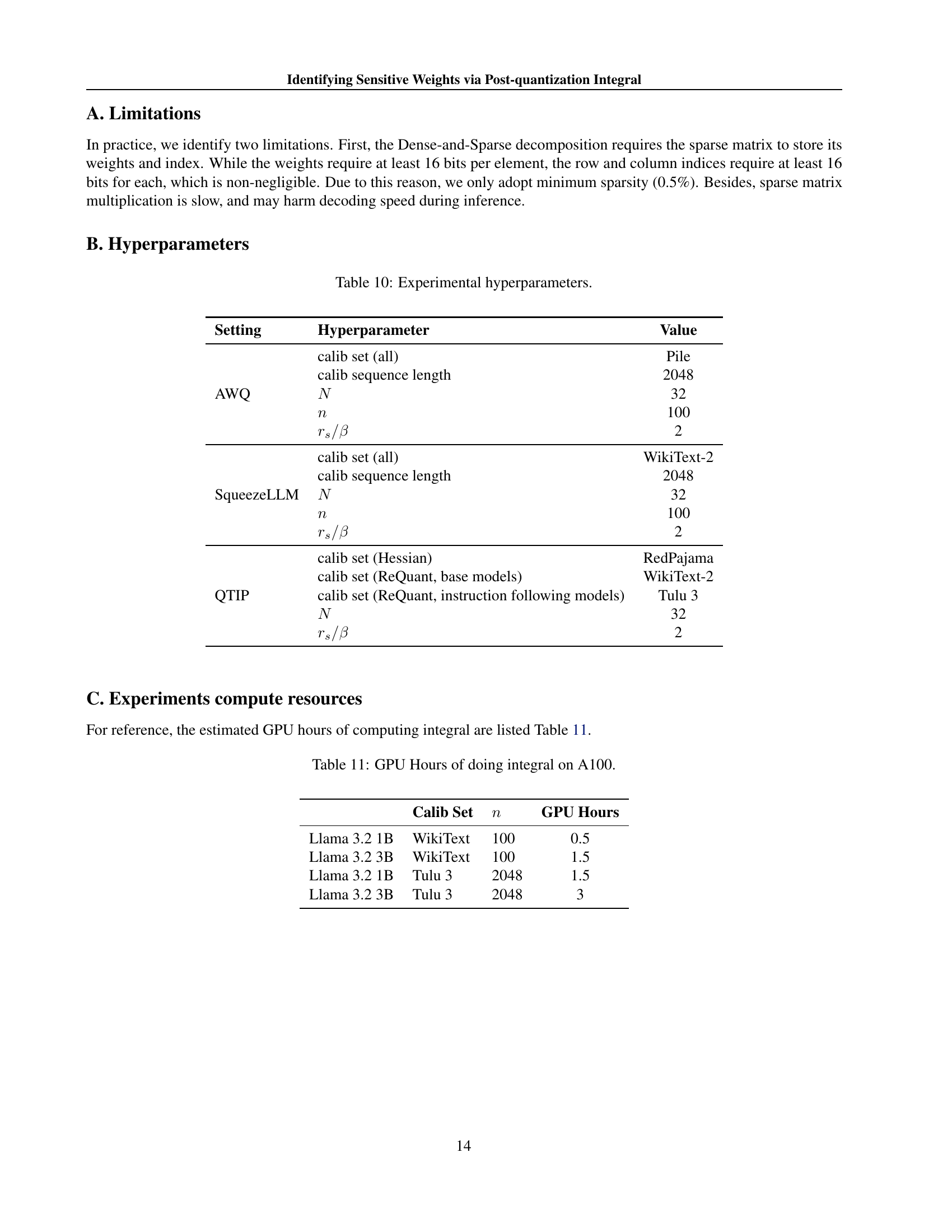
🔼 This table lists the hyperparameters used in the experiments for three different post-training quantization methods: AWQ, SqueezeLLM, and QTIP. For each method, it specifies the calibration dataset used, the sequence length of the calibration data, the number of intervals (N) used for the numerical integration in PQI, and the number of times (n) the dataset was sampled for calculations. It also gives the parameters rs and β used in the ReQuant method, representing the percentage of weights detached and the step size for that detachment respectively.
read the caption
Table 10: Experimental hyperparameters.
| Setting | Hyperparameter | Value |
| AWQ | calib set (all) | Pile |
| calib sequence length | 2048 | |
| 32 | ||
| 100 | ||
| 2 | ||
| SqueezeLLM | calib set (all) | WikiText-2 |
| calib sequence length | 2048 | |
| 32 | ||
| 100 | ||
| 2 | ||
| QTIP | calib set (Hessian) | RedPajama |
| calib set (ReQuant, base models) | WikiText-2 | |
| calib set (ReQuant, instruction following models) | Tulu 3 | |
| 32 | ||
| 2 |
🔼 This table shows the estimated GPU time (in hours) required for calculating the Post-quantization Integral (PQI) on an A100 GPU. It details the computation time for different model sizes (Llama 3.2 1B and 3.2 3B) and calibration datasets (WikiText-2 and Tulu 3) with varying numbers of samples (n). The size of the dataset used to calculate PQI significantly impacts the computational cost.
read the caption
Table 11: GPU Hours of doing integral on A100.
Full paper#