↗ arXiv ↗ Hugging Face ↗ Papers with Code
TL;DR#
Predicting the remaining lifespan of lithium-ion batteries (SOH prediction) is crucial for safe and efficient battery management. Current methods often struggle with the complexity and variability of real-world battery data. This paper introduces SambaMixer, a state-of-the-art model designed to tackle these challenges. Traditional models are often complex or computationally expensive.
SambaMixer uses a novel approach based on Mamba state space models, known for their efficiency in processing long sequences of data. It includes innovative resampling techniques to standardize the length of time series data and positional encoding to leverage additional time-related information (jitter, length differences). The results demonstrate that SambaMixer outperforms existing methods on the NASA battery dataset, showcasing its improved accuracy and robustness for SOH prediction. The open-sourced code makes it accessible to other researchers.
Key Takeaways#
Why does it matter?#
This paper is important because it presents SambaMixer, a novel and efficient model for predicting the state of health of lithium-ion batteries, a critical parameter for battery management systems. The model uses Mamba state space models, which are computationally efficient for handling long time series, and introduces novel resampling and positional encoding techniques. This improves accuracy and robustness, opening avenues for real-time, reliable battery health monitoring, critical for various applications. The open-sourced code further facilitates wider adoption and research.
Visual Insights#

🔼 This figure displays the impact of battery aging on voltage, current, and temperature measurements during multiple discharge cycles of a single lithium-ion battery. Specifically, it shows data from Battery #5 within the NASA battery dataset, which is a commonly used benchmark in battery research (Saha and Goebel, 2007). Each curve represents a different discharge cycle, illustrating how these signals change over time as the battery ages. You can observe the progressive degradation of the battery’s performance as the voltage decreases, current fluctuates, and temperature changes.
read the caption
Figure 1: Effect of battery aging on the measured voltage, current and temperature of various discharge cycles of a Li-ion battery. Battery #5 of NASA’s battery dataset (Saha and Goebel, 2007).
| Model | ||||
|---|---|---|---|---|
| SambaMixer-S | 256 | 16 | 8 | 4.7M |
| SambaMixer-M | 512 | 16 | 8 | 15.2M |
| SambaMixer-L | 768 | 24 | 12 | 48.7M |
| SambaMixer-XL | 1024 | 24 | 12 | 85.6M |
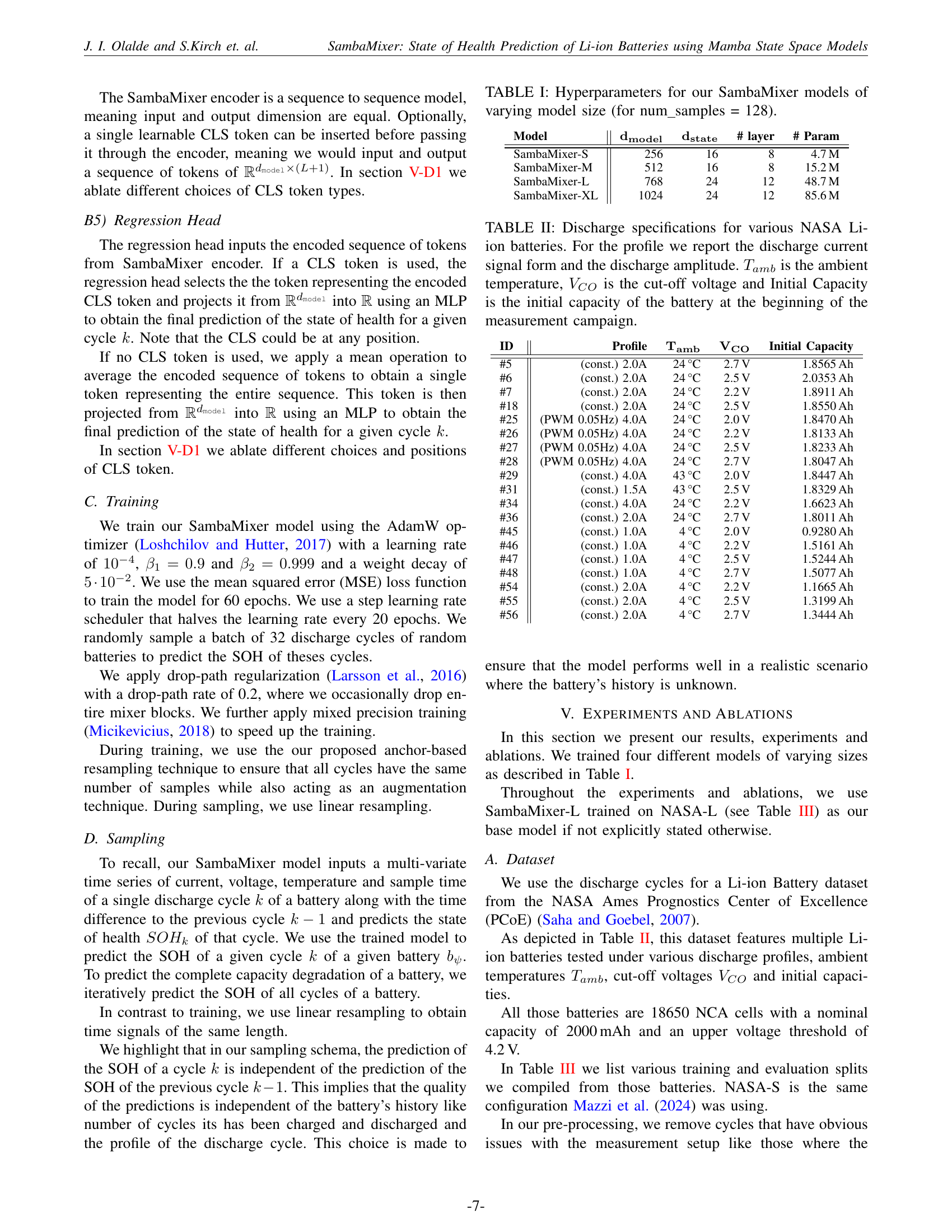
🔼 This table presents the hyperparameters used to configure different variations of the SambaMixer model. The models vary in size, which is reflected in the number of parameters, embedding dimension (dmodel), the dimension of the state space (dstate), the number of layers, and the total number of parameters in the model. The constant ’num_samples’ is set at 128 for all model configurations shown in the table.
read the caption
TABLE I: Hyperparameters for our SambaMixer models of varying model size (for num_samples = 128).
In-depth insights#
Mamba SSM for SOH#
The research paper introduces SambaMixer, a novel structured state space model (SSM) for Li-ion battery State of Health (SOH) prediction. Central to SambaMixer is the Mamba SSM architecture, which excels at handling multi-variate time series data inherent in battery monitoring. Unlike transformers, Mamba SSMs offer sub-quadratic time complexity, making them more efficient for long sequences. The paper further details an innovative anchor-based resampling technique to standardize time series lengths, acting as data augmentation. Positional encodings, incorporating sample time and cycle time differences, enhance accuracy by capturing recuperation effects. Experimental results on the NASA battery dataset demonstrate that SambaMixer significantly outperforms existing state-of-the-art methods, showcasing its potential for robust and accurate real-time battery health monitoring.
Anchor Resampling#
The research paper introduces anchor-based resampling as a novel technique to address the variable length of Li-ion battery discharge cycle time series data. This method tackles the challenge of inconsistent sample numbers across cycles, caused by differing sampling rates and the shortening cycle lengths as batteries age. Instead of simple linear or random resampling, which can distort the time series’ inherent dynamics, anchor-based resampling uses a set of equidistant anchors derived from linear resampling. Random noise is then added to these anchors to create variations, acting as a data augmentation technique that ensures the final dataset contains consistent sample sizes while preserving the temporal properties of the original signals. This addresses the overfitting issue in model training that might occur when training on varying-length sequences. The resulting resampled dataset is uniform, facilitating the use of state-of-the-art structured state-space models for accurate state-of-health prediction.
Time Encoding Impact#
The research explores the effect of incorporating time information into the model’s architecture using positional encodings. A sample time positional encoding is employed to address the varying lengths of time series data and to account for different sample rates, enhancing model robustness. A cycle time difference positional encoding is added to capture recuperation effects, where a battery’s SOH improves when not in use. This dual approach aims to improve accuracy and generalization. The results demonstrate that utilizing time information leads to superior performance compared to methods without this feature, highlighting the significance of integrating temporal dynamics into SOH prediction models. The effectiveness of different resampling techniques is also examined to show that ensuring equal sample length across datasets enhances model reliability and accuracy, even with varying sample rates. Therefore, time encoding is a crucial factor for improving both accuracy and robustness of SOH prediction in Li-ion batteries.
SambaMixer Ablation#
The SambaMixer ablation study systematically investigates the model’s design choices. The core backbone comparison reveals SambaMixer’s superiority over the vanilla Mamba model, highlighting the effectiveness of its multi-variate time signal handling capabilities. Resampling technique ablation demonstrates that the proposed anchor-based method outperforms linear and random approaches, suggesting its data augmentation benefits. Finally, ablation of positional encoding confirms the importance of incorporating both sample time and cycle time difference for capturing temporal dependencies and recuperation effects, ultimately improving accuracy and robustness.
Future Research#
The authors outline several key areas for future research. Expanding the dataset to include diverse battery chemistries and broader operational conditions is crucial for improved model generalizability. They also aim to investigate the influence of different discharge profiles on model performance, optimizing hyperparameters and architectures for enhanced accuracy. A further focus involves exploring alternative model architectures and state-space models to potentially enhance predictive capabilities. Finally, they plan a systematic examination of the impact of different hyperparameters and discharge profiles to fine-tune the model for optimal results. This multifaceted approach reflects a commitment to refining and expanding the SambaMixer model beyond its current capabilities.
More visual insights#
More on figures

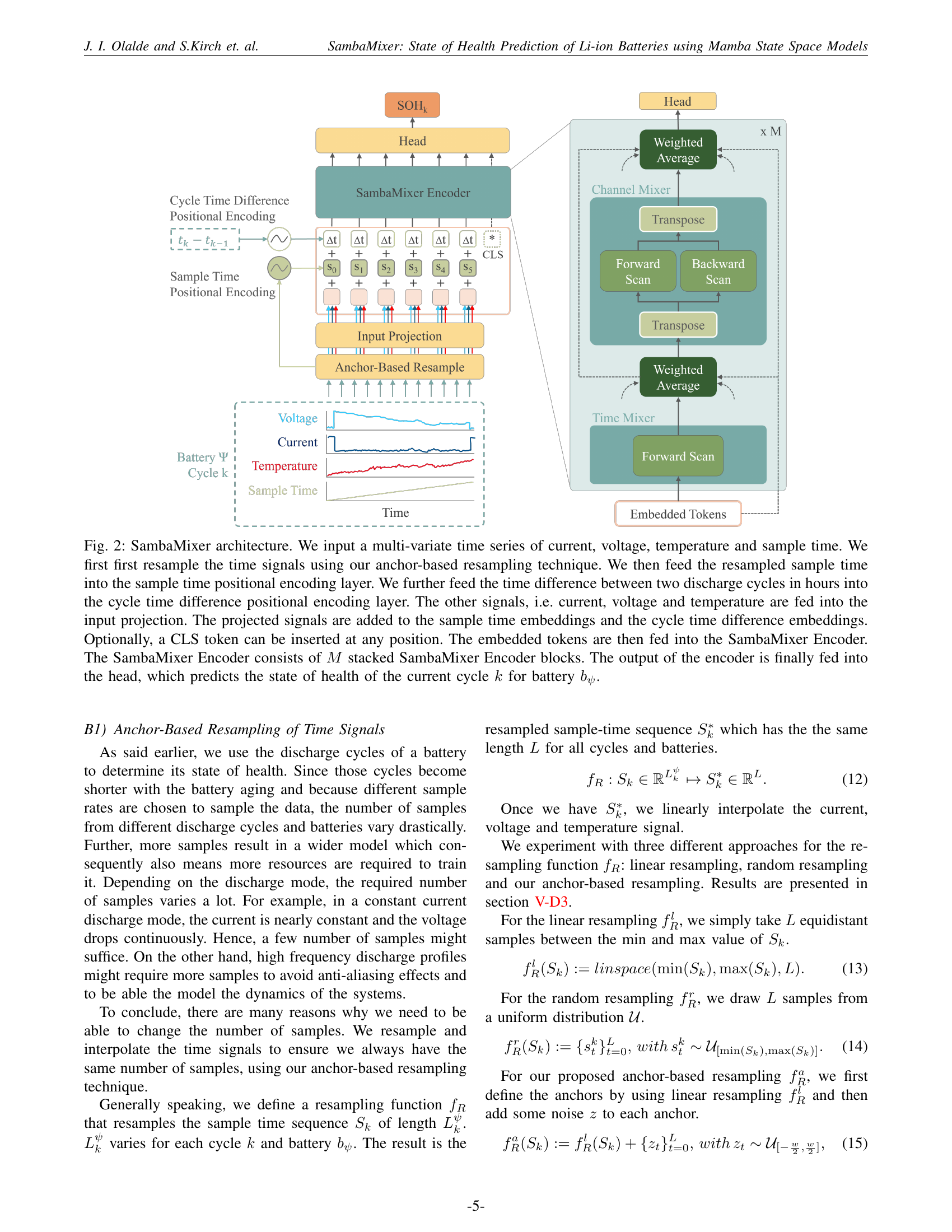
🔼 The SambaMixer architecture takes multi-variate time series data (current, voltage, temperature, and sample time) as input. The sample time is first resampled using an anchor-based method to ensure consistent length across different cycles. The resampled sample time is then fed into a positional encoding layer, along with the time difference between consecutive discharge cycles (in hours), which is also positionally encoded. The current, voltage, and temperature data undergoes an input projection layer before being combined with the positional embeddings. A CLS token (optional) can be added. This combined data feeds into the SambaMixer encoder, which consists of multiple stacked SambaMixer encoder blocks. The encoder output is finally passed to the head, which predicts the state of health (SOH) for a given cycle of a specific battery.
read the caption
Figure 2: SambaMixer architecture. We input a multi-variate time series of current, voltage, temperature and sample time. We first first resample the time signals using our anchor-based resampling technique. We then feed the resampled sample time into the sample time positional encoding layer. We further feed the time difference between two discharge cycles in hours into the cycle time difference positional encoding layer. The other signals, i.e. current, voltage and temperature are fed into the input projection. The projected signals are added to the sample time embeddings and the cycle time difference embeddings. Optionally, a CLS token can be inserted at any position. The embedded tokens are then fed into the SambaMixer Encoder. The SambaMixer Encoder consists of M𝑀Mitalic_M stacked SambaMixer Encoder blocks. The output of the encoder is finally fed into the head, which predicts the state of health of the current cycle k𝑘kitalic_k for battery bψsubscript𝑏𝜓b_{\psi}italic_b start_POSTSUBSCRIPT italic_ψ end_POSTSUBSCRIPT.

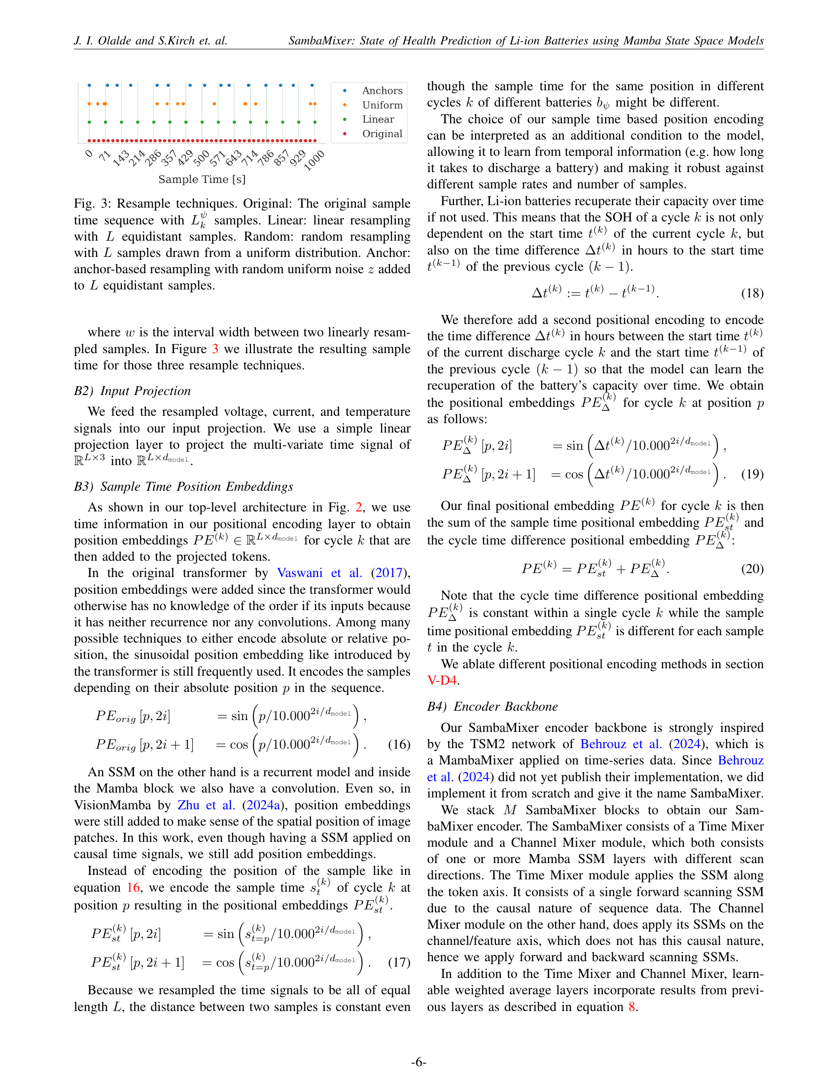
🔼 Figure 3 illustrates four different resampling techniques applied to a sample time sequence. The original sequence is shown with its actual, variable number of samples (represented as Lkψ). Three resampling methods are then compared to the original: linear resampling creates a new sequence with an equal number of equidistant samples; random resampling generates a new sequence with the same number of samples randomly selected from a uniform distribution across the range of the original data; finally, anchor-based resampling begins with equidistant samples (like linear resampling) but adds random noise to each sample, creating slight variations around the original equidistant anchors.
read the caption
Figure 3: Resample techniques. Original: The original sample time sequence with Lkψsuperscriptsubscript𝐿𝑘𝜓L_{k}^{\psi}italic_L start_POSTSUBSCRIPT italic_k end_POSTSUBSCRIPT start_POSTSUPERSCRIPT italic_ψ end_POSTSUPERSCRIPT samples. Linear: linear resampling with L𝐿Litalic_L equidistant samples. Random: random resampling with L𝐿Litalic_L samples drawn from a uniform distribution. Anchor: anchor-based resampling with random uniform noise z𝑧zitalic_z added to L𝐿Litalic_L equidistant samples.

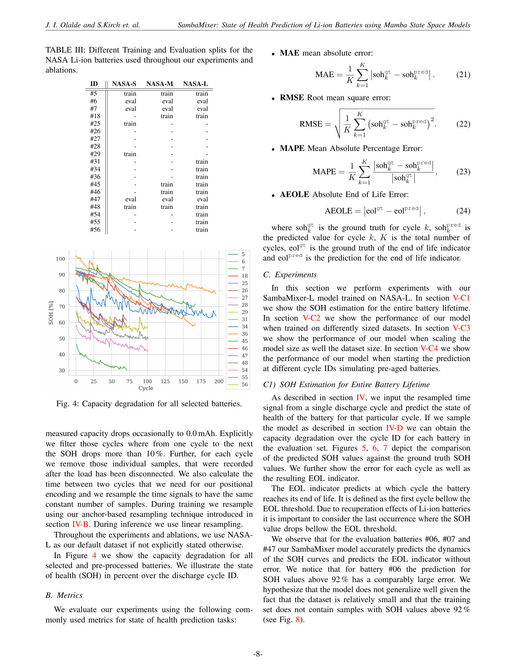
🔼 The figure visualizes the capacity degradation patterns observed across several lithium-ion batteries over their lifespan. The x-axis represents the cycle number (number of charge-discharge cycles), while the y-axis denotes the state of health (SOH) expressed as a percentage. Each line corresponds to a different battery, illustrating how the SOH diminishes over time. This graph highlights the variability in battery degradation rates and provides a visual representation of the data used to train and validate the models described in the paper.
read the caption
Figure 4: Capacity degradation for all selected batteries.

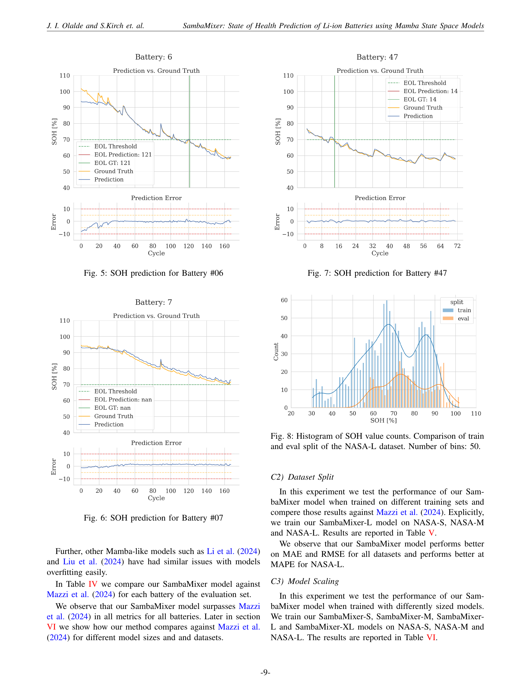
🔼 This figure displays the predicted state of health (SOH) for Battery #06 over its lifespan, alongside the actual measured SOH values. The plot showcases the model’s ability to accurately predict the battery’s degradation over time, with the predicted SOH values closely tracking the ground truth. It also shows the prediction error, highlighting the accuracy of the model’s predictions throughout the battery’s lifetime. Additionally, the plot indicates the predicted and actual end of life (EOL) of the battery, demonstrating the model’s capacity to foresee the point at which the battery reaches the end of its usable lifespan.
read the caption
Figure 5: SOH prediction for Battery #06

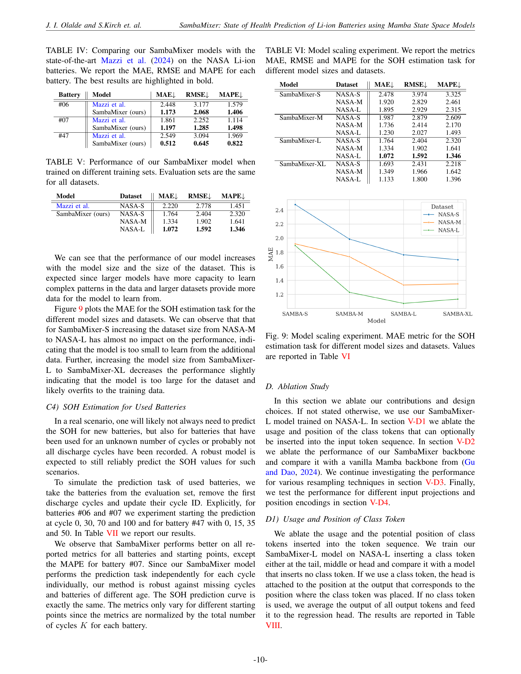
🔼 This figure showcases the predicted State of Health (SOH) values for Battery #07 over its lifespan, compared against the actual measured SOH. It provides a visual representation of the model’s accuracy in predicting SOH degradation over time, indicating both the predicted SOH and the prediction error. The plot also highlights the End of Life (EOL) prediction from the model and compares it to the actual EOL point for this specific battery.
read the caption
Figure 6: SOH prediction for Battery #07

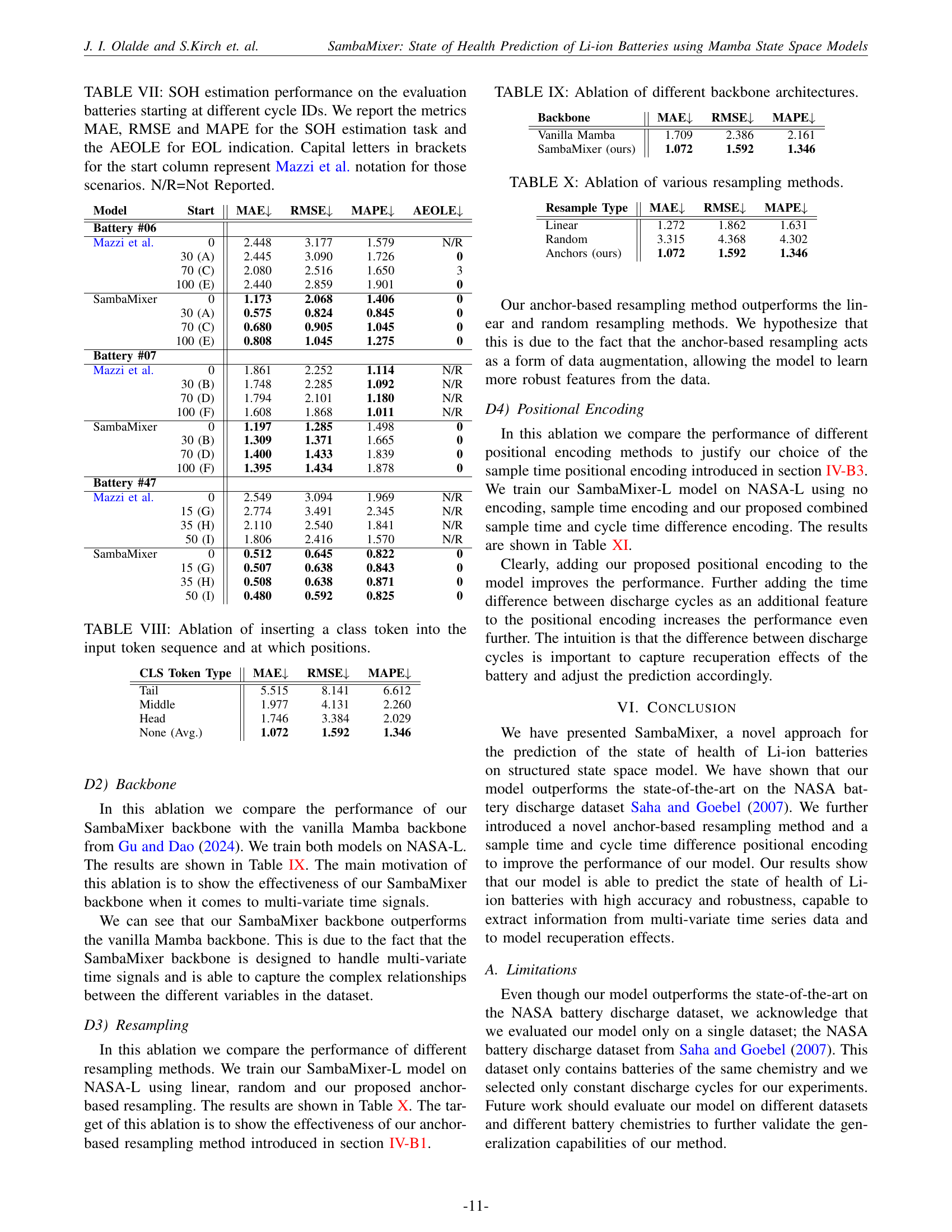
🔼 This figure displays the predicted state of health (SOH) for battery #47 over its lifespan, comparing the model’s prediction to the actual measured SOH. It visualizes the prediction accuracy by showing the difference between the predicted and actual SOH values over a series of discharge cycles. The plot also indicates the predicted end-of-life (EOL) point, comparing it with the actual EOL of the battery. The prediction error is also presented, visually representing the model’s performance in SOH estimation.
read the caption
Figure 7: SOH prediction for Battery #47

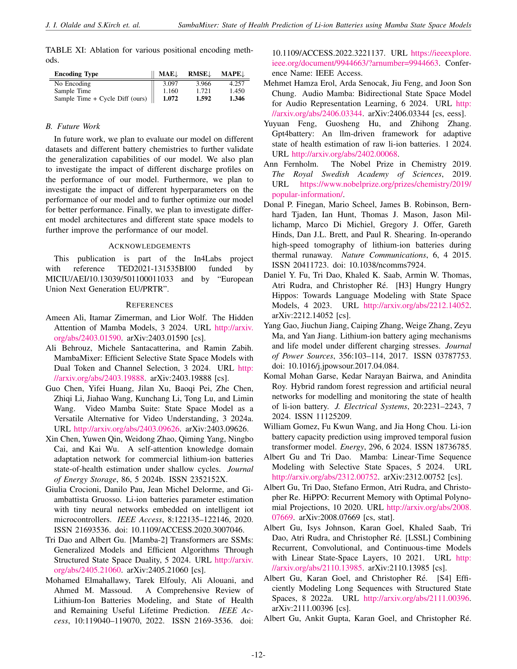
🔼 This figure presents a histogram visualizing the distribution of State of Health (SOH) values from the NASA-L dataset, which is used to train and evaluate a deep learning model for Li-ion battery health prediction. The histogram compares the SOH value distributions for the training and evaluation subsets of the NASA-L dataset, showing how frequently certain SOH ranges appear in each subset. A total of 50 bins were used to create this histogram. The purpose is to illustrate the data’s characteristics and how it might influence the model’s training and evaluation performance. Differences between the training and evaluation distributions might point to potential overfitting or insufficient data representation issues.
read the caption
Figure 8: Histogram of SOH value counts. Comparison of train and eval split of the NASA-L dataset. Number of bins: 50.

🔼 This figure visualizes the results of a model scaling experiment. It shows how the mean absolute error (MAE) in state-of-health (SOH) estimation changes based on different model sizes (S, M, L, XL) and datasets (NASA-S, NASA-M, NASA-L). Each bar represents the MAE achieved by a specific model on a specific dataset. This allows for a direct comparison of performance across different model complexities and data amounts, helping to determine the optimal combination for accurate SOH prediction.
read the caption
Figure 9: Model scaling experiment. MAE metric for the SOH estimation task for different model sizes and datasets. Values are reported in Table VI
More on tables
| ID | Profile | Tamb | VCO | Initial Capacity |
|---|---|---|---|---|
| #5 | (const.) 2.0A | 24 °C | 2.7 V | 1.8565 Ah |
| #6 | (const.) 2.0A | 24 °C | 2.5 V | 2.0353 Ah |
| #7 | (const.) 2.0A | 24 °C | 2.2 V | 1.8911 Ah |
| #18 | (const.) 2.0A | 24 °C | 2.5 V | 1.8550 Ah |
| #25 | (PWM 0.05Hz) 4.0A | 24 °C | 2.0 V | 1.8470 Ah |
| #26 | (PWM 0.05Hz) 4.0A | 24 °C | 2.2 V | 1.8133 Ah |
| #27 | (PWM 0.05Hz) 4.0A | 24 °C | 2.5 V | 1.8233 Ah |
| #28 | (PWM 0.05Hz) 4.0A | 24 °C | 2.7 V | 1.8047 Ah |
| #29 | (const.) 4.0A | 43 °C | 2.0 V | 1.8447 Ah |
| #31 | (const.) 1.5A | 43 °C | 2.5 V | 1.8329 Ah |
| #34 | (const.) 4.0A | 24 °C | 2.2 V | 1.6623 Ah |
| #36 | (const.) 2.0A | 24 °C | 2.7 V | 1.8011 Ah |
| #45 | (const.) 1.0A | 4 °C | 2.0 V | 0.9280 Ah |
| #46 | (const.) 1.0A | 4 °C | 2.2 V | 1.5161 Ah |
| #47 | (const.) 1.0A | 4 °C | 2.5 V | 1.5244 Ah |
| #48 | (const.) 1.0A | 4 °C | 2.7 V | 1.5077 Ah |
| #54 | (const.) 2.0A | 4 °C | 2.2 V | 1.1665 Ah |
| #55 | (const.) 2.0A | 4 °C | 2.5 V | 1.3199 Ah |
| #56 | (const.) 2.0A | 4 °C | 2.7 V | 1.3444 Ah |
🔼 This table details the characteristics of various NASA Lithium-ion batteries used in the experiments. For each battery, it provides the discharge profile (constant current or pulse width modulation), the ambient temperature during the discharge tests, the cut-off voltage at which the discharge cycle ends, and the battery’s initial capacity at the start of the measurement campaign.
read the caption
TABLE II: Discharge specifications for various NASA Li-ion batteries. For the profile we report the discharge current signal form and the discharge amplitude. Tambsubscript𝑇𝑎𝑚𝑏T_{amb}italic_T start_POSTSUBSCRIPT italic_a italic_m italic_b end_POSTSUBSCRIPT is the ambient temperature, VCOsubscript𝑉𝐶𝑂V_{CO}italic_V start_POSTSUBSCRIPT italic_C italic_O end_POSTSUBSCRIPT is the cut-off voltage and Initial Capacity is the initial capacity of the battery at the beginning of the measurement campaign.
| ID | NASA-S | NASA-M | NASA-L |
|---|---|---|---|
| #5 | train | train | train |
| #6 | eval | eval | eval |
| #7 | eval | eval | eval |
| #18 | - | train | train |
| #25 | train | - | - |
| #26 | - | - | - |
| #27 | - | - | - |
| #28 | - | - | - |
| #29 | train | - | - |
| #31 | - | - | train |
| #34 | - | - | train |
| #36 | - | - | train |
| #45 | - | train | train |
| #46 | - | train | train |
| #47 | eval | eval | eval |
| #48 | train | train | train |
| #54 | - | - | train |
| #55 | - | - | train |
| #56 | - | - | train |
🔼 This table details the different training and evaluation splits used for the NASA Li-ion battery datasets in the experiments and ablations of the paper. Each row represents a specific battery ID from the NASA dataset, indicating whether that battery’s data was used for training or evaluation in the various experiments and ablations. The table helps to clarify which datasets were used for model training, validation, and testing purposes, enabling readers to better understand and interpret the results presented in the paper.
read the caption
TABLE III: Different Training and Evaluation splits for the NASA Li-ion batteries used throughout our experiments and ablations.
| Battery | Model | MAE↓ | RMSE↓ | MAPE↓ |
|---|---|---|---|---|
| #06 | Mazzi et al. | 2.448 | 3.177 | 1.579 |
| SambaMixer (ours) | 1.173 | 2.068 | 1.406 | |
| #07 | Mazzi et al. | 1.861 | 2.252 | 1.114 |
| SambaMixer (ours) | 1.197 | 1.285 | 1.498 | |
| #47 | Mazzi et al. | 2.549 | 3.094 | 1.969 |
| SambaMixer (ours) | 0.512 | 0.645 | 0.822 |
🔼 This table compares the performance of the SambaMixer models (introduced in this paper) against the state-of-the-art Mazzi et al. (2024) model for predicting the state-of-health (SOH) of Lithium-ion batteries using the NASA dataset. The comparison uses three common metrics for evaluating regression models: Mean Absolute Error (MAE), Root Mean Squared Error (RMSE), and Mean Absolute Percentage Error (MAPE). The results for each metric are provided for several individual batteries from the NASA dataset, allowing for a battery-by-battery comparison of model accuracy. The best performing model for each battery is indicated in bold.
read the caption
TABLE IV: Comparing our SambaMixer models with the state-of-the-art Mazzi et al. (2024) on the NASA Li-ion batteries. We report the MAE, RMSE and MAPE for each battery. The best results are highlighted in bold.
| Model | Dataset | MAE↓ | RMSE↓ | MAPE↓ |
|---|---|---|---|---|
| Mazzi et al. | NASA-S | 2.220 | 2.778 | 1.451 |
| SambaMixer (ours) | NASA-S | 1.764 | 2.404 | 2.320 |
| NASA-M | 1.334 | 1.902 | 1.641 | |
| NASA-L | 1.072 | 1.592 | 1.346 |
🔼 This table presents a comparison of the SambaMixer model’s performance when trained on different datasets. The model was trained on three variations of the NASA Li-ion battery dataset: NASA-S, NASA-M, and NASA-L, each representing different sizes of data. The evaluation sets remain consistent across all training sets. The table displays the MAE (Mean Absolute Error), RMSE (Root Mean Squared Error), and MAPE (Mean Absolute Percentage Error) metrics for each training set. This allows for a direct comparison of the model’s accuracy and generalization capabilities when trained on datasets with varying data sizes.
read the caption
TABLE V: Performance of our SambaMixer model when trained on different training sets. Evaluation sets are the same for all datasets.
| Model | Dataset | MAE↓ | RMSE↓ | MAPE↓ |
|---|---|---|---|---|
| SambaMixer-S | NASA-S | 2.478 | 3.974 | 3.325 |
| NASA-M | 1.920 | 2.829 | 2.461 | |
| NASA-L | 1.895 | 2.929 | 2.315 | |
| SambaMixer-M | NASA-S | 1.987 | 2.879 | 2.609 |
| NASA-M | 1.736 | 2.414 | 2.170 | |
| NASA-L | 1.230 | 2.027 | 1.493 | |
| SambaMixer-L | NASA-S | 1.764 | 2.404 | 2.320 |
| NASA-M | 1.334 | 1.902 | 1.641 | |
| NASA-L | 1.072 | 1.592 | 1.346 | |
| SambaMixer-XL | NASA-S | 1.693 | 2.431 | 2.218 |
| NASA-M | 1.349 | 1.966 | 1.642 | |
| NASA-L | 1.133 | 1.800 | 1.396 |
🔼 This table presents the results of an experiment assessing the impact of model size and dataset size on the accuracy of State-of-Health (SOH) prediction for lithium-ion batteries. Different sized SambaMixer models (S, M, L, XL) were trained on three datasets (NASA-S, NASA-M, NASA-L) of varying sizes. The table reports the Mean Absolute Error (MAE), Root Mean Squared Error (RMSE), and Mean Absolute Percentage Error (MAPE) for each model-dataset combination, providing a comprehensive view of the model’s scalability and performance across different data conditions.
read the caption
TABLE VI: Model scaling experiment. We report the metrics MAE, RMSE and MAPE for the SOH estimation task for different model sizes and datasets.
| Model | Start | MAE↓ | RMSE↓ | MAPE↓ | AEOLE↓ |
|---|---|---|---|---|---|
| Battery #06 | |||||
| Mazzi et al. | 0 | 2.448 | 3.177 | 1.579 | N/R |
| 30 (A) | 2.445 | 3.090 | 1.726 | 0 | |
| 70 (C) | 2.080 | 2.516 | 1.650 | 3 | |
| 100 (E) | 2.440 | 2.859 | 1.901 | 0 | |
| SambaMixer | 0 | 1.173 | 2.068 | 1.406 | 0 |
| 30 (A) | 0.575 | 0.824 | 0.845 | 0 | |
| 70 (C) | 0.680 | 0.905 | 1.045 | 0 | |
| 100 (E) | 0.808 | 1.045 | 1.275 | 0 | |
| Battery #07 | |||||
| Mazzi et al. | 0 | 1.861 | 2.252 | 1.114 | N/R |
| 30 (B) | 1.748 | 2.285 | 1.092 | N/R | |
| 70 (D) | 1.794 | 2.101 | 1.180 | N/R | |
| 100 (F) | 1.608 | 1.868 | 1.011 | N/R | |
| SambaMixer | 0 | 1.197 | 1.285 | 1.498 | 0 |
| 30 (B) | 1.309 | 1.371 | 1.665 | 0 | |
| 70 (D) | 1.400 | 1.433 | 1.839 | 0 | |
| 100 (F) | 1.395 | 1.434 | 1.878 | 0 | |
| Battery #47 | |||||
| Mazzi et al. | 0 | 2.549 | 3.094 | 1.969 | N/R |
| 15 (G) | 2.774 | 3.491 | 2.345 | N/R | |
| 35 (H) | 2.110 | 2.540 | 1.841 | N/R | |
| 50 (I) | 1.806 | 2.416 | 1.570 | N/R | |
| SambaMixer | 0 | 0.512 | 0.645 | 0.822 | 0 |
| 15 (G) | 0.507 | 0.638 | 0.843 | 0 | |
| 35 (H) | 0.508 | 0.638 | 0.871 | 0 | |
| 50 (I) | 0.480 | 0.592 | 0.825 | 0 |
🔼 Table VII presents a detailed comparison of State-of-Health (SOH) estimation performance across different starting points within the battery discharge cycles for multiple batteries. The evaluation utilizes the same evaluation set across all scenarios. The table compares the performance of the SambaMixer model against results reported by Mazzi et al., offering a comprehensive assessment of predictive accuracy for various stages of battery life. Metrics included are Mean Absolute Error (MAE), Root Mean Square Error (RMSE), Mean Absolute Percentage Error (MAPE), and Absolute End-of-Life Error (AEOLE). The ‘Start’ column indicates the cycle at which the SOH prediction begins, where capital letters within parentheses correspond to scenario labels used by Mazzi et al. ‘N/R’ indicates that Mazzi et al. did not report results for that specific starting point.
read the caption
TABLE VII: SOH estimation performance on the evaluation batteries starting at different cycle IDs. We report the metrics MAE, RMSE and MAPE for the SOH estimation task and the AEOLE for EOL indication. Capital letters in brackets for the start column represent Mazzi et al. notation for those scenarios. N/R=Not Reported.
| CLS Token Type | MAE↓ | RMSE↓ | MAPE↓ |
|---|---|---|---|
| Tail | 5.515 | 8.141 | 6.612 |
| Middle | 1.977 | 4.131 | 2.260 |
| Head | 1.746 | 3.384 | 2.029 |
| None (Avg.) | 1.072 | 1.592 | 1.346 |
🔼 This table presents the results of an ablation study on the impact of using a class token in the SambaMixer model. The study examines different positions for the class token (tail, middle, head) and the effect of omitting it entirely. The table shows the Mean Absolute Error (MAE), Root Mean Square Error (RMSE), and Mean Absolute Percentage Error (MAPE) for each class token configuration and the ’none’ (average) condition. The results help assess the optimal strategy for incorporating class tokens in the model architecture to improve its performance. The results are important for understanding and optimizing the model’s architecture.
read the caption
TABLE VIII: Ablation of inserting a class token into the input token sequence and at which positions.
| Backbone | MAE ↓ | RMSE ↓ | MAPE ↓ |
|---|---|---|---|
| Vanilla Mamba | 1.709 | 2.386 | 2.161 |
| SambaMixer (ours) | 1.072 | 1.592 | 1.346 |
🔼 This table presents an ablation study comparing the performance of two different backbone architectures: a vanilla Mamba model and the SambaMixer model proposed in the paper. The comparison is done using the MAE, RMSE, and MAPE metrics, providing a quantitative assessment of the impact of the SambaMixer architecture on the model’s accuracy in predicting the state of health of lithium-ion batteries.
read the caption
TABLE IX: Ablation of different backbone architectures.
| Resample Type | MAE↓ | RMSE↓ | MAPE↓ |
|---|---|---|---|
| Linear | 1.272 | 1.862 | 1.631 |
| Random | 3.315 | 4.368 | 4.302 |
| Anchors (ours) | 1.072 | 1.592 | 1.346 |
🔼 This table presents the results of an ablation study comparing different resampling methods used in the SambaMixer model for predicting the State of Health (SOH) of Li-ion batteries. The methods compared are linear resampling, random resampling, and the proposed anchor-based resampling. The table shows the Mean Absolute Error (MAE), Root Mean Square Error (RMSE), and Mean Absolute Percentage Error (MAPE) for each resampling technique, allowing for a quantitative comparison of their effectiveness. The results highlight the relative performance of different methods for handling variations in sample lengths across different discharge cycles of batteries.
read the caption
TABLE X: Ablation of various resampling methods.
| Encoding Type | MAE↓ | RMSE↓ | MAPE↓ |
|---|---|---|---|
| No Encoding | 3.097 | 3.966 | 4.257 |
| Sample Time | 1.160 | 1.721 | 1.450 |
| Sample Time + Cycle Diff (ours) | 1.072 | 1.592 | 1.346 |
🔼 This table presents an ablation study on the impact of different positional encoding methods on the performance of the SambaMixer model for predicting the state-of-health of Li-ion batteries. The study compares three methods: no positional encoding, sample time positional encoding, and combined sample time and cycle time difference positional encoding. The results show the MAE, RMSE, and MAPE for each method, demonstrating the effectiveness of incorporating both sample time and cycle time difference for improved prediction accuracy.
read the caption
TABLE XI: Ablation for various positional encoding methods.
Full paper#
