TL;DR#
Diffusion models generate high-quality images but are computationally expensive due to their multi-step generation process. Prior methods like Rectified Flow attempted to speed this up by straightening ODE flow trajectories, but limitations remained, particularly in accurately learning straight trajectories and achieving optimal few-step generation. These limitations stemmed from approximating couplings (image and noise pairs) with constant velocity, which often resulted in suboptimal performance and curved sampling trajectories.
To address this, the authors introduce Constant Acceleration Flow (CAF), which models couplings using a simple constant acceleration equation instead of constant velocity. CAF introduces acceleration as an additional learnable variable, enabling more accurate and expressive ODE flow estimation. Moreover, to further improve accuracy, they propose two techniques: initial velocity conditioning for the acceleration model and a reflow process for the initial velocity. Extensive experiments on various datasets demonstrate that CAF significantly outperforms state-of-the-art baselines, exhibiting superior performance in both one-step and few-step generation while preserving coupling and inversion more effectively.
Key Takeaways#
Why does it matter?#
This paper is important because it significantly advances fast generation in diffusion models, a crucial area of current research. The introduction of Constant Acceleration Flow (CAF) offers a novel approach that outperforms existing methods in terms of speed and accuracy, paving the way for more efficient and high-quality generative models. The paper also proposes techniques to address limitations in existing methods, leading to improved performance in few-step generation and enhanced coupling preservation. This work opens avenues for further exploration in developing more sophisticated ODE-based generative models and improving their efficiency for various real-world applications.
Visual Insights#

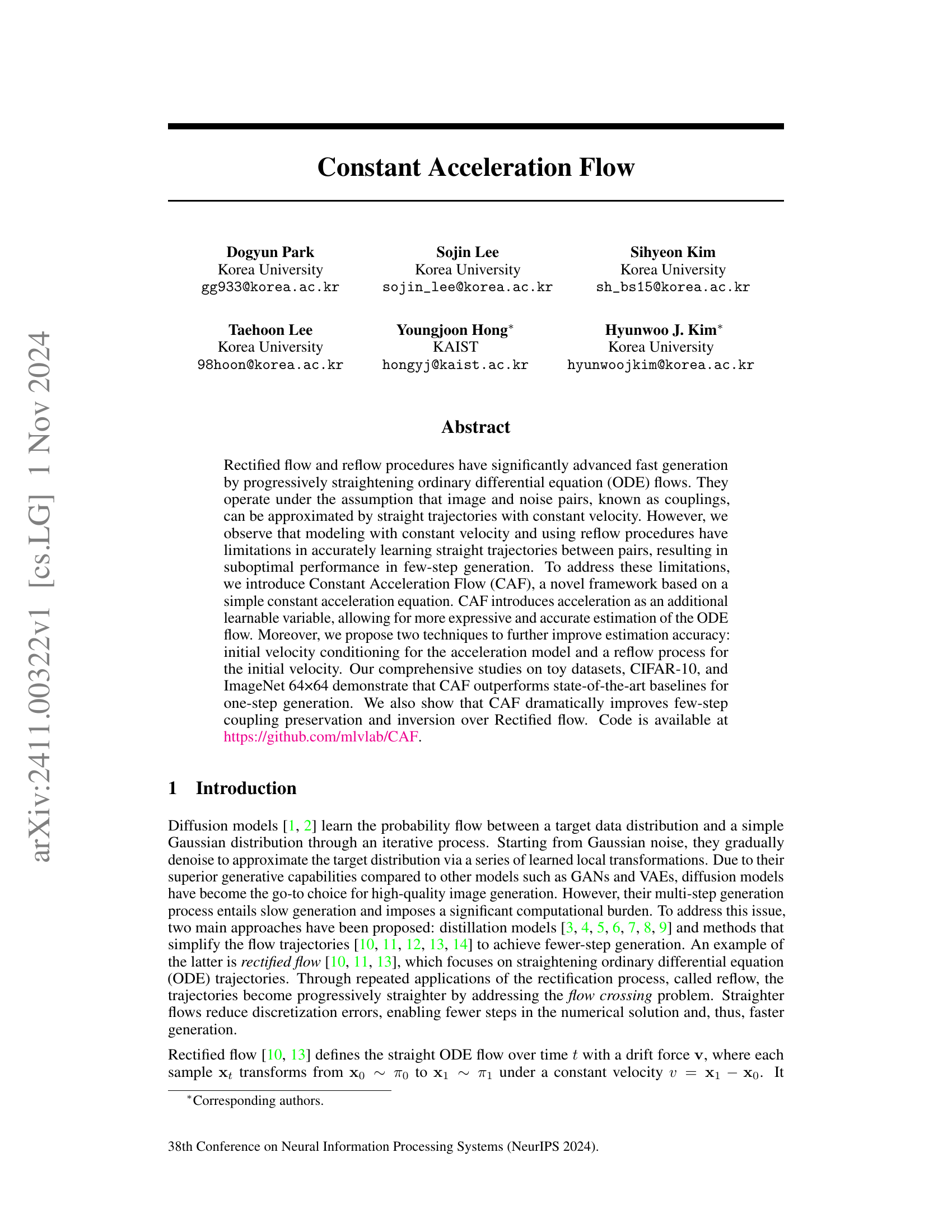
🔼 This figure compares the sampling trajectories of Rectified Flow and Constant Acceleration Flow (CAF). Rectified Flow, shown in (a), uses a constant velocity model for estimating the ODE flow. Due to limitations of this model in accurately capturing the relationship between image-noise pairs, it produces curved trajectories and flow crossing, as seen at the intersection point (x = x^2). In contrast, CAF, shown in (b), incorporates a constant acceleration term as an additional learnable variable, resulting in improved flow estimation accuracy and straighter trajectories that accurately reflect the ground truth trajectory, minimizing flow crossing and improving the precision of ODE flow estimation.
read the caption
(a) Rectified Flow
In-depth insights#
Accel Flow Intro#
The Accel Flow Intro section introduces Constant Acceleration Flow (CAF), a novel framework that addresses limitations of existing rectified flow models in accurately learning straight trajectories for image generation. CAF incorporates acceleration as a learnable variable, moving beyond the constant velocity assumption of previous methods. This enhancement allows for more expressive and accurate estimation of the ODE flow, significantly improving performance. The introduction also highlights the issue of flow crossing, where sampling trajectories intersect, leading to suboptimal results, and previews CAF’s innovative solutions to this problem, including initial velocity conditioning (IVC) and a reflow process to improve accuracy and avoid curved trajectories. The section concludes by emphasizing CAF’s superior performance over current state-of-the-art methods for one-step and few-step image generation.
IVC & Reflow#
To overcome the limitations of constant velocity modeling in rectified flow, which struggles with accurately learning straight trajectories due to flow crossing, the authors introduce initial velocity conditioning (IVC) and reflow procedures within their Constant Acceleration Flow (CAF) framework. IVC conditions the acceleration model on the estimated initial velocity, thereby reducing ambiguity and improving trajectory estimation, especially near intersection points. The reflow process further enhances accuracy by refining the initial velocity learning using a pre-trained generative model to create more deterministic data couplings. These two strategies work synergistically to address flow crossing, resulting in more accurate and efficient learning of straight ODE trajectories, as demonstrated in the superior performance of CAF over baseline methods in one-step and few-step generation tasks.
Synthetic & Real Data#
The paper evaluates Constant Acceleration Flow (CAF) using synthetic and real-world datasets. Synthetic experiments on a 2D dataset demonstrate CAF’s superior accuracy in approximating target distributions compared to Rectified Flow, especially when using negative acceleration. Real-world experiments on CIFAR-10 and ImageNet 64x64 show CAF achieving state-of-the-art FID scores, highlighting its ability to generate high-quality images even with one-step generation. In both cases, the introduction of acceleration as a learnable parameter and the initial velocity conditioning proved crucial for improved performance, substantially reducing the impact of flow crossings. The ablation study further confirms these findings, emphasizing the importance of each component of the CAF framework.
Coupling Analysis#
The Coupling Analysis section delves into the accuracy of approximating deterministic couplings in both CAF and Rectified Flow. Synthetic experiments reveal CAF’s superior ability to preserve ground-truth couplings, particularly when flow crossing occurs. This is demonstrated through visual comparisons of sampling trajectories, showing that CAF maintains straight trajectories while Rectified Flow produces curved ones. Real-world CIFAR-10 experiments using LPIPS and PSNR metrics further solidify CAF’s advantage. CAF exhibits significantly lower LPIPS scores and higher PSNR values, signifying better preservation of the original data relationships. The superior performance of CAF in preserving couplings underscores its enhanced expressiveness in modeling complex relationships between data points, leading to more accurate and reliable generative results. This improved coupling preservation is crucial for achieving high-quality image generation, especially when dealing with few sampling steps.
Limitations & Future#
The authors acknowledge that their Constant Acceleration Flow (CAF) model, while improving speed and quality in image generation, has limitations. Increased computational cost compared to Rectified Flow is a primary concern due to the additional calculation of acceleration at each step. Improving efficiency through techniques like jointly predicting velocity and acceleration is suggested for future work. Additionally, the need for supplementary data generation for optimal model training adds to resource consumption. Future research should focus on addressing these limitations to make CAF more efficient and resource-friendly, potentially exploring alternative training strategies or model architectures that minimize computational overhead while retaining performance advantages.
More visual insights#
More on figures

🔼 This figure, part (b) of Figure 1, illustrates the Constant Acceleration Flow (CAF) and how it addresses the flow crossing problem inherent in ODE flow models. In contrast to Rectified Flow (part (a)), CAF introduces acceleration as a learnable parameter, enabling a more accurate representation of the ODE trajectories between the source and target data distributions. Specifically, the diagram shows that CAF, utilizing Initial Velocity Conditioning (IVC), successfully minimizes ambiguity at the point where flow crossing occurs (x=x²), resulting in accurate and smoother sampling trajectories.
read the caption
(b) Constant Acceleration Flow

🔼 This figure compares the performance of Rectified Flow and Constant Acceleration Flow (CAF) in addressing the flow crossing problem. Rectified Flow, shown in (a), attempts to model the flow between data points using constant velocity, resulting in approximation errors and curved sampling trajectories when trajectories intersect at a point xt where xt1 = xt2. In contrast, CAF, shown in (b), uses Initial Velocity Conditioning (IVC) to incorporate acceleration as a learnable variable. This allows CAF to more accurately estimate ground-truth trajectories by mitigating the ambiguity at intersection points and minimizing curved paths.
read the caption
Figure 1: Initial Velocity Conditioning (IVC). We illustrate the importance of IVC to address the flow crossing problem, which hinders the learning of straight ODE trajectories during training. In Fig. 1(a), Rectified flow suffers from approximation errors at the overlapping point 𝐱tsubscript𝐱𝑡\mathbf{x}_{t}bold_x start_POSTSUBSCRIPT italic_t end_POSTSUBSCRIPT (where 𝐱t1=𝐱t2superscriptsubscript𝐱𝑡1superscriptsubscript𝐱𝑡2\mathbf{x}_{t}^{1}=\mathbf{x}_{t}^{2}bold_x start_POSTSUBSCRIPT italic_t end_POSTSUBSCRIPT start_POSTSUPERSCRIPT 1 end_POSTSUPERSCRIPT = bold_x start_POSTSUBSCRIPT italic_t end_POSTSUBSCRIPT start_POSTSUPERSCRIPT 2 end_POSTSUPERSCRIPT), resulting in curved sampling trajectories due to flow crossing. Conversely, Fig. 1(b) demonstrates that CAF, utilizing IVC, successfully estimates ground-truth trajectories by minimizing the ambiguity at 𝐱tsubscript𝐱𝑡\mathbf{x}_{t}bold_x start_POSTSUBSCRIPT italic_t end_POSTSUBSCRIPT.

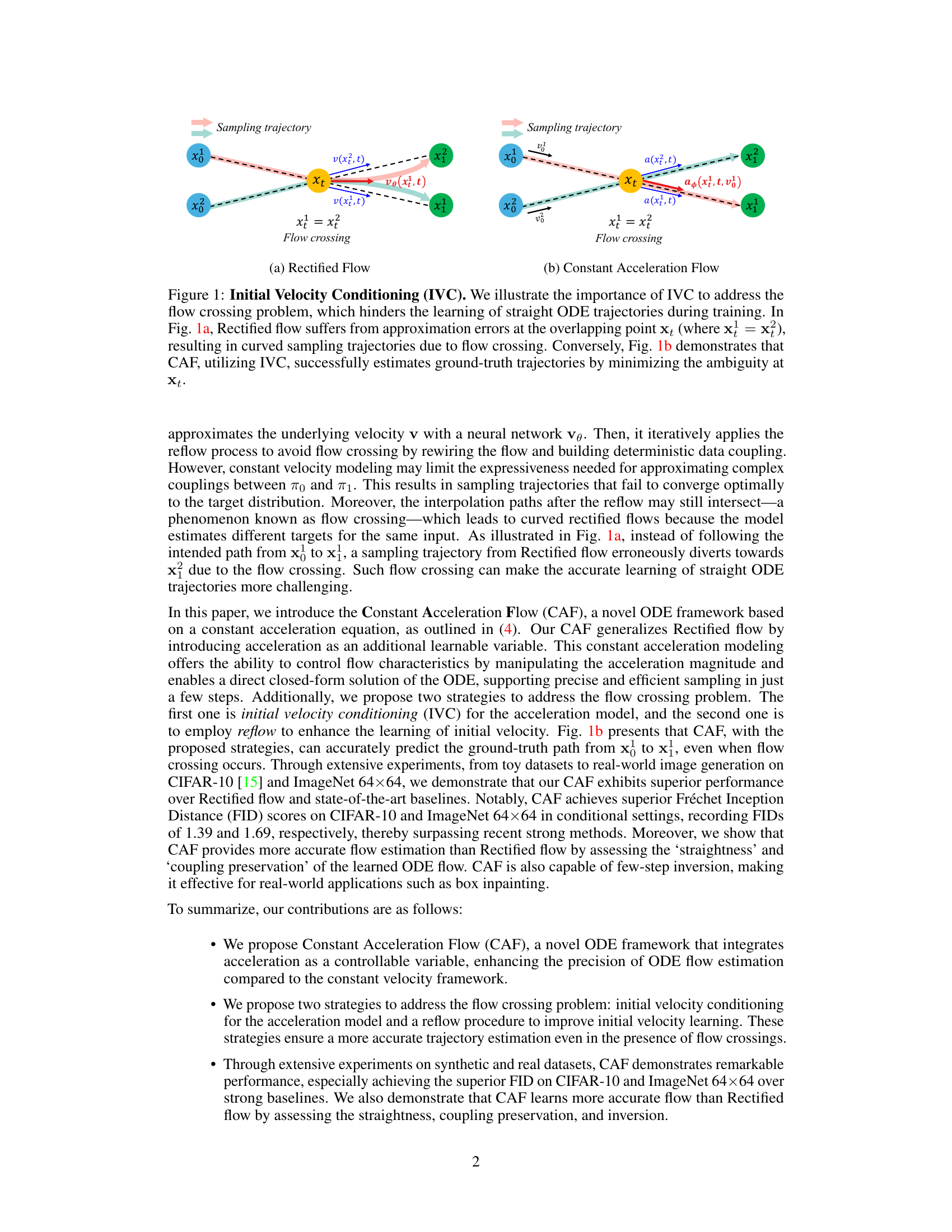
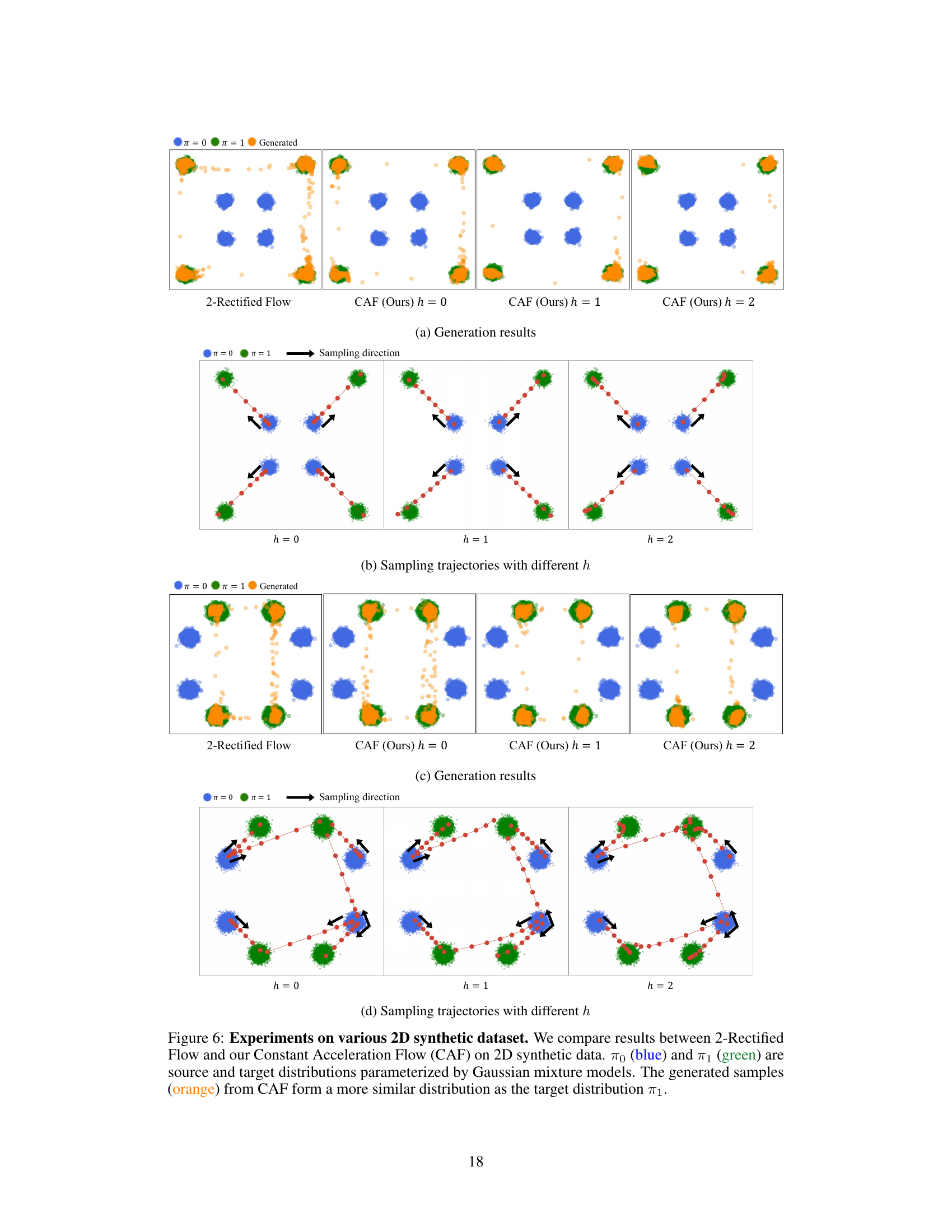
🔼 Figure 2 displays a comparison of sample generation results between the 2-Rectified Flow and the Constant Acceleration Flow (CAF) methods using a 2D synthetic dataset. The source distribution (π₀, blue) and target distribution (π₁, green) are modeled using Gaussian mixture models. The experiment uses a single sampling step (N=1). The figure shows that 2-Rectified Flow often produces samples that deviate significantly from the target distribution (π₁). In contrast, CAF generates samples (orange) that closely match the target distribution (π₁), demonstrating its superior accuracy in estimating the target distribution.
read the caption
Figure 2: 2D synthetic dataset. We compare results between 2-Rectified flow and our Constant Acceleration Flow (CAF) on 2D synthetic data. π0subscript𝜋0\pi_{0}italic_π start_POSTSUBSCRIPT 0 end_POSTSUBSCRIPT (blue) and π1subscript𝜋1\pi_{1}italic_π start_POSTSUBSCRIPT 1 end_POSTSUBSCRIPT (green) are source and target distributions parameterized by Gaussian mixture models. Here, the number of sampling steps is N=1𝑁1N=1italic_N = 1. While 2-Rectified flow frequently generates samples that deviate from π1subscript𝜋1\pi_{1}italic_π start_POSTSUBSCRIPT 1 end_POSTSUBSCRIPT, CAF more accurately estimates the target distribution π1subscript𝜋1\pi_{1}italic_π start_POSTSUBSCRIPT 1 end_POSTSUBSCRIPT. The generated samples (orange) from CAF form a more similar distribution as the target distribution π1subscript𝜋1\pi_{1}italic_π start_POSTSUBSCRIPT 1 end_POSTSUBSCRIPT.

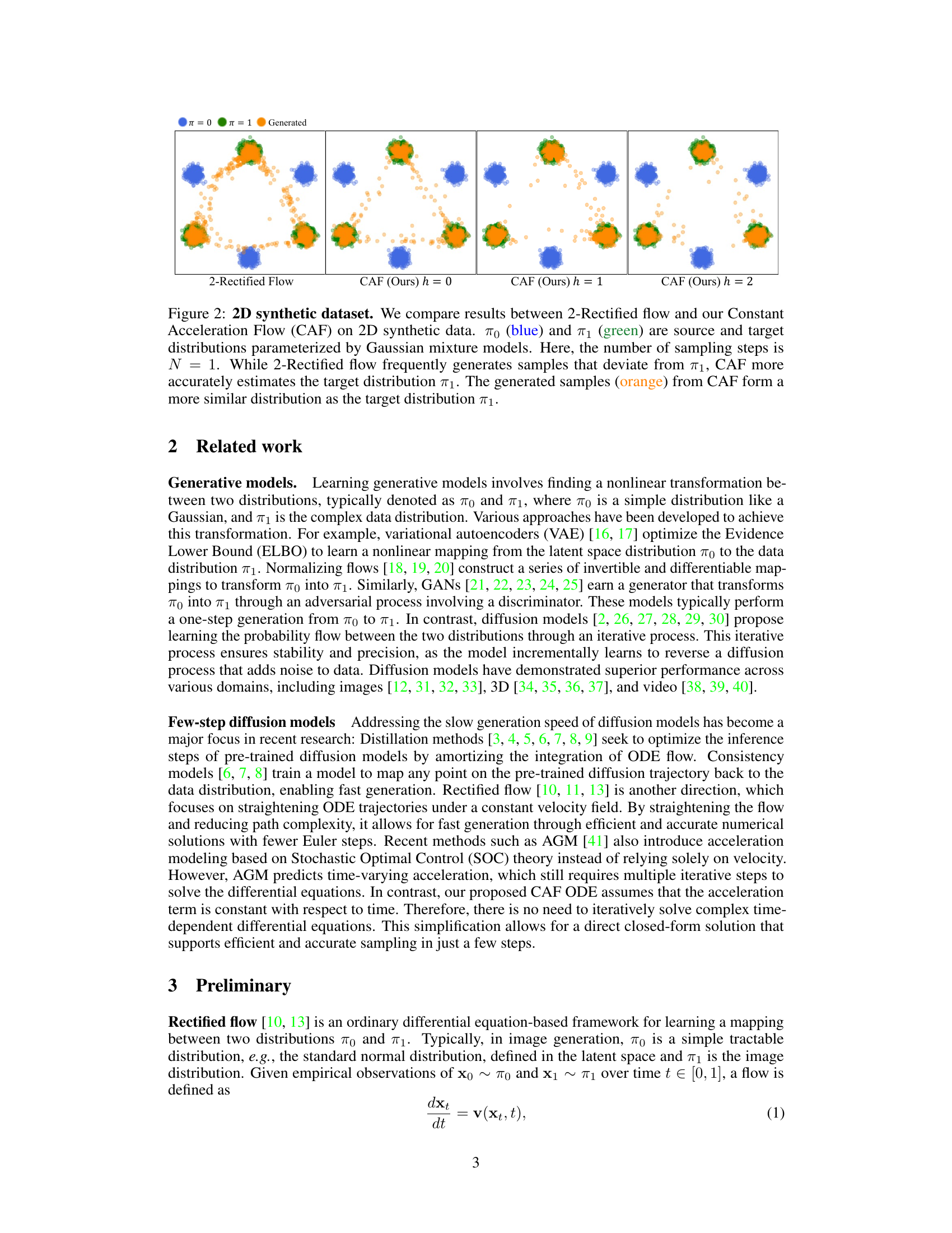
🔼 This figure visualizes how different initial velocities, controlled by the hyperparameter h, influence the sampling trajectories in the Constant Acceleration Flow (CAF) model. The plots show trajectories generated by sampling across seven steps (N=7) starting from a mixture of Gaussian distributions (π0) and aiming for another mixture of Gaussians (π1). The variations in trajectories for different values of h demonstrate CAF’s ability to adjust its flow characteristics through the initial velocity, resulting in different paths to reach the target distribution. This highlights CAF’s flexibility in modeling complex couplings between initial and target distributions.
read the caption
Figure 3: Sampling trajectories of CAF with different hℎhitalic_h. The sampling trajectories of CAF are displayed for different values of hℎhitalic_h, which determines the initial velocity and acceleration. π0subscript𝜋0\pi_{0}italic_π start_POSTSUBSCRIPT 0 end_POSTSUBSCRIPT and π1subscript𝜋1\pi_{1}italic_π start_POSTSUBSCRIPT 1 end_POSTSUBSCRIPT are mixtures of Gaussian distributions. We sample across sampling steps of N=7𝑁7N=7italic_N = 7 to show how sampling trajectories change with hℎhitalic_h.

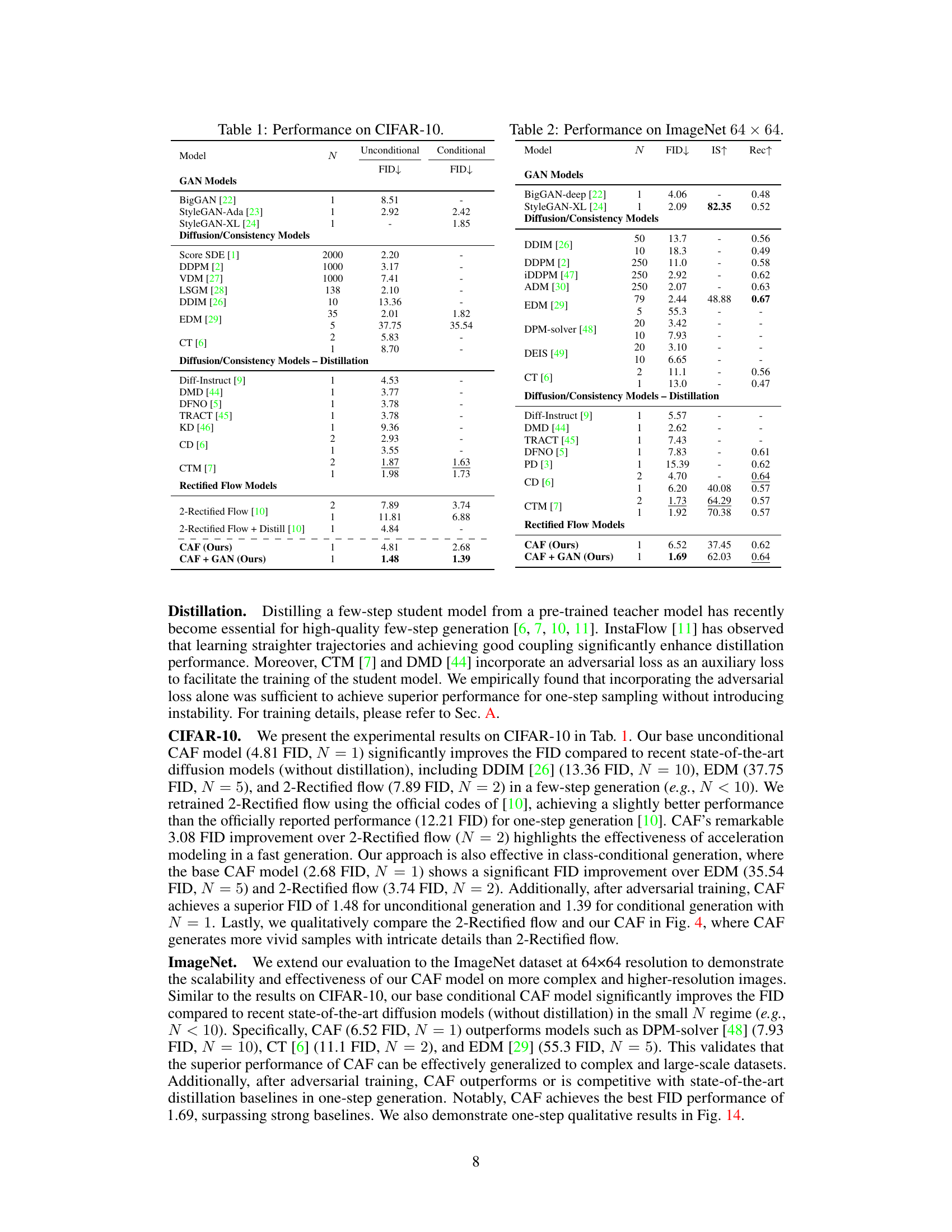
🔼 This table presents a comparison of the performance of various generative models on the ImageNet 64x64 dataset. The models are evaluated based on their Fréchet Inception Distance (FID) scores, which measure the quality of generated images by comparing their distribution to the true ImageNet distribution. Lower FID scores indicate better performance. Additionally, Inception Scores (IS) and recall are provided to give a more comprehensive evaluation of the models’ ability to generate high-quality and diverse images. The table breaks down the performance of different model types, including GANs, diffusion models, consistency models, and the proposed Constant Acceleration Flow (CAF) model. Different numbers of sampling steps (N) are also considered to assess the trade-off between speed and image quality.
read the caption
Table 2: Performance on ImageNet 64×64646464\times 6464 × 64.

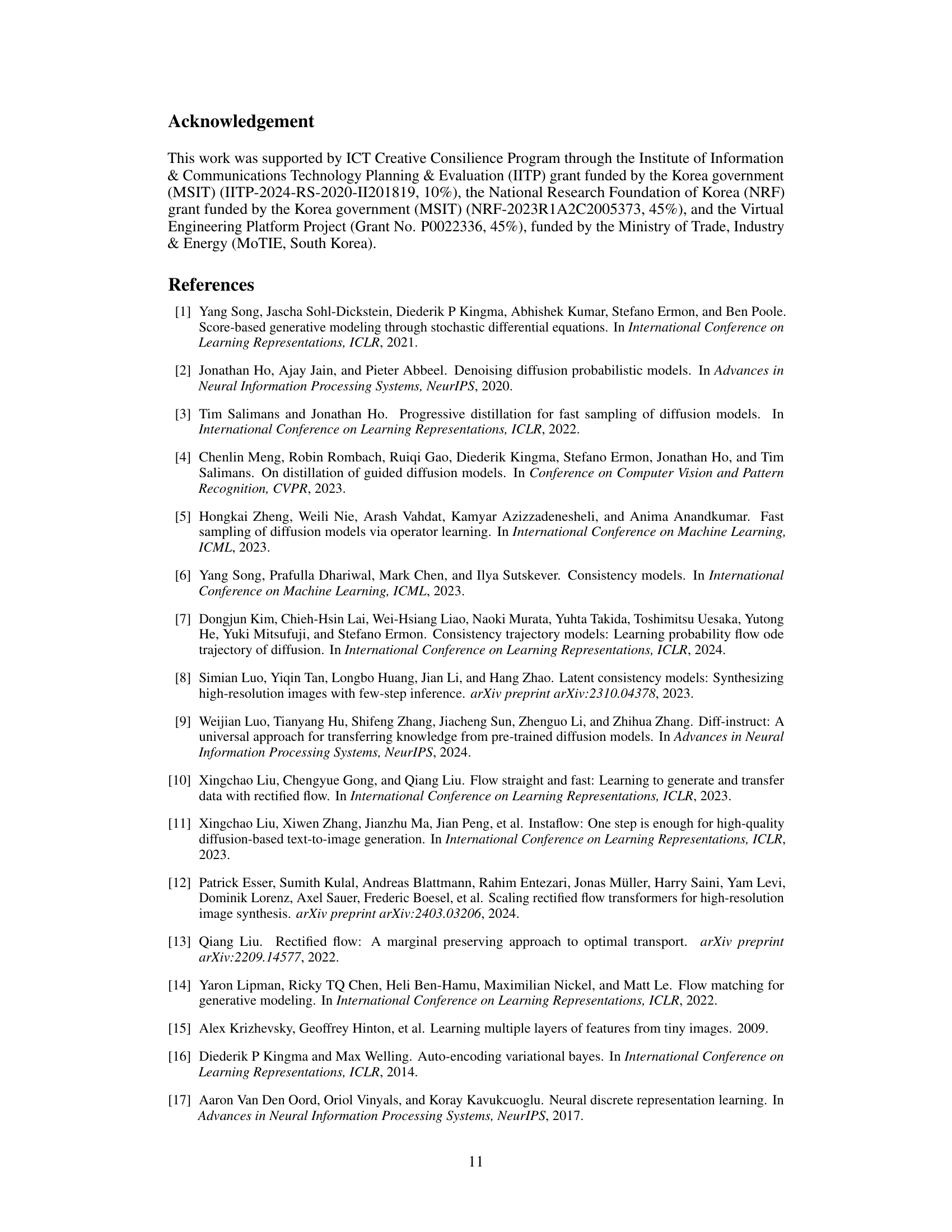
🔼 This figure compares the sampling trajectories of Rectified Flow and Constant Acceleration Flow (CAF) during training. Rectified flow, due to flow crossing issues, results in curved trajectories that deviate from the intended path between data points (x0 and x1). In contrast, CAF, utilizing Initial Velocity Conditioning (IVC), effectively learns straight trajectories by mitigating the ambiguity at the intersection points, leading to more accurate estimation of ODE flows.
read the caption
(a)

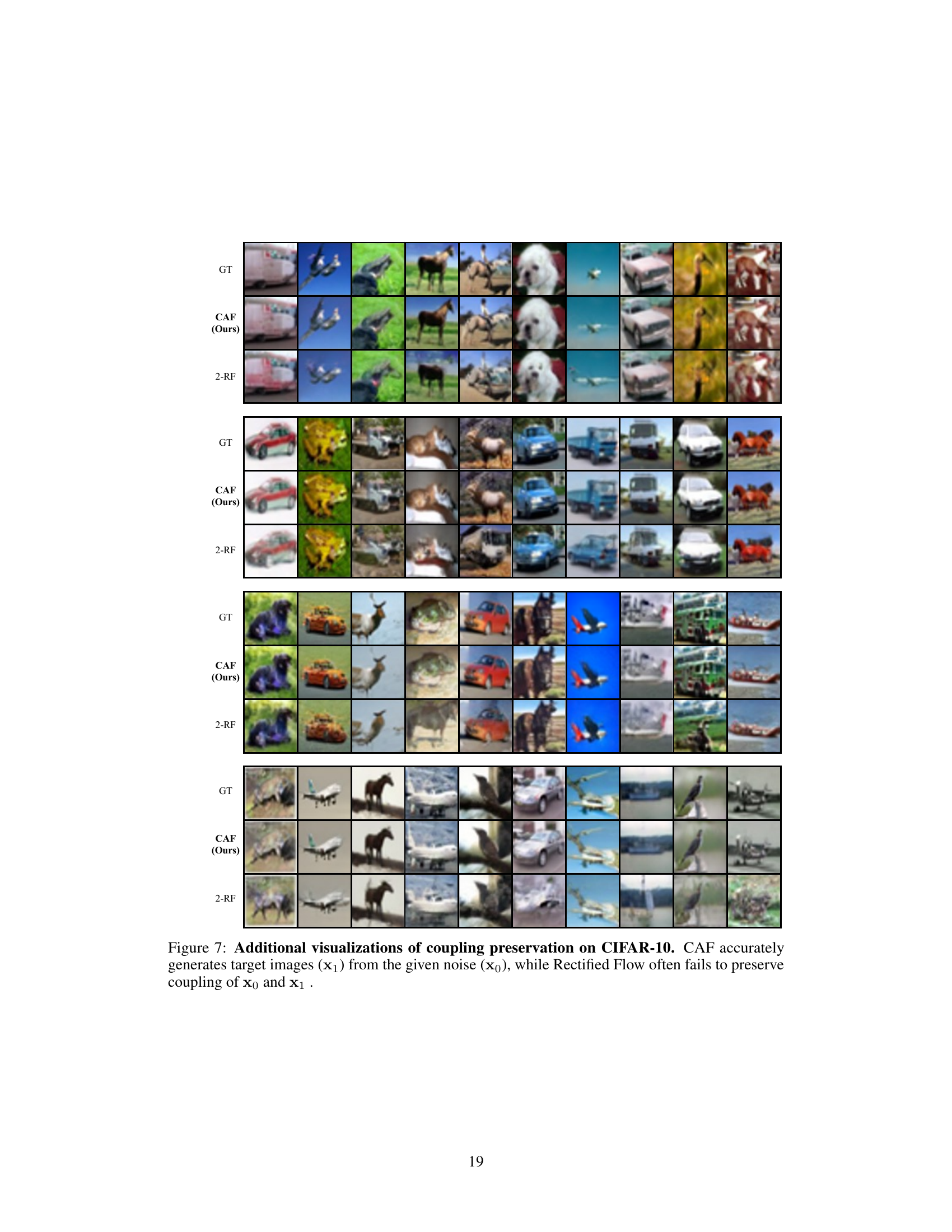
🔼 This figure shows a comparison of coupling preservation between Rectified Flow and CAF. The top row shows the ground truth (GT) coupling. The second row displays the results from 2-Rectified Flow (2-RF). The bottom row shows the results obtained using CAF. Each column represents a different image pair, demonstrating how CAF preserves the coupling more accurately than Rectified Flow, especially when the sampling trajectories would otherwise intersect (flow crossing). The LPIPS scores are shown in parentheses to quantitatively assess the similarity of the generated image to the ground truth.
read the caption
(b)

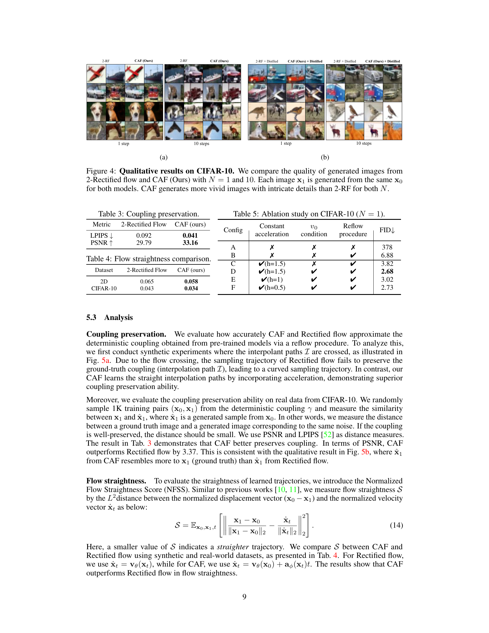
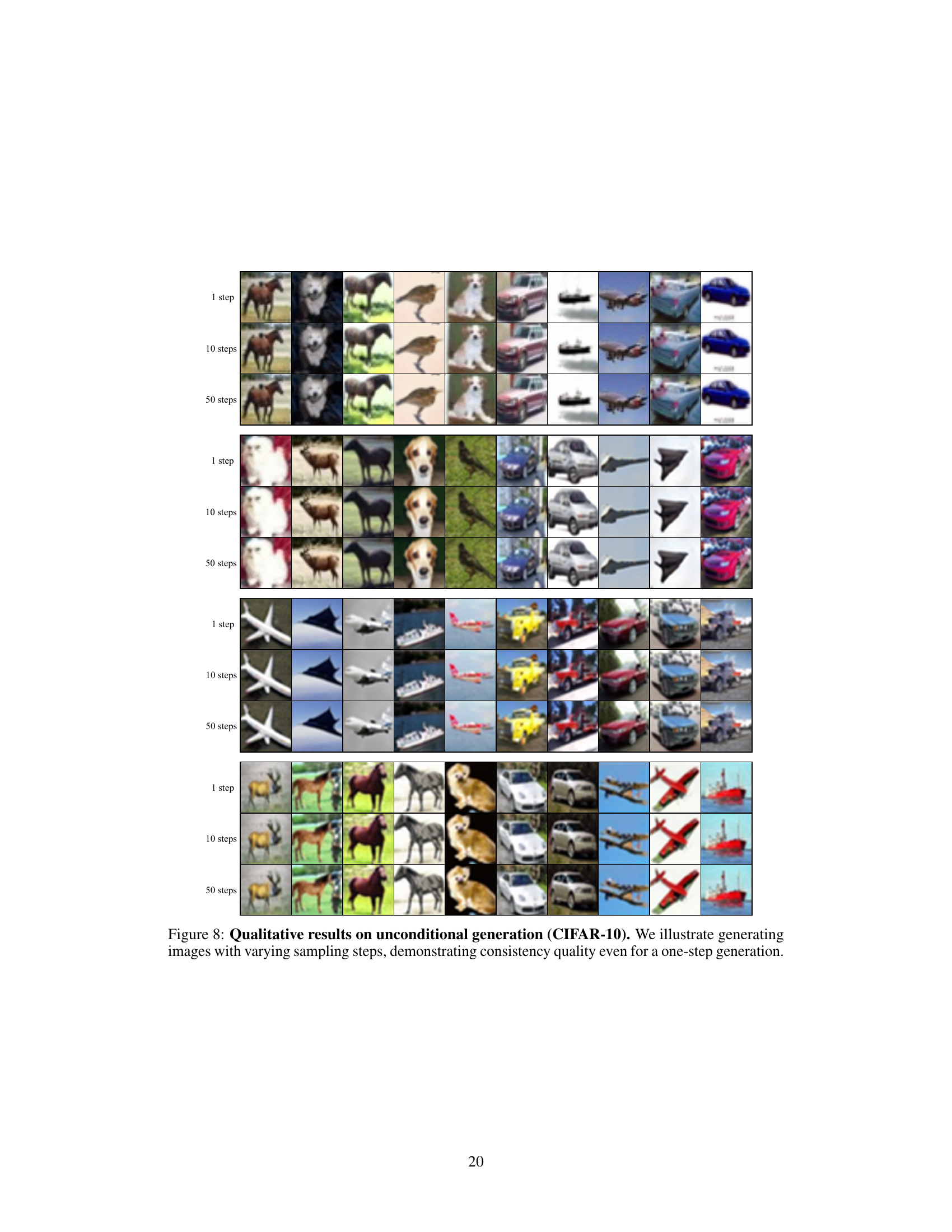
🔼 Figure 4 presents a qualitative comparison of image generation results between the 2-Rectified Flow model and the Constant Acceleration Flow (CAF) model proposed in the paper. The comparison is done using the CIFAR-10 dataset, a standard benchmark for image generation. Two different numbers of sampling steps (N=1 and N=10) are used to generate images. For each setting, the same input noise vector, 𝐱0, is fed to both models. The resulting generated images, 𝐱1, are then displayed. The figure demonstrates that CAF generates images that are visually more realistic and detailed than 2-Rectified Flow, particularly when using fewer sampling steps (N=1). This improved quality highlights the advantages of CAF in generating high-quality images efficiently.
read the caption
Figure 4: Qualitative results on CIFAR-10. We compare the quality of generated images from 2-Rectified flow and CAF (Ours) with N=1𝑁1N=1italic_N = 1 and 10101010. Each image 𝐱1subscript𝐱1\mathbf{x}_{1}bold_x start_POSTSUBSCRIPT 1 end_POSTSUBSCRIPT is generated from the same 𝐱0subscript𝐱0\mathbf{x}_{0}bold_x start_POSTSUBSCRIPT 0 end_POSTSUBSCRIPT for both models. CAF generates more vivid images with intricate details than 2-RF for both N𝑁Nitalic_N.

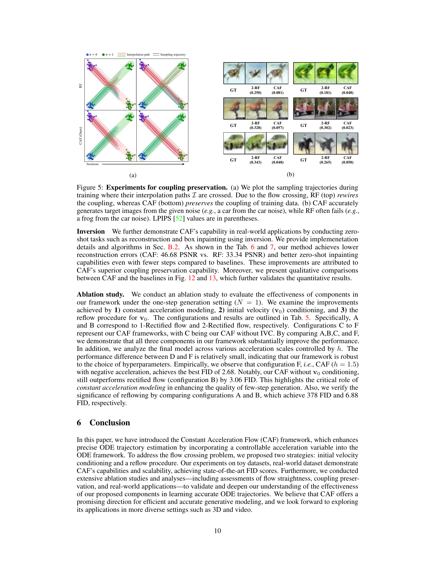
🔼 This table presents a quantitative comparison of coupling preservation between the 2-Rectified Flow and the proposed Constant Acceleration Flow (CAF). Coupling preservation refers to how well the model maintains the relationships between the initial noise (x0) and the target image (x1) during the generation process. The table shows the LPIPS (Learned Perceptual Image Patch Similarity) score and the PSNR (Peak Signal-to-Noise Ratio) between the generated image from the initial noise and the ground truth image from the training data. Lower LPIPS scores indicate better perceptual similarity, while higher PSNR values indicate better structural similarity.
read the caption
Table 3: Coupling preservation.

🔼 This table compares the straightness of the learned ODE trajectories for two different models, 2-Rectified Flow and CAF (Constant Acceleration Flow), across two datasets: a synthetic 2D dataset and the CIFAR-10 dataset. The straightness is measured using the Normalized Flow Straightness Score (NFSS), which quantifies how closely the learned trajectory follows a straight line. Lower scores indicate greater straightness and better efficiency. The results show that CAF achieves a lower NFSS score than 2-Rectified Flow, indicating that CAF learns straighter ODE trajectories.
read the caption
Table 4: Flow straightness comparison.

🔼 This table presents the results of an ablation study conducted on the CIFAR-10 dataset using a one-step generation model (N=1). The study systematically examines the contribution of different components within the Constant Acceleration Flow (CAF) framework. Specifically, it compares the performance of various configurations, including baselines (Rectified Flow and 2-Rectified Flow), and versions of CAF with or without initial velocity conditioning (IVC) and/or a reflow procedure. The primary metric used for evaluation is the Fréchet Inception Distance (FID), a measure of image quality. This allows for a quantitative assessment of the impact of each individual component on the overall model performance.
read the caption
Table 5: Ablation study on CIFAR-10 (N=1𝑁1N=1italic_N = 1).

🔼 This figure shows a comparison of sampling trajectories between Rectified Flow and CAF on a 2D synthetic dataset. The blue and green dots represent the source (π₀) and target (π₁) distributions respectively, while the orange dots show the generated samples. Rectified flow frequently produces samples that deviate from the target distribution, while CAF’s samples are much closer to the target. Different subplots illustrate this comparison for different values of h, a hyperparameter controlling the initial velocity in CAF, demonstrating how CAF’s sampling trajectories change.
read the caption
(a)

🔼 This figure shows qualitative results comparing the performance of 2-Rectified Flow and CAF on CIFAR-10. For both models, images are generated from the same starting noise (x0) for both one step (N=1) and ten steps (N=10). The comparison highlights the superior image quality produced by CAF, which generates more vivid images with finer details than 2-Rectified Flow in both cases.
read the caption
(b)

🔼 Figure 5 demonstrates how Constant Acceleration Flow (CAF) addresses the flow crossing problem, which hinders the accurate learning of straight ODE trajectories during training. Panel (a) shows sampling trajectories for both Rectified Flow (RF) and CAF. RF’s trajectories intersect due to the flow crossing problem, which results in the model learning inaccurate trajectories and rewiring the flow. CAF, however, successfully preserves the coupling between the source (x0) and target (x1) distributions by accurately learning straight trajectories without intersections. Panel (b) illustrates the improved image generation results of CAF compared to RF. CAF accurately generates target images from a given noise, for example, a car from car noise, while RF often fails, generating unrelated images (e.g., a frog from car noise). LPIPS (Learned Perceptual Image Patch Similarity) scores quantify the perceptual difference between the ground truth images and the generated images.
read the caption
Figure 5: Experiments for coupling preservation. (a) We plot the sampling trajectories during training where their interpolation paths ℐℐ\mathcal{I}caligraphic_I are crossed. Due to the flow crossing, RF (top) rewires the coupling, whereas CAF (bottom) preserves the coupling of training data. (b) CAF accurately generates target images from the given noise (e.g., a car from the car noise), while RF often fails (e.g., a frog from the car noise). LPIPS [52] values are in parentheses.

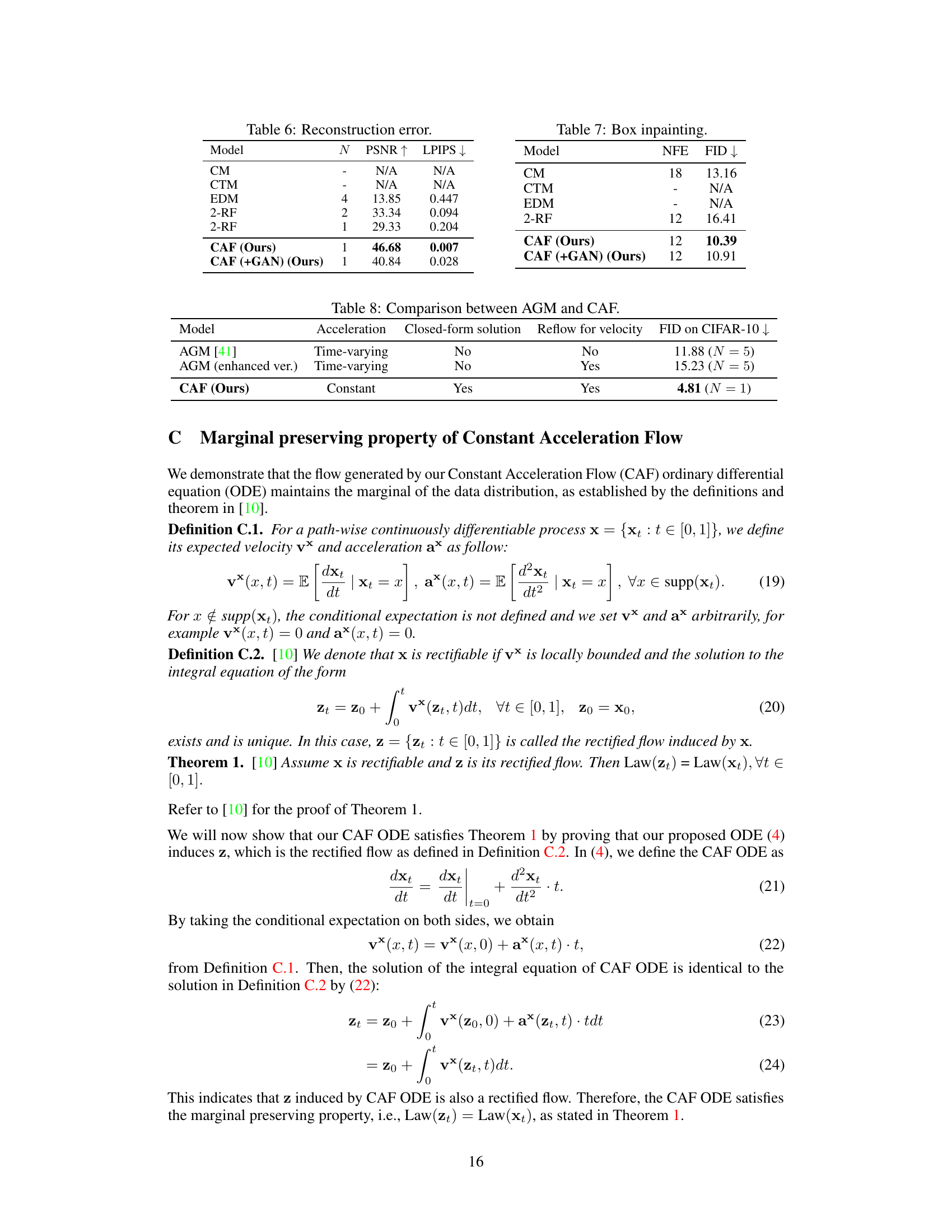
🔼 This table presents a quantitative comparison of reconstruction error achieved by different models. The models are evaluated on their ability to reconstruct an image from its encoded representation. Lower values of PSNR (Peak Signal-to-Noise Ratio) and LPIPS (Learned Perceptual Image Patch Similarity) indicate better reconstruction quality, meaning a more accurate reproduction of the original image.
read the caption
Table 6: Reconstruction error.

🔼 This table presents the results of a box inpainting task, a real-world application of the proposed Constant Acceleration Flow (CAF) model. It compares the performance of CAF against several baseline models (CM, CTM, 2-Rectified Flow) in terms of FID (Fréchet Inception Distance) scores. The number of forward diffusion steps (NFE) used by each model is also shown. Lower FID scores indicate better image quality, reflecting how well the model reconstructs the missing parts of the image. The table demonstrates the superior performance of CAF in this task, achieving lower FID scores with fewer steps than the baselines. This highlights CAF’s efficiency and accuracy in a practical application.
read the caption
Table 7: Box inpainting.

🔼 This table compares the performance of Constant Acceleration Flow (CAF) and Accelerated Gradient Method (AGM). It highlights key differences in their approach to modeling acceleration (constant vs. time-varying), the presence of a closed-form solution for sampling, whether a reflow process is employed for improving velocity estimation, and the resulting FID scores achieved on the CIFAR-10 dataset. The table showcases CAF’s advantage in terms of computational efficiency and performance, as it achieves significantly better FID scores with a simpler, constant acceleration model and one-step sampling.
read the caption
Table 8: Comparison between AGM and CAF.

🔼 This figure shows the results of generating samples from different models on 2D synthetic datasets. The top row displays the results from a 2-Rectified Flow model, while the subsequent rows show results from a Constant Acceleration Flow (CAF) model with different hyperparameters (h = 0, 1, 2). Each model’s output is visualized with colored points, with the starting distribution represented in blue and the target distribution in green. The generated samples are shown in orange. The image helps visualize the effectiveness of CAF in accurately generating samples that closely resemble the target distribution compared to 2-Rectified Flow. The different values of ‘h’ highlight how the initial velocity influences the generated samples, showcasing the model’s flexibility.
read the caption
(a) Generation results

🔼 This figure visualizes how different values of the hyperparameter h influence the sampling trajectories in the Constant Acceleration Flow (CAF) model. The hyperparameter h scales the initial velocity, which in turn affects the acceleration and overall trajectory shape. The figure shows trajectories for three distinct h values (h=0, h=1, h=2), demonstrating how h controls the characteristics of the flow: h=1 simulates constant velocity flows; h<1 implies positive acceleration and h>1 indicates negative acceleration. The plot helps to illustrate the model’s ability to learn complex trajectories by adjusting the acceleration and how this impacts its ability to precisely approximate the ODE flow between two probability distributions.
read the caption
(b) Sampling trajectories with different hℎhitalic_h
Full paper#
