Decoding Dark Matter: Specialized Sparse Autoencoders for Interpreting Rare Concepts in Foundation Models

2411.00743

Aashiq Muhamed et el.

🤗 2024-11-05

↗ arXiv ↗ Hugging Face ↗ Papers with Code

TL;DR
#

Foundation models (FMs) are powerful but opaque, making it hard to understand and mitigate their risks. Current interpretability methods, like Sparse Autoencoders (SAEs), struggle to capture rare but important ‘dark matter’ concepts in FM representations. This limits our ability to address potential safety and fairness issues.

This paper introduces Specialized Sparse Autoencoders (SSAEs) to tackle this problem. SSAEs focus on specific subdomains, allowing them to efficiently extract rare features. The researchers use techniques like dense retrieval for data selection and Tilted Empirical Risk Minimization (TERM) for training, enhancing the identification of rare concepts. They demonstrate SSAEs’ effectiveness in a case study, showcasing improved accuracy on a bias detection task. Overall, SSAEs offer a more effective approach to understanding and controlling rare concepts within FMs, paving the way for safer and more reliable AI systems.

Key Takeaways
#

Why does it matter?
#

This paper is important because it introduces a novel method for interpreting foundation models by focusing on rare concepts. This is crucial for enhancing model safety and reliability, addressing a major challenge in current AI research. The approach opens new avenues for research in model interpretability, bias mitigation, and AI safety, with potential applications in various domains.

Visual Insights
#

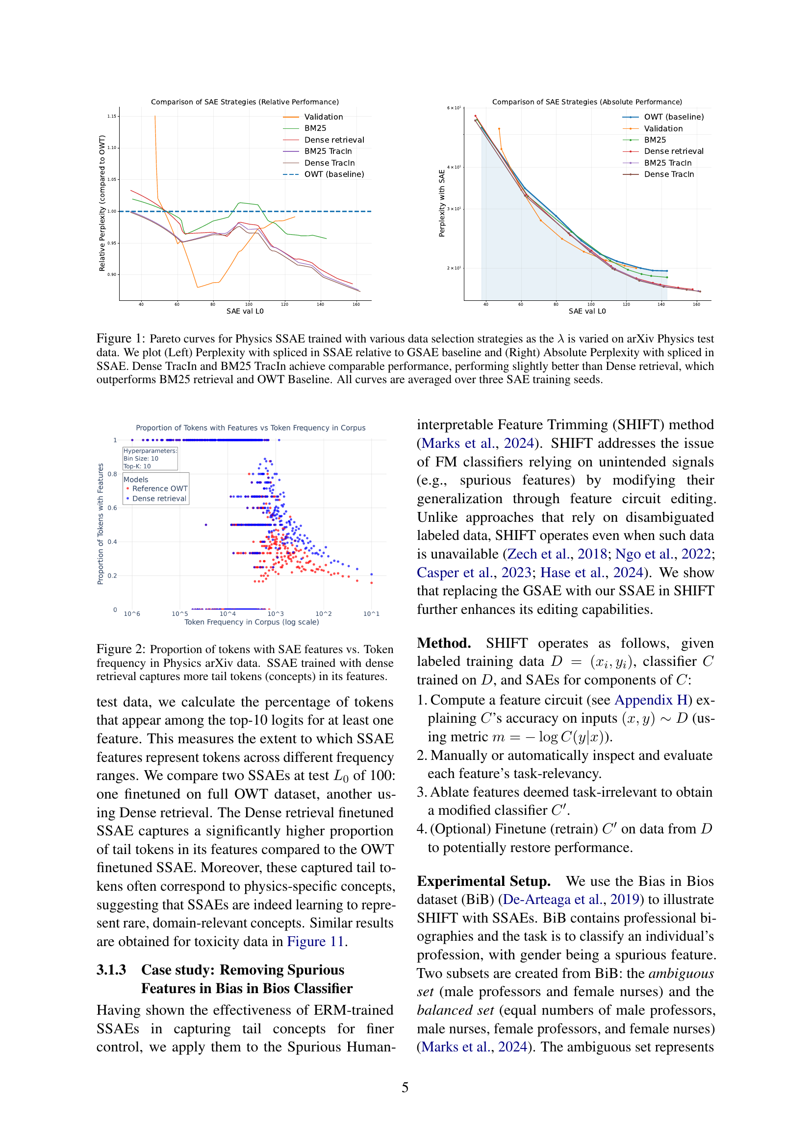
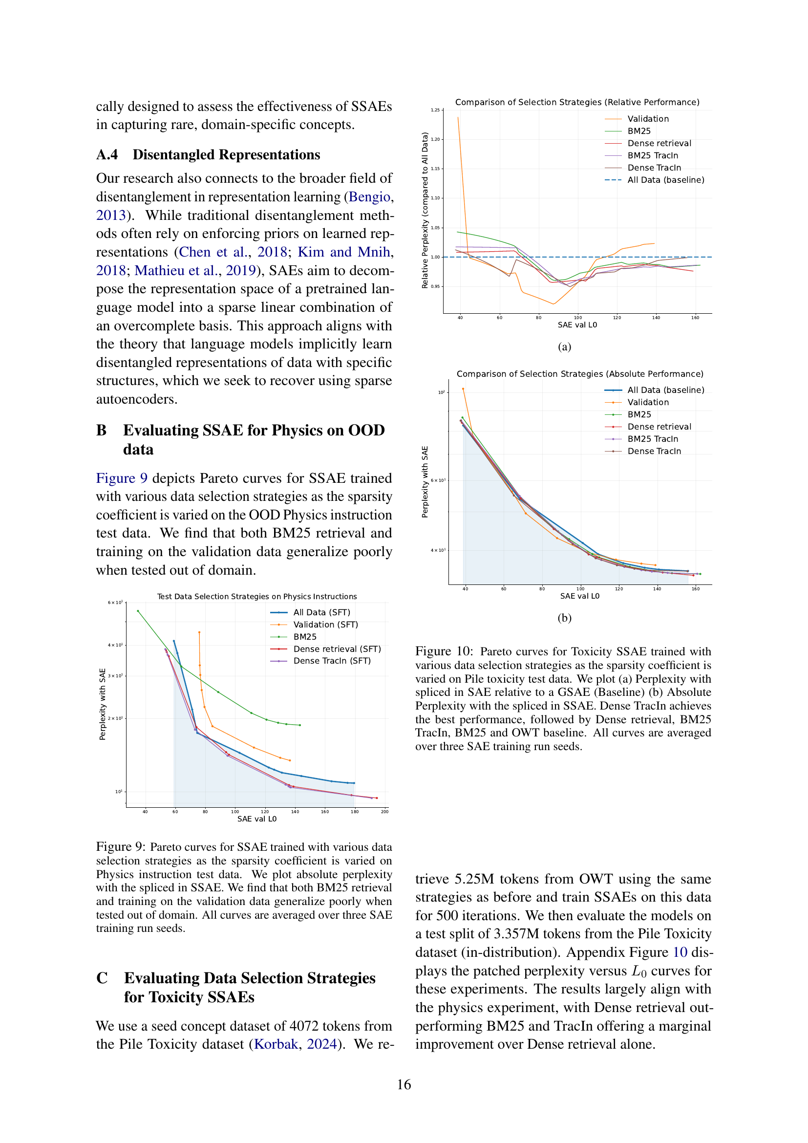
🔼 This figure displays the performance of Sparse Autoencoders (SAEs) trained using different data selection strategies on a physics dataset. Two key metrics are shown: perplexity (a measure of how well the SAE reconstructs the original data) and Lo sparsity (the average number of active features used in reconstruction). The left panel shows the relative perplexity compared to a general-purpose SAE baseline, while the right panel shows the absolute perplexity. The results indicate that using a combination of dense retrieval and TracIn reranking for data selection yields the best performance, slightly outperforming dense retrieval alone, which in turn is superior to BM25 retrieval and a baseline SAE trained on the full dataset. The curves represent the average of three separate training runs for each data selection strategy.
read the caption
Figure 1: Pareto curves for Physics SSAE trained with various data selection strategies as the λ𝜆\lambdaitalic_λ is varied on arXiv Physics test data. We plot (Left) Perplexity with spliced in SSAE relative to GSAE baseline and (Right) Absolute Perplexity with spliced in SSAE. Dense TracIn and BM25 TracIn achieve comparable performance, performing slightly better than Dense retrieval, which outperforms BM25 retrieval and OWT Baseline. All curves are averaged over three SAE training seeds.

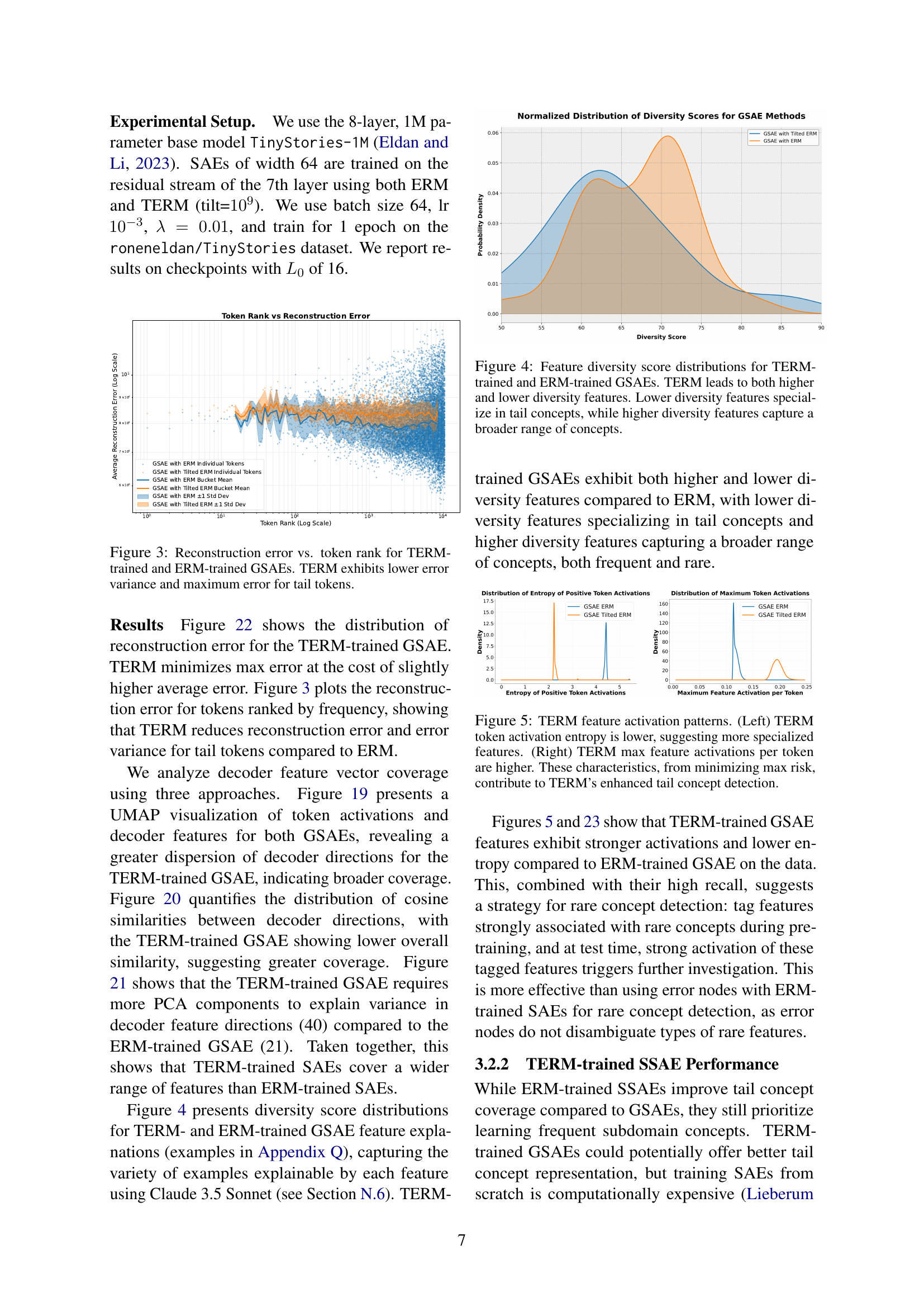
Method	↑Prof.	↓Gen.	↑Worst
Original	61.9	87.4	24.4
CBP	83.3	60.1	67.7
Neuron skyline	75.5	73.2	41.5
GSAE SHIFT	88.5	54.0	76.0
SSAE SHIFT	90.2	53.4	88.5
GSAE SHIFT+retrain	93.1	52.0	89.0
SSAE SHIFT+retrain	93.4	51.9	89.5
Comp. GSAE SHIFT	80.5	68.2	48.6
Comp. SSAE SHIFT	89.6	52.2	78.8
Comp. GSAE SHIFT+retrain	80.0	68.8	57.1
Comp. SSAE SHIFT+retrain	93.2	52.1	88.5
Oracle	93.0	49.4	91.9

🔼 This table presents the classification accuracy results on the Bias in Bios dataset for predicting professional roles while controlling for gender bias. It compares different methods for mitigating spurious correlations: original classifier, concept bottleneck probing (CBP), neuron skyline, and sparse autoencoder (SAE)-based SHIFT methods. The metrics include overall profession accuracy, gender accuracy, and worst-group accuracy (the lowest accuracy among the four subgroups: male professors, male nurses, female professors, female nurses). The table also shows results for compressed SAEs and the impact of retraining after feature removal. The best-performing method within each category is highlighted in bold.
read the caption
Table 1: Balanced set accuracies for intended (profession) and unintended (gender) labels. Worst refers to lowest profession accuracy among male professors, male nurses, female professors, and female nurses. Comp.: Compressed SAE (sliced to 1/8th width). Best results per method category are bolded.

In-depth insights
#

Rare Concept SAE
#

The research explores Specialized Sparse Autoencoders (SSAEs) to address the limitations of standard Sparse Autoencoders (SAEs) in capturing rare concepts within foundation models. SSAEs enhance the identification of these elusive ‘dark matter’ features by focusing on specific subdomains, rather than attempting global concept extraction. The methodology involves a practical recipe for training SSAEs, including dense retrieval for efficient data selection from a larger corpus and Tilted Empirical Risk Minimization (TERM) to improve the recall of tail concepts. Evaluation on standard metrics demonstrates SSAEs’ effectiveness in capturing subdomain-specific tail features and outperforming standard SAEs. A case study showcases their utility in removing spurious information, highlighting the potential of SSAEs as powerful tools for interpreting and mitigating risks associated with foundation models.

Subdomain Data Key
#

The research paper section ‘Subdomain Data Key’ is crucial for training effective Specialized Sparse Autoencoders (SSAEs). It highlights the importance of carefully selecting data relevant to the target subdomain for optimal performance. The paper proposes several data selection strategies, including sparse retrieval methods (like Okapi BM25) and dense retrieval techniques (like Contriever), which are used to expand small seed datasets by identifying relevant examples from a larger corpus. The choice of strategy and the subsequent data processing steps significantly influence the SSAE’s ability to capture rare, subdomain-specific features. Furthermore, reranking strategies like TracIn, which weighs data points based on their impact on model training, are explored to further refine the dataset and enhance the interpretability of learned features. The quality of the subdomain data plays a crucial role in the SSAE’s success, ultimately determining how effectively it isolates and represents infrequent concepts.

TERM Improves Recall
#

The section ‘TERM Improves Recall’ explores how Tilted Empirical Risk Minimization (TERM) enhances the ability of Sparse Autoencoders (SAEs) to capture rare concepts, addressing a key limitation of standard ERM training. TERM shifts the training objective from minimizing average loss to minimizing maximum risk, effectively forcing the SAE to pay more attention to tail concepts which are often overlooked. This results in improved recall, meaning more rare features are represented within the SAE’s learned representation. The authors demonstrate empirically that TERM-trained SSAEs (Specialized Sparse Autoencoders) achieve significantly better performance in capturing subdomain-specific tail concepts compared to ERM-trained SAEs. This improvement is particularly valuable in applications like AI safety, where identifying rare but potentially critical features is crucial. Furthermore, the results suggest that TERM may lead to more interpretable models, as the more balanced representation of both frequent and rare features fostered by TERM helps improve the understanding of the model’s inner workings.

Bias Mitigation Case
#

The Bias Mitigation Case study uses the Bias in Bios dataset to demonstrate how Specialized Sparse Autoencoders (SSAEs), trained with a Tilted Empirical Risk Minimization (TERM) objective, effectively remove spurious gender information. SSAEs outperform standard SAEs by achieving a 12.5% increase in worst-group classification accuracy when used to remove this spurious information. This improvement highlights the ability of SSAEs to identify and address rare, subdomain-specific features like gender bias, which standard SAEs often miss, thus advancing fairness and mitigating biases in foundation models. The effectiveness stems from the TERM-based training which focuses on minimizing the maximum risk, resulting in a better representation of rare and underrepresented concepts.

Future Work
#

The authors propose several avenues for future research, focusing on improving the computational efficiency of the Tilted Empirical Risk Minimization (TERM) training objective, which, while effective, is currently more computationally expensive than standard Empirical Risk Minimization (ERM). They suggest investigating alternative optimization strategies to make TERM more practical for wider adoption. Addressing the dependence of Specialized Sparse Autoencoders (SSAEs) on seed data quality is another key area, emphasizing the need for robust methods for automatically selecting high-quality seeds. Finally, they highlight the importance of rigorous generalization testing across more diverse domains and tasks, particularly in safety-critical applications, to fully evaluate the capabilities and limitations of SSAEs in enhancing interpretability and tail concept capture.

More visual insights
#

More on figures

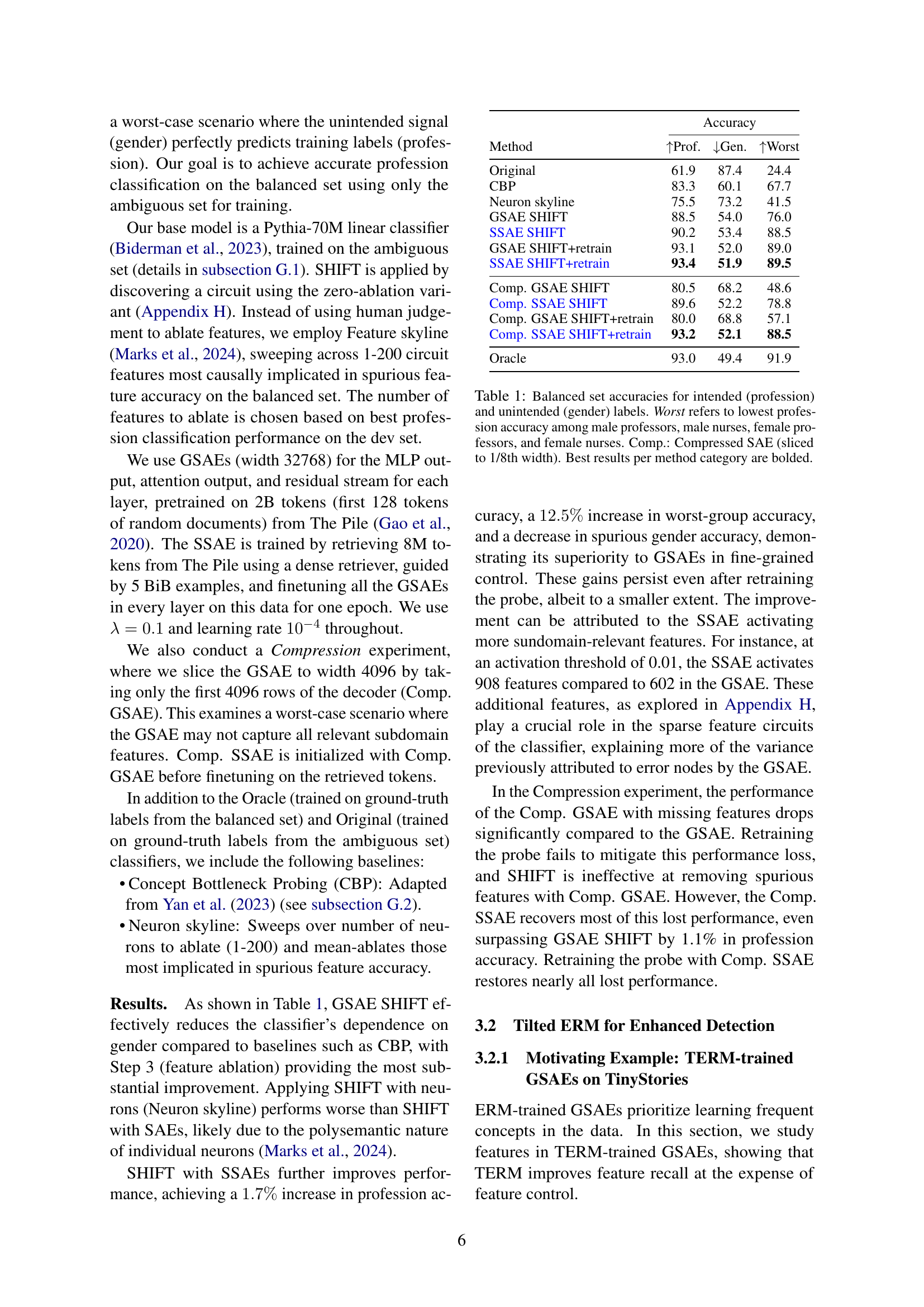
🔼 This figure shows the relationship between the frequency of tokens (words or sub-word units) in the Physics arXiv dataset and the proportion of those tokens that are represented by features in a Sparse Autoencoder (SAE). The x-axis represents the frequency of tokens (log scale), indicating how often each token appears in the dataset. The y-axis represents the proportion of tokens of a given frequency that are encoded by at least one feature in the SAE. A higher proportion indicates that the SAE effectively captures rarer tokens (tail concepts). The key finding is that an SAE trained using a dense retrieval method for data selection (SSAE) shows a noticeably higher proportion of tail tokens represented in its features compared to an SAE trained on general data, demonstrating its ability to capture rare concepts effectively.
read the caption
Figure 2: Proportion of tokens with SAE features vs. Token frequency in Physics arXiv data. SSAE trained with dense retrieval captures more tail tokens (concepts) in its features.

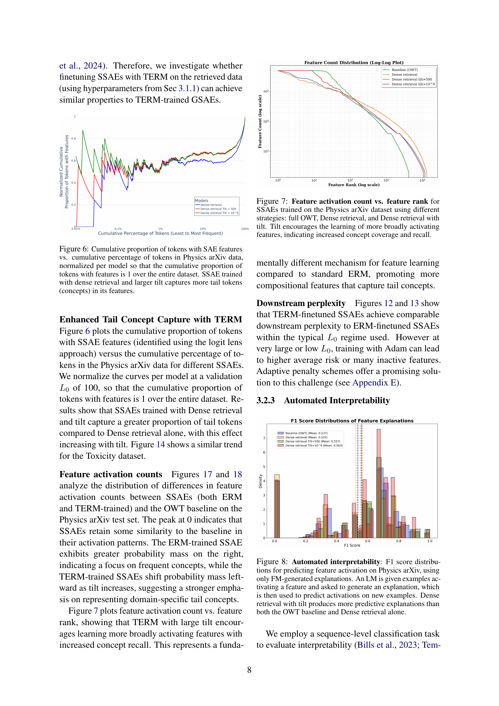
🔼 This figure compares the reconstruction error of tokens ranked by frequency for models trained with Tilted Empirical Risk Minimization (TERM) and standard Empirical Risk Minimization (ERM). The x-axis represents token rank (from most frequent to least frequent), and the y-axis shows the reconstruction error. The plot demonstrates that the TERM-trained model achieves lower average reconstruction error and significantly lower maximum reconstruction error for low-frequency (tail) tokens compared to the ERM-trained model, indicating improved performance and robustness for less common concepts.
read the caption
Figure 3: Reconstruction error vs. token rank for TERM-trained and ERM-trained GSAEs. TERM exhibits lower error variance and maximum error for tail tokens.

🔼 This figure shows the distributions of diversity scores for features extracted using Sparse Autoencoders (SAEs) trained with two different methods: Empirical Risk Minimization (ERM) and Tilted Empirical Risk Minimization (TERM). The diversity score measures the range of concepts a feature represents. The figure demonstrates that TERM leads to a wider range of feature diversity. Some TERM-trained SAE features are highly specific, focusing on rare concepts (tail concepts), while others are more general, covering a broader range of concepts. In contrast, ERM tends to produce features with intermediate diversity, not specializing in either tail concepts or broadly encompassing ones. This visualization highlights the effect of TERM in improving the representation of both frequent and infrequent concepts within the SAE feature space.
read the caption
Figure 4: Feature diversity score distributions for TERM-trained and ERM-trained GSAEs. TERM leads to both higher and lower diversity features. Lower diversity features specialize in tail concepts, while higher diversity features capture a broader range of concepts.

🔼 This figure displays the effect of Tilted Empirical Risk Minimization (TERM) on the distribution of Sparse Autoencoder (SAE) features. The left panel shows the entropy of token activations, demonstrating that TERM leads to lower entropy, implying more specialized features focused on individual concepts. The right panel shows the maximum activation value per token, indicating that TERM results in higher maximum activations. This combination of lower entropy and higher maximum activation suggests that TERM effectively prioritizes learning rarer features. In essence, TERM improves the ability of the model to learn and represent less frequent, yet potentially important, concepts.
read the caption
Figure 5: TERM feature activation patterns. (Left) TERM token activation entropy is lower, suggesting more specialized features. (Right) TERM max feature activations per token are higher. These characteristics, from minimizing max risk, contribute to TERM’s enhanced tail concept detection.

🔼 This figure shows the cumulative distribution of tokens with features identified by Sparse Autoencoders (SAEs) against the cumulative distribution of token frequencies in the Physics arXiv dataset. Each curve is normalized so that the cumulative proportion of tokens with features sums to 1 across the entire dataset, enabling direct comparison of coverage across different SAE training methods. The results demonstrate that SAEs trained using the Dense Retrieval method with a higher tilt parameter capture a greater proportion of tail tokens (those with lower frequencies), indicating their effectiveness in identifying rare concepts within the dataset.
read the caption
Figure 6: Cumulative proportion of tokens with SAE features vs. cumulative percentage of tokens in Physics arXiv data, normalized per model so that the cumulative proportion of tokens with features is 1 over the entire dataset. SSAE trained with dense retrieval and larger tilt captures more tail tokens (concepts) in its features.

🔼 This figure presents Pareto curves illustrating the trade-off between sparsity (measured by L0) and perplexity for Sparse Autoencoders (SAEs) trained using different data selection strategies on the Physics arXiv dataset. The strategies include training on the full OpenWebText corpus, using Dense Retrieval to select subdomain-relevant data, and employing Dense Retrieval in conjunction with a tilt parameter for Tilted Empirical Risk Minimization (TERM). The plot demonstrates that using Dense Retrieval with TERM (i.e., applying tilt) results in SAEs that learn features which activate more broadly across the dataset, compared to the other strategies. This increased breadth of activation is indicative of enhanced concept coverage and recall. By using TERM, the model focuses on minimizing the maximum loss rather than the average loss, which encourages it to capture rarer, less frequent concepts.
read the caption
Figure 7: Feature activation count vs. feature rank for SSAEs trained on the Physics arXiv dataset using different strategies: full OWT, Dense retrieval, and Dense retrieval with tilt. Tilt encourages the learning of more broadly activating features, indicating increased concept coverage and recall.

🔼 This figure displays the F1 scores achieved when using language model generated explanations to predict feature activation in a physics model. The x-axis represents the F1 score (a measure of prediction accuracy), and the y-axis represents the probability density, showing how often a given F1 score was obtained. The results are presented for different training methods: a baseline model trained on a general-purpose dataset (OWT), a model trained using dense retrieval, and a model trained using dense retrieval with a tilt parameter. The figure demonstrates that the model trained using dense retrieval with a tilt parameter produces significantly more accurate predictions (higher F1 score) compared to models trained using other methods. This is evidence of improved interpretability through this particular training technique.
read the caption
Figure 8: Automated interpretability: F1 score distributions for predicting feature activation on Physics arXiv, using only FM-generated explanations. An LM is given examples activating a feature and asked to generate an explanation, which is then used to predict activations on new examples. Dense retrieval with tilt produces more predictive explanations than both the OWT baseline and Dense retrieval alone.

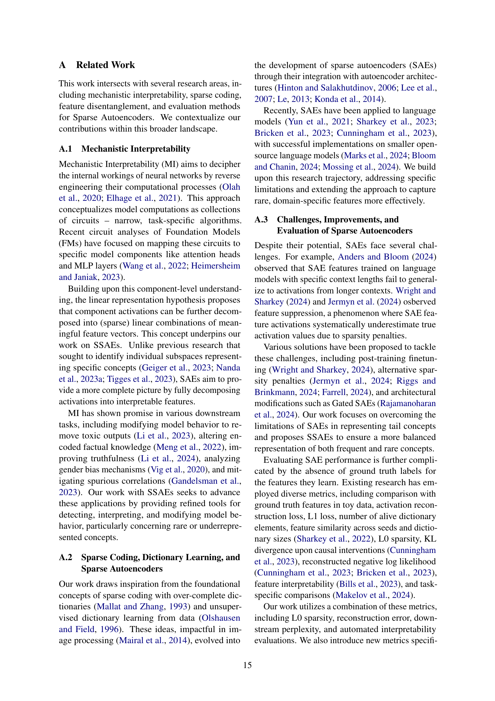
🔼 This figure displays Pareto curves, which show the trade-off between sparsity and reconstruction error, for Sparse Autoencoders (SAEs) trained using different data selection strategies. The x-axis represents the average number of active features (sparsity), and the y-axis represents the perplexity (a measure of reconstruction error) when the SAE’s reconstruction is used in a language model. The different curves represent SAEs trained with different methods for selecting training data: BM25 retrieval, Dense Retrieval, BM25 TracIn, Dense TracIn, and using the full dataset. The results show that training the SAE on a carefully curated dataset (using TracIn for example) leads to better generalization performance when compared to models trained using only the validation data or the full dataset. The poor performance when tested outside of the training data distribution (out-of-domain) highlights the importance of effective data selection for achieving robust and reliable SAEs.
read the caption
Figure 9: Pareto curves for SSAE trained with various data selection strategies as the sparsity coefficient is varied on Physics instruction test data. We plot absolute perplexity with the spliced in SSAE. We find that both BM25 retrieval and training on the validation data generalize poorly when tested out of domain. All curves are averaged over three SAE training run seeds.

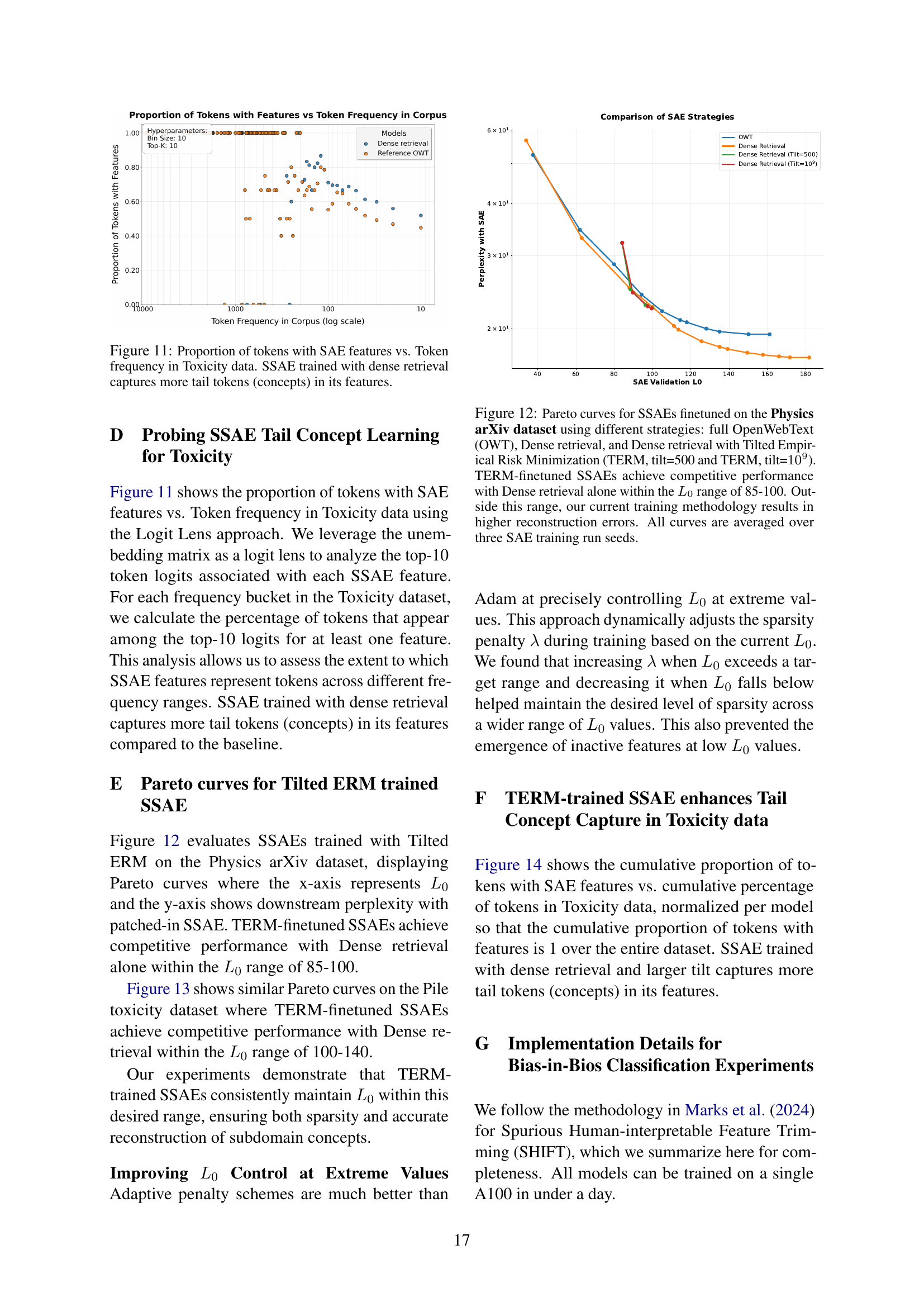
🔼 This figure shows the relationship between the frequency of tokens (words or sub-word units) in a toxicity dataset and the proportion of those tokens that are represented by features in a Sparse Autoencoder (SAE). The x-axis represents the frequency of tokens, while the y-axis shows the percentage of tokens with a given frequency that are encoded by at least one feature in the SAE. A higher value on the y-axis at lower token frequencies indicates better representation of rare (tail) concepts in the dataset. The results show that an SAE trained with a dense retrieval method (which helps to focus on relevant subdomain data) is able to capture a greater proportion of these rare tokens compared to a standard SAE trained on general data, confirming the effectiveness of this specialized approach for interpreting rare concepts.
read the caption
Figure 11: Proportion of tokens with SAE features vs. Token frequency in Toxicity data. SSAE trained with dense retrieval captures more tail tokens (concepts) in its features.

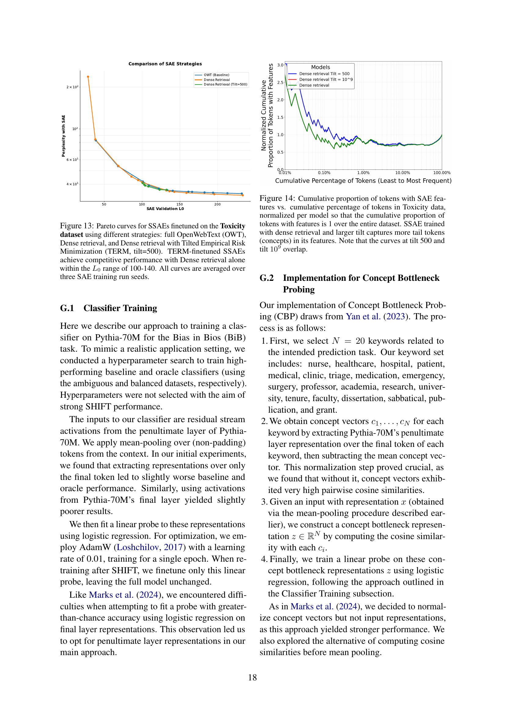
🔼 This figure displays Pareto curves illustrating the trade-off between sparsity (L0) and perplexity for Sparse Autoencoders (SAEs) fine-tuned on a physics dataset. Different data selection strategies are compared: using the entire OpenWebText corpus (OWT), using dense retrieval, and using dense retrieval combined with Tilted Empirical Risk Minimization (TERM) at tilt values of 500 and 10⁹. The results show that SAEs trained with TERM achieve performance comparable to dense retrieval alone within a specific L0 range (85-100). Outside this range, reconstruction errors increase, indicating limitations of the current training approach. The curves are averages across multiple runs to increase reliability.
read the caption
Figure 12: Pareto curves for SSAEs finetuned on the Physics arXiv dataset using different strategies: full OpenWebText (OWT), Dense retrieval, and Dense retrieval with Tilted Empirical Risk Minimization (TERM, tilt=500 and TERM, tilt=109superscript10910^{9}10 start_POSTSUPERSCRIPT 9 end_POSTSUPERSCRIPT). TERM-finetuned SSAEs achieve competitive performance with Dense retrieval alone within the L0subscript𝐿0L_{0}italic_L start_POSTSUBSCRIPT 0 end_POSTSUBSCRIPT range of 85-100. Outside this range, our current training methodology results in higher reconstruction errors. All curves are averaged over three SAE training run seeds.

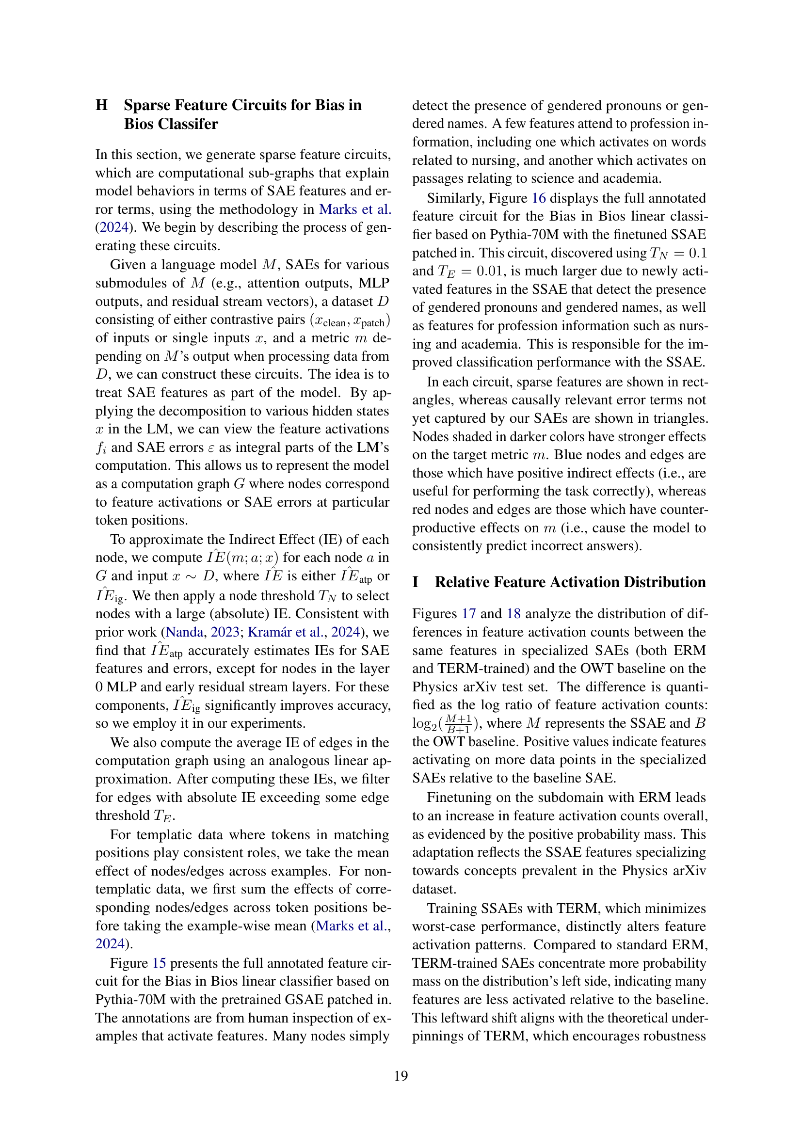
🔼 This figure presents Pareto curves illustrating the trade-off between sparsity (L0) and reconstruction error (perplexity) for Sparse Autoencoders (SAEs) fine-tuned on the Pile Toxicity dataset. Different data selection strategies were employed for training the SAEs: using the full OpenWebText corpus (OWT), using dense retrieval to select relevant data, and using dense retrieval combined with Tilted Empirical Risk Minimization (TERM) at a tilt of 500. The Pareto curves show that SAEs trained with dense retrieval and TERM achieve comparable performance to those trained with dense retrieval alone but only within a specific range of sparsity levels (L0 between 100 and 140). The results are averaged over multiple runs to provide a robust comparison.
read the caption
Figure 13: Pareto curves for SSAEs finetuned on the Toxicity dataset using different strategies: full OpenWebText (OWT), Dense retrieval, and Dense retrieval with Tilted Empirical Risk Minimization (TERM, tilt=500). TERM-finetuned SSAEs achieve competitive performance with Dense retrieval alone within the L0subscript𝐿0L_{0}italic_L start_POSTSUBSCRIPT 0 end_POSTSUBSCRIPT range of 100-140. All curves are averaged over three SAE training run seeds.

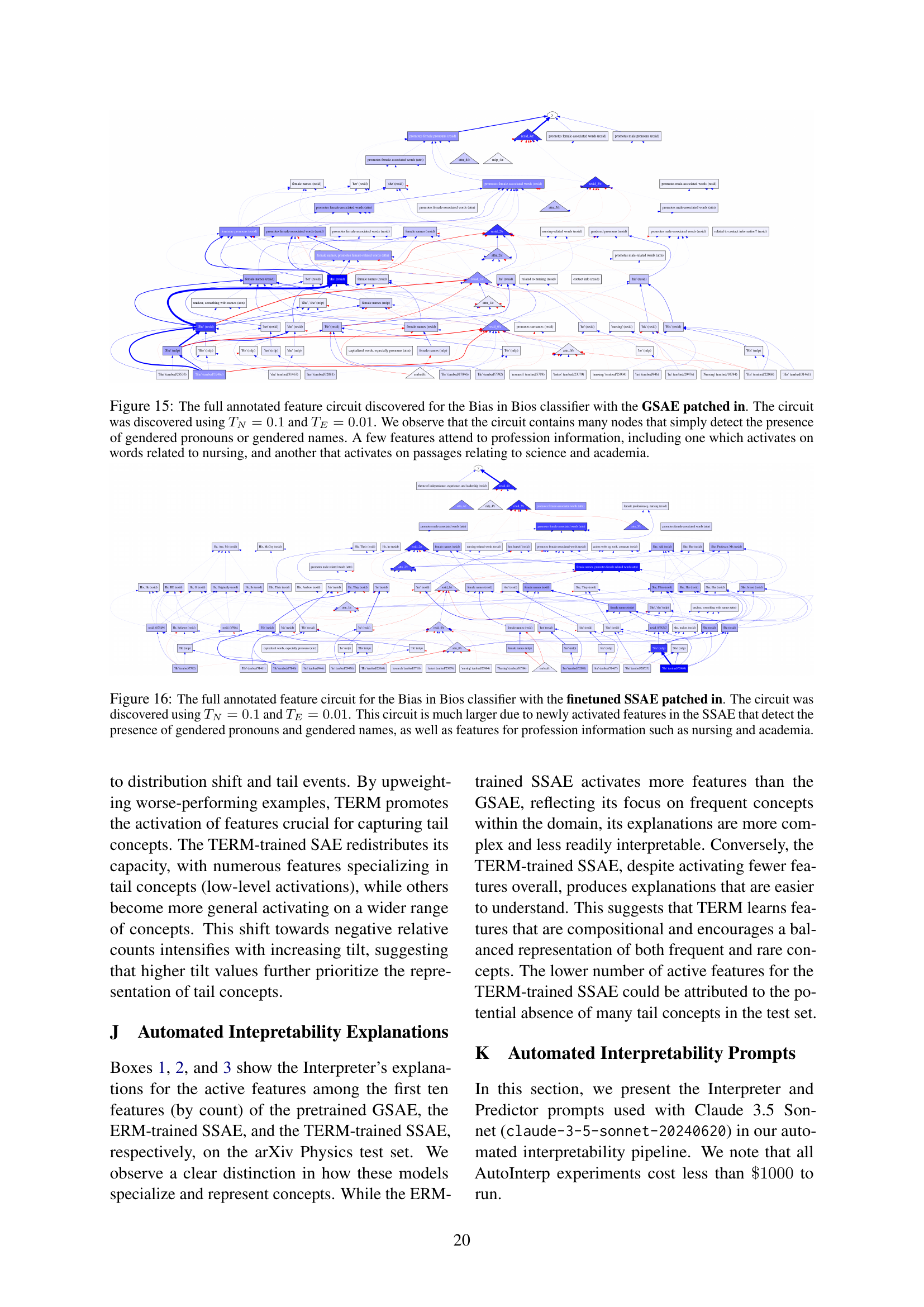
🔼 This figure shows the cumulative distribution of tokens with features extracted by Sparse Autoencoders (SAEs) compared to the cumulative distribution of token frequency in the Pile Toxicity dataset. The x-axis represents the cumulative percentage of tokens (from least to most frequent), and the y-axis represents the cumulative proportion of tokens having features according to the SAEs. Three different SAE training methods are shown: one trained on the entire dataset (baseline), one trained using dense retrieval of relevant tokens, and one trained using dense retrieval and the Tilted Empirical Risk Minimization (TERM) training objective with two different tilt parameters (500 and 10^9). The plot illustrates that SAEs trained with dense retrieval and TERM (especially with the higher tilt value) capture a significantly greater proportion of less frequent tokens (tail concepts) than the baseline SAE trained on the full dataset. The curves for the TERM models with tilt=500 and tilt=10^9 are nearly overlapping, suggesting that the improvement from increasing the tilt parameter beyond 500 may be marginal.
read the caption
Figure 14: Cumulative proportion of tokens with SAE features vs. cumulative percentage of tokens in Toxicity data, normalized per model so that the cumulative proportion of tokens with features is 1 over the entire dataset. SSAE trained with dense retrieval and larger tilt captures more tail tokens (concepts) in its features. Note that the curves at tilt 500 and tilt 109superscript10910^{9}10 start_POSTSUPERSCRIPT 9 end_POSTSUPERSCRIPT overlap.

🔼 This figure shows a sparse feature circuit, a graph illustrating the relationships between features extracted from a sparse autoencoder (SAE) and a model’s classification decisions, specifically for a bias detection task using the Bias in Bios dataset. The circuit highlights which SAE features are most influential in predicting whether a person is a nurse or a professor. It reveals that many features are focused on detecting gendered pronouns and names, indicating potential biases. However, some features do relate to the professions, for example, there is a feature for words related to nursing and another for words associated with science and academia.
read the caption
Figure 15: The full annotated feature circuit discovered for the Bias in Bios classifier with the GSAE patched in. The circuit was discovered using TN=0.1subscript𝑇𝑁0.1T_{N}=0.1italic_T start_POSTSUBSCRIPT italic_N end_POSTSUBSCRIPT = 0.1 and TE=0.01subscript𝑇𝐸0.01T_{E}=0.01italic_T start_POSTSUBSCRIPT italic_E end_POSTSUBSCRIPT = 0.01. We observe that the circuit contains many nodes that simply detect the presence of gendered pronouns or gendered names. A few features attend to profession information, including one which activates on words related to nursing, and another that activates on passages relating to science and academia.

🔼 This figure shows a feature circuit diagram for a Bias in Bios classifier. The classifier uses a Specialized Sparse Autoencoder (SSAE) which is a modified version of a standard Sparse Autoencoder (SAE) trained to focus on specific subdomains. The diagram visually represents how the SSAE’s features relate to the classifier’s predictions. Because it is trained on subdomains, it has many more activated features than the standard SAE. These features detect gendered pronouns, names, and profession-related terms such as ’nursing’ and ‘academia’. The circuit’s size is a consequence of the SSAE’s improved ability to capture rare concepts. The parameters T_N = 0.1 and T_E = 0.01 control the thresholds for node and edge selection, respectively.
read the caption
Figure 16: The full annotated feature circuit for the Bias in Bios classifier with the finetuned SSAE patched in. The circuit was discovered using TN=0.1subscript𝑇𝑁0.1T_{N}=0.1italic_T start_POSTSUBSCRIPT italic_N end_POSTSUBSCRIPT = 0.1 and TE=0.01subscript𝑇𝐸0.01T_{E}=0.01italic_T start_POSTSUBSCRIPT italic_E end_POSTSUBSCRIPT = 0.01. This circuit is much larger due to newly activated features in the SSAE that detect the presence of gendered pronouns and gendered names, as well as features for profession information such as nursing and academia.

🔼 This figure shows the distribution of differences in the number of times each feature was activated, comparing specialized sparse autoencoders (SAEs) trained with Empirical Risk Minimization (ERM) and Tilted Empirical Risk Minimization (TERM) against a general-purpose SAE. The x-axis represents the log-ratio of the feature activation counts in the specialized SAEs relative to the general-purpose SAE. Positive values indicate features more frequently activated in specialized SAEs. The distribution for the ERM-trained SAE is skewed right, signifying that it favors common concepts. In contrast, the distribution for the TERM-trained SAE is shifted to the left, indicating a stronger focus on less frequent, domain-specific concepts. This highlights how TERM helps SAEs capture rare concepts.
read the caption
Figure 17: Distribution of log-ratio feature activation count differences between specialized SAEs and the OWT baseline on the Physics arXiv test set, normalized per SAE model. Blue represents the ERM-trained SSAE with Dense retrieval, orange represents the TERM-trained SSAE with tilt=500. The ERM-trained SSAE exhibits more probability mass on the right, indicating an emphasis on representing common concepts, while the TERM-trained SSAE’s shift towards the left suggests a greater focus on representing domain-specific tail concepts.

🔼 Figure 18 shows the distribution of the difference in the number of times features are activated between specialized sparse autoencoders (SAEs) trained with empirical risk minimization (ERM) and tilted empirical risk minimization (TERM), and a general-purpose SAE. The data is from the arXiv Physics test set, and the results are normalized per SAE model. The blue curve represents ERM-trained SAEs using dense retrieval, while the orange curve shows TERM-trained SAEs with a tilt parameter of 10⁹. The plot demonstrates that TERM increasingly emphasizes rarer concepts (tail concepts) compared to ERM, which prioritizes more frequent concepts (head concepts). The greater leftward shift in the orange curve for TERM at tilt 10⁹ visually represents the increased focus on rarer concepts.
read the caption
Figure 18: Distribution of log-ratio feature activation count differences on the Physics arXiv test set, normalized per SAE model. Blue represents the ERM-trained SSAE with Dense retrieval, orange represents the TERM-trained SSAE with tilt=109superscript10910^{9}10 start_POSTSUPERSCRIPT 9 end_POSTSUPERSCRIPT. The intensified leftward shift of probability mass with higher tilt demonstrates that TERM increasingly prioritizes representing tail concepts compared to standard ERM-trained SSAE, which focuses more on frequent concepts.

🔼 This figure displays a UMAP visualization comparing the token activations and decoder directions learned by two types of Sparse Autoencoders (SAEs): one trained using standard Empirical Risk Minimization (ERM), and the other trained using Tilted Empirical Risk Minimization (TERM). The UMAP projection shows the decoder directions for the TERM-trained SAE are more spread out than those of the ERM-trained SAE. This indicates that the TERM-trained SAE has learned a more diverse set of features, covering a wider range of concepts and capturing more of the nuances in the data compared to the ERM-trained SAE. The wider spread of features suggests that TERM is more effective at capturing tail concepts (rare, infrequent features) that would be missed by a standard ERM-trained SAE.
read the caption
Figure 19: UMAP visualization of token activations and decoder features for a TERM-trained and ERM-trained GSAE. Decoder directions for TERM-trained GSAE appear more spread out, suggesting the SAE has wider coverage than the ERM-trained GSAE.

🔼 This figure displays the distribution of cosine similarity scores between the decoder directions learned by two different types of generative sparse autoencoders (GSAEs): one trained with Empirical Risk Minimization (ERM), and the other trained with Tilted Empirical Risk Minimization (TERM). The cosine similarity measures how similar the learned feature vectors are. A lower average cosine similarity indicates that the TERM-trained GSAE has learned more diverse and distinct feature directions, implying that it has captured a wider range of concepts from the data.
read the caption
Figure 20: Distribution of cosine similarities between decoder directions of TERM-trained and ERM-trained GSAEs. TERM-trained GSAE shows lower similarity between decoder feature directions implying greater coverage.

Feature	Explanation
h.7_feature3	Unified explanation: This neuron recognizes narrative structures in simple, moralistic children’s stories. It activates on new story segments, character introductions, settings, conflicts, and dialogue. Frequent themes include lessons on kindness, honesty, and sharing. Examples: 1. “Lily woke up early on Saturday morning. ‘Mom, can I go play with my friend Jenny?’ she asked.” 2. “Once upon a time, there was a little boy named Tommy who loved to play with his toys but never wanted to share.” 3. “After school, Timmy came home feeling sad. ‘What’s wrong?’ his mom asked. ‘I got in trouble for not telling the truth,’ Timmy replied.” Diversity Score: 71 Justification: Activates on diverse narrative elements in children’s stories, including dialogue, character introductions, settings, events, emotions, and moral lessons. High diversity within the genre of educational stories for young audiences.
h.7_feature5	Unified explanation: This neuron activates on language patterns associated with conveying moral lessons, advice, and guidance on appropriate behavior in children’s stories or parental scenarios. It frequently fires on modal verbs like “should” and “can” when characters are learning about right and wrong actions, facing consequences, or being instructed on proper conduct. Examples: 1. “You should not take things that don’t belong to you,” said Mom, after catching Timmy taking a candy bar from the store. 2. “The little boy learned that he can be kind to others by sharing his toys.” 3. “If you can’t say something nice, you should not say anything at all,” advised the teacher to the rowdy class. Diversity Score: 68 Justification: While specializing in moral lessons and guidance, the range of potential lessons, advice, and behavioral instructions is quite broad. It activates across various story elements and moral themes, encompassing a diverse array of instructional language in children’s literature.
h.7_feature6	Unified Explanation: This neuron activates when “<
h.7_feature12	Unified explanation: This neuron activates at the beginning of short stories or narratives aimed at children. The consistent trigger is the token “<

Feature	Explanation
h.7_feature8	Unified explanation: This feature detects the indefinite article “an” when introducing new or significant elements in children’s stories or simple narratives. It activates when “an” precedes a noun at the beginning of a sentence or clause, signaling a novel element important to the plot. Examples: 1. “An old man lived in a tiny house by the forest.” 2. “One day, an unexpected visitor arrived at the village.” 3. “Deep in the ocean, an ancient treasure awaited discovery.” Diversity Score: 65 Justification: High diversity in types of elements introduced (characters, objects, concepts) within children’s stories, but limited to narrative contexts.
h.7_feature13	Unified explanation: This feature captures interjections or exclamations in children’s stories or dialogues expressing surprise, excitement, or drawing attention to something noteworthy. Tokens like “Wow” or “Look” often appear at the beginning of quoted speech or exclamations. Examples: 1. “Wow! Look at that giant castle!” a child might exclaim upon seeing an impressive structure. 2. “Look, the caterpillar turned into a butterfly!” a character might say, pointing out a transformation. 3. “Wow, that was a close one!” someone might remark after narrowly avoiding danger. Diversity Score: 71 Justification: While specific to interjections, these can be used across a wide range of contexts and story elements, reflecting a high degree of diversity within children’s stories and dialogues.
h.7_feature14	Unified explanation: This neuron predicts words related to pleasant or appetizing food experiences in children’s stories or simple narratives. It activates on the first few letters of words like “yummy”, “candy”, “crumbs”, and “celery”, generating vocabulary associated with tasty treats, cooking, or domestic activities. Examples: 1. “The little girl licked her lips as she stared at the yummy chocolate cake.” 2. “After playing outside, the kids ran to the kitchen for a snack of celery and peanut butter.” 3. “Mom swept up the crumbs from the cookies the children had enjoyed earlier.” Diversity Score: 53 Justification: While primarily focused on food-related words, it recognizes a range of vocabulary including adjectives, nouns, and verbs related to food experiences in children’s stories.
h.7_feature17	Unified explanation: This neuron processes text related to children’s stories, simple narratives, and basic concepts in children’s literature. It responds to character names, diminutives, dialogue markers, sensory experiences, emotions, onomatopoeias, common objects, food items, childhood experiences, simple actions, and basic vocabulary. Examples: 1. “Ducky waddled over to the lollipop on the ground. ’Yum!’ he exclaimed, gobbling it up.” 2. “Ow, ow, ow! Timmy had scraped his knee on the rough sand. Mom kissed it better and gave him a sausage to cheer him up.” 3. “Bark, bark! Spidey’s new puppy was digging in the garden, scattering the soil everywhere. ’No, no, pup!’ scolded Spidey.” Diversity Score: 85 Justification: Displays very high diversity within children’s literature, responding to a wide range of elements including characters, emotions, actions, objects, sensory experiences, and dialogue patterns.

TL;DR#

Key Takeaways#

Why does it matter?#

Visual Insights#

In-depth insights#

Rare Concept SAE#

Subdomain Data Key#

TERM Improves Recall#

Bias Mitigation Case#

Future Work#

More visual insights#

Full paper#