↗ arXiv ↗ Hugging Face ↗ Papers with Code
TL;DR#
Autoregressive models have shown promise in image generation, but they often lag behind diffusion models due to their inherent unidirectional nature which is not ideal for visual data. Existing attempts to improve this by adding bidirectional attention often deviate from the traditional autoregressive paradigm, hindering their integration into unified multimodal models.
This paper introduces Randomized Autoregressive Modeling (RAR), a simple yet effective technique to enhance the performance of autoregressive image generation models without altering the core framework. RAR randomly permutes the input sequence during training, encouraging the model to learn from all possible factorization orders. This process, combined with a randomness annealing strategy, effectively improves bidirectional context modeling, leading to significant gains in image generation quality while maintaining compatibility with language modeling frameworks. The results show RAR outperforms state-of-the-art methods on the ImageNet-256 benchmark.
Key Takeaways#
Why does it matter?#
This paper is crucial because it significantly advances autoregressive visual generation, a vital area in computer vision. By introducing a novel training strategy, it achieves state-of-the-art results, surpassing both previous autoregressive and other leading methods. This opens avenues for research in unified multimodal models and scalable visual generation.
Visual Insights#

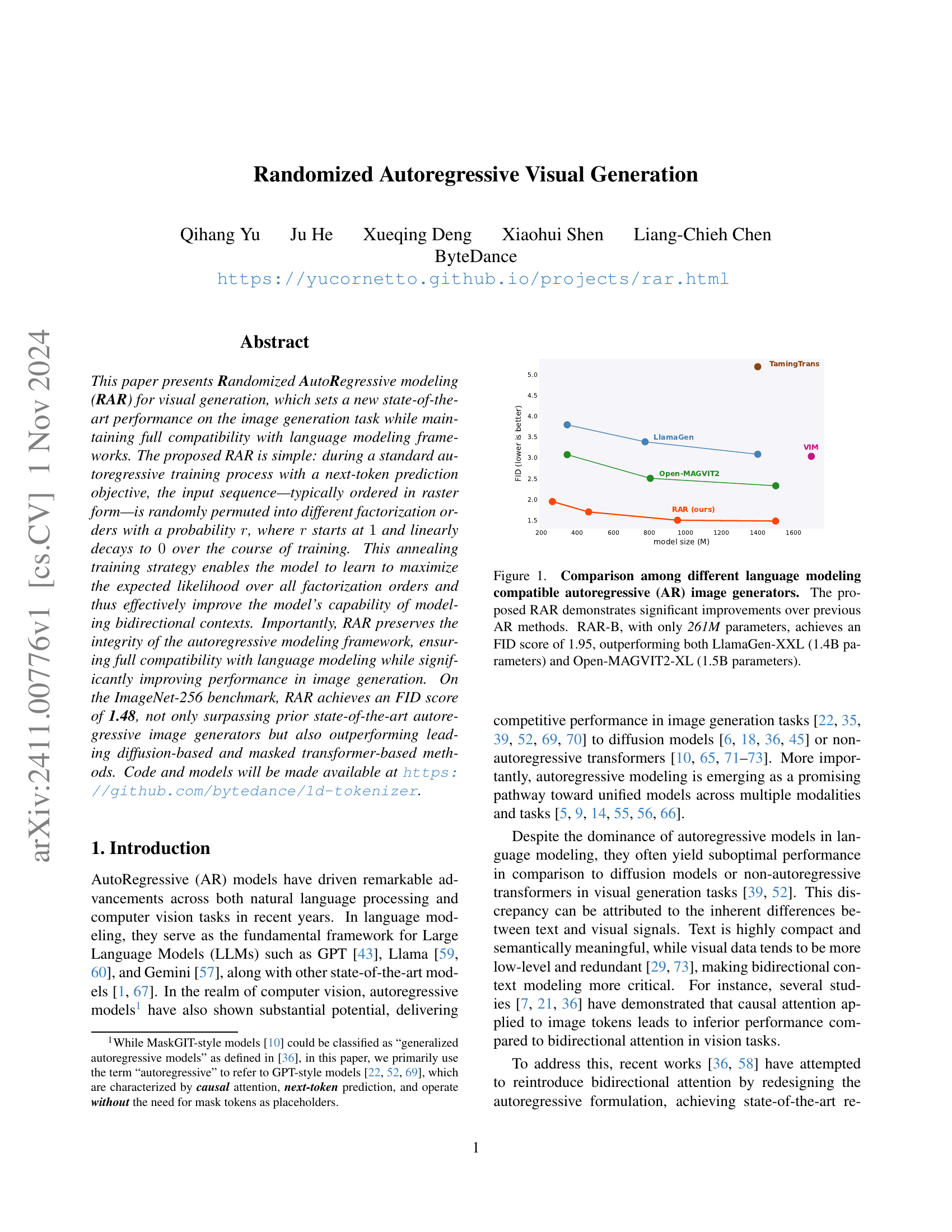
🔼 The figure shows a comparison of the Fréchet Inception Distance (FID) scores achieved by various autoregressive (AR) image generation models, including the proposed Randomized Autoregressive (RAR) model. Lower FID scores indicate better image quality. RAR-B, a smaller model with only 261 million parameters, achieves an FID of 1.95, outperforming significantly larger models like LlamaGen-XXL (1.4 billion parameters) and Open-MAGVIT2-XL (1.5 billion parameters). This highlights the effectiveness of RAR in improving image generation quality while maintaining compatibility with language modeling frameworks.
read the caption
Figure 1: Comparison among different language modeling compatible autoregressive (AR) image generators. The proposed RAR demonstrates significant improvements over previous AR methods. RAR-B, with only 261M parameters, achieves an FID score of 1.95, outperforming both LlamaGen-XXL (1.4B parameters) and Open-MAGVIT2-XL (1.5B parameters).
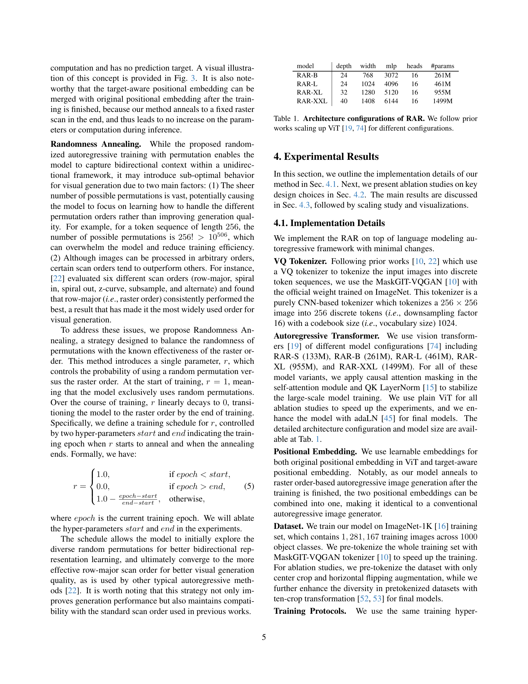
| model | depth | width | mlp | heads | #params |
|---|---|---|---|---|---|
| RAR-B | 24 | 768 | 3072 | 16 | 261M |
| RAR-L | 24 | 1024 | 4096 | 16 | 461M |
| RAR-XL | 32 | 1280 | 5120 | 16 | 955M |
| RAR-XXL | 40 | 1408 | 6144 | 16 | 1499M |
🔼 Table 1 details the different model architectures used in the Randomized Autoregressive visual generation experiments. It shows how the model’s depth, width, MLP size, and number of attention heads vary across four different configurations (RAR-B, RAR-L, RAR-XL, and RAR-XXL). These configurations are based on scaling up the Vision Transformer (ViT) architecture, following the approach used in prior research.
read the caption
Table 1: Architecture configurations of RAR. We follow prior works scaling up ViT [19, 74] for different configurations.
In-depth insights#
RAR: Bidirectional AR#
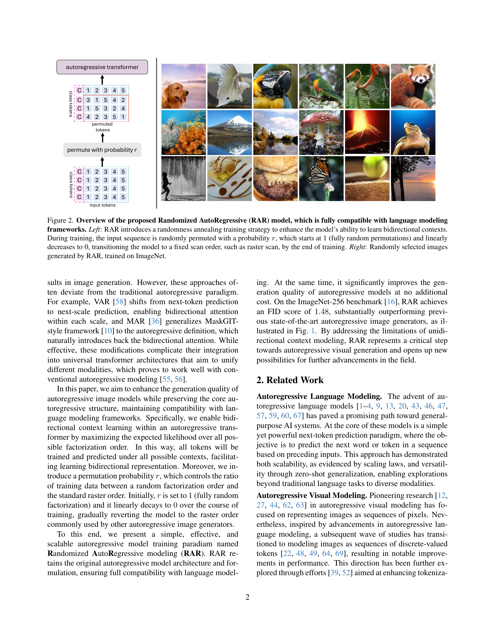
The research paper section ‘RAR: Bidirectional AR’ introduces Randomized Autoregressive Modeling (RAR), a novel approach to enhance autoregressive image generation. RAR addresses the limitations of unidirectional autoregressive models by introducing randomness during training. The input token sequence is randomly permuted with a probability r, which anneals from 1 (fully random) to 0 (raster scan) over training. This strategy forces the model to learn bidirectional contexts by maximizing the expected likelihood across all permutation orders. Importantly, RAR preserves the autoregressive framework, ensuring compatibility with language modeling while significantly boosting performance. The effectiveness is demonstrated through improved FID scores on ImageNet-256, surpassing existing autoregressive and diffusion-based methods. A key element is the introduction of target-aware positional embeddings, which guides the model during training with permuted sequences, addressing potential ambiguity in prediction.
Annealing Strategy#
The research paper introduces a novel randomness annealing strategy to enhance autoregressive image generation. This strategy involves a control parameter, r, that governs the probability of using random token order permutations during training. Initially, r is set to 1, employing entirely random permutations, enabling the model to learn bidirectional relationships between image tokens effectively. As training progresses, r linearly decays to 0, transitioning the model to the standard raster scan order. This annealing process is crucial; it starts by maximizing the model’s exposure to diverse context arrangements. The gradual shift to the raster scan helps ensure the model converges on an effective token order, preventing the random permutations from hindering the final model’s performance and facilitating compatibility with existing language modeling frameworks. This carefully controlled introduction of randomness ensures the model effectively learns rich bidirectional contexts without compromising overall training stability or generation quality. The results show that this strategy significantly enhances performance, demonstrating the power of controlled randomness in autoregressive visual modeling.
Positional Embeddings#
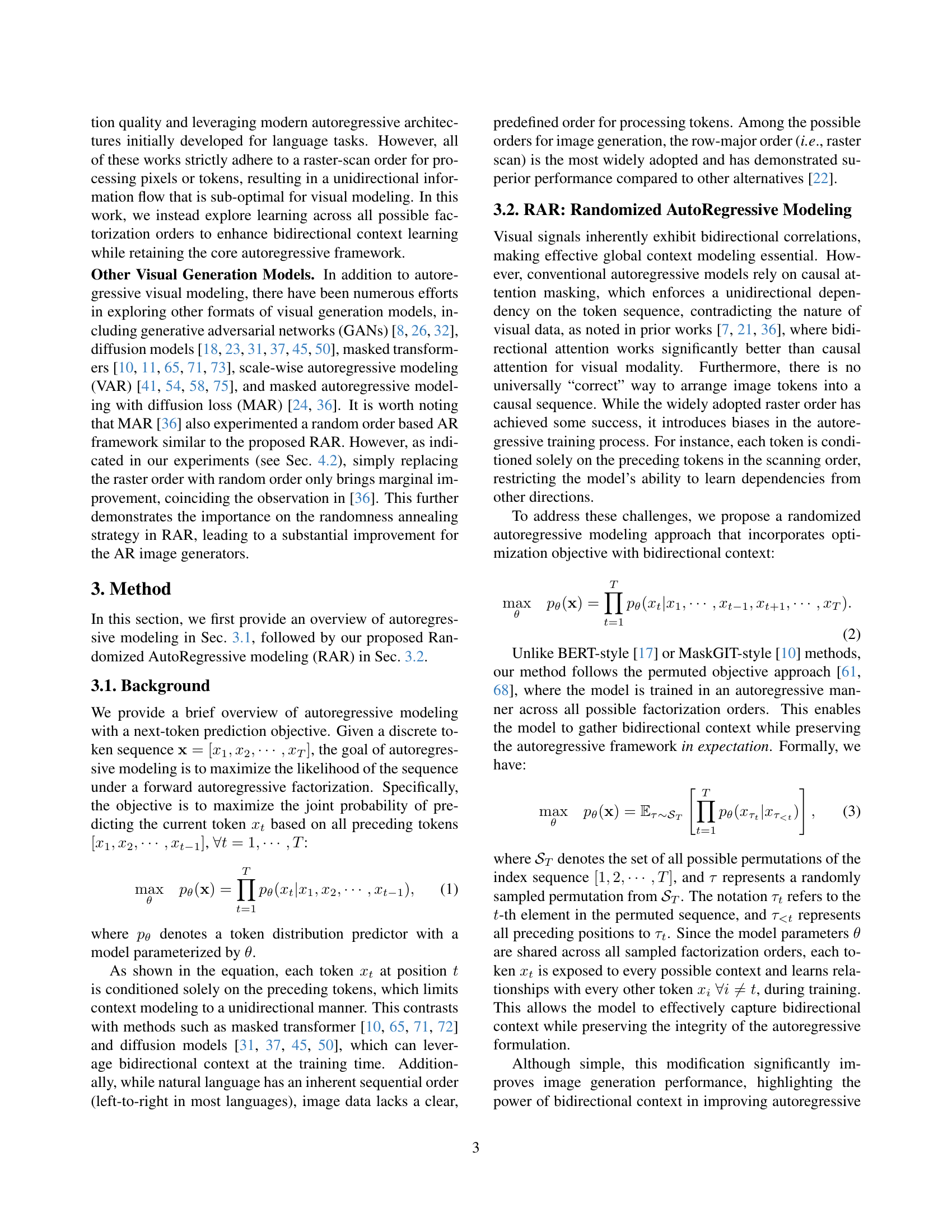
The research paper introduces target-aware positional embeddings to address limitations of standard positional embeddings within the randomized autoregressive framework. Standard positional embeddings can fail when identical prediction logits arise from different token permutations, hindering the model’s ability to learn from all possible factorization orders. Target-aware embeddings encode information about which token is being predicted next, resolving this ambiguity and ensuring each token prediction has access to the correct context. This enhancement significantly improves the model’s capability to learn bidirectional dependencies from randomly permuted image tokens during the training phase, ultimately boosting the overall image generation performance. The integration of target-aware positional embeddings is a crucial component that enables the successful use of a fully randomized training strategy while maintaining the compatibility of the core autoregressive framework with language models.
Ablation Studies#
The ablation studies section meticulously investigates the impact of key design choices within the RAR model. Randomness Annealing, a crucial component, is tested with varying start and end epochs for the randomness schedule, revealing its effectiveness in balancing exploration and exploitation. The impact of different scan orders on final model performance is also analyzed. Results reveal that while other orders yield reasonable performance, the standard raster scan order ultimately delivers superior results, aligning with established practice and providing a beneficial baseline. These experiments demonstrate the critical roles of the randomness annealing and the chosen scan order in achieving the model’s superior image generation quality and offer valuable insights into the design choices affecting this novel autoregressive visual generation model.
Future Works#
The authors outline several promising avenues for future research. Improving the handling of global context during generation is a primary goal, acknowledging that the current approach, while incorporating bidirectional information, still relies on a sequential generation process. They suggest exploring techniques like resampling or refinement to enhance context awareness. Extending the model’s versatility is another key area, implying work on diverse modalities or tasks beyond image generation, leveraging the model’s inherent compatibility with language modeling frameworks. Investigating alternative positional embedding strategies represents a further refinement to enhance the robustness and efficiency of the randomized approach, especially considering the complexity of handling various scan orders. Finally, in-depth analysis of the randomness annealing strategy and exploration of optimal parameter settings are envisioned, with the goal of enhancing training stability and generalization performance.
More visual insights#
More on figures

🔼 Figure 2 illustrates the Randomized Autoregressive (RAR) model, designed for visual generation while maintaining compatibility with language modeling frameworks. The left panel demonstrates the RAR training process: input sequences are randomly permuted with a probability r, initially 1 (fully random) and decreasing linearly to 0 during training. This annealing strategy helps the model learn bidirectional contexts by maximizing the likelihood across various permutation orders, eventually converging to a fixed raster scan. The right panel showcases example images generated by the trained RAR model using the ImageNet dataset.
read the caption
Figure 2: Overview of the proposed Randomized AutoRegressive (RAR) model, which is fully compatible with language modeling frameworks. Left: RAR introduces a randomness annealing training strategy to enhance the model’s ability to learn bidirectional contexts. During training, the input sequence is randomly permuted with a probability r𝑟ritalic_r, which starts at 1 (fully random permutations) and linearly decreases to 0, transitioning the model to a fixed scan order, such as raster scan, by the end of training. Right: Randomly selected images generated by RAR, trained on ImageNet.

🔼 Figure 3 illustrates the concept of target-aware positional embeddings within the Randomized Autoregressive (RAR) model. Panel (a) depicts the training process: images are first tokenized into patches (following the Vision Transformer architecture), each patch receiving an initial positional embedding (blue tokens). The token sequence is then randomly permuted. Crucially, a target-aware positional embedding (green tokens) is added to each token to inform the model which token it should predict next. Panels (b) and (c) showcase the importance of these target-aware embeddings. Panel (b) shows a failure scenario where, without them, two different permuted sequences produce identical predictions because the original positional embeddings alone aren’t sufficient to distinguish the correct prediction in the context of a random permutation. Panel (c) demonstrates that the inclusion of target-aware positional embeddings successfully guides the model toward the correct next-token prediction, even with a randomly permuted input sequence.
read the caption
Figure 3: Illustration of the target-aware positional embedding. Subfigure (a) shows the training process of the proposed Randomized AutoRegressive (RAR) model, along with the target-aware position embedding. Following Vision Transformer [19], images are tokenized into patches with original position embeddings (blue tokens). The token sequence is then randomly permuted, with the target-aware positional embeddings (green tokens) added to guide the model. Subfigures (b) and (c) highlight the importance of the target-aware positional embedding: (b) demonstrates a failure case where both permuted sequences yield identical prediction logits, while (c) shows that the target-aware positional embedding correctly guides the model to predict the next token accurately.

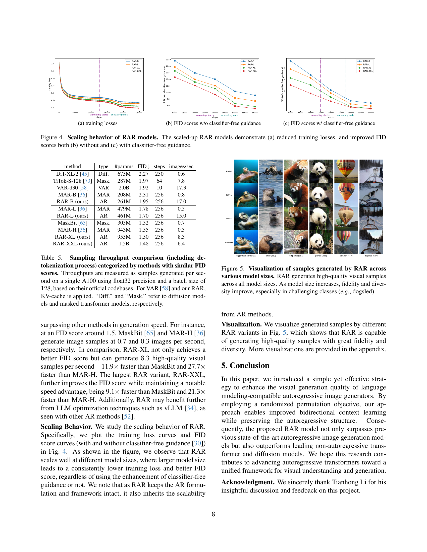
🔼 This figure shows the scaling behavior of the RAR model across different sizes (RAR-B, RAR-L, RAR-XL, RAR-XXL). Subfigure (a) presents the training loss curves for each model variant over training steps. Subfigures (b) and (c) illustrate the FID scores (a metric evaluating image generation quality) with and without classifier-free guidance, respectively. The plots demonstrate how larger models generally achieve lower training losses and better FID scores.
read the caption
(a) training losses

🔼 This figure shows the FID scores achieved by different sized RAR models (RAR-B, RAR-L, RAR-XL, RAR-XXL) without using classifier-free guidance during training. The x-axis represents the training steps, showing the FID score progression over the training process. Different lines represent the FID for each model size. The purpose is to demonstrate the impact of model size on the FID score and assess how well the model generalizes.
read the caption
(b) FID scores w/o classifier-free guidance

🔼 This figure shows the FID (Fréchet Inception Distance) scores achieved by different sized RAR models (RAR-B, RAR-L, RAR-XL, RAR-XXL) when using classifier-free guidance during training. Lower FID scores indicate better image generation quality. The x-axis represents the training steps, showing the progress over the training period. The plot demonstrates the improvement in FID score as model size increases and the effectiveness of classifier-free guidance in enhancing the image generation capabilities of the RAR models.
read the caption
(c) FID scores w/ classifier-free guidance

🔼 This figure analyzes the scaling behavior of the Randomized Autoregressive (RAR) model across different sizes. Subfigure (a) shows that as the model size increases, the training loss decreases, indicating improved model training efficiency. Subfigures (b) and (c) present the Fréchet Inception Distance (FID) scores, a metric for evaluating image quality, with and without classifier-free guidance, respectively. Both subfigures show that larger RAR models consistently achieve lower FID scores, demonstrating that scaling up the model significantly improves the image quality generated.
read the caption
Figure 4: Scaling behavior of RAR models. The scaled-up RAR models demonstrate (a) reduced training losses, and improved FID scores both (b) without and (c) with classifier-free guidance.

🔼 This figure displays example images generated by the RAR model at different scales (RAR-B, RAR-L, RAR-XL, and RAR-XXL). The images demonstrate the model’s ability to generate high-quality images across all model sizes. Notably, as the model size increases, the fidelity and diversity of the generated images improve. This improvement is particularly evident in complex or challenging classes, such as the example of a ‘dogsled’ which contains many fine details and multiple objects.
read the caption
Figure 5: Visualization of samples generated by RAR across various model sizes. RAR generates high-quality visual samples across all model sizes. As model size increases, fidelity and diversity improve, especially in challenging classes (e.g., dogsled).

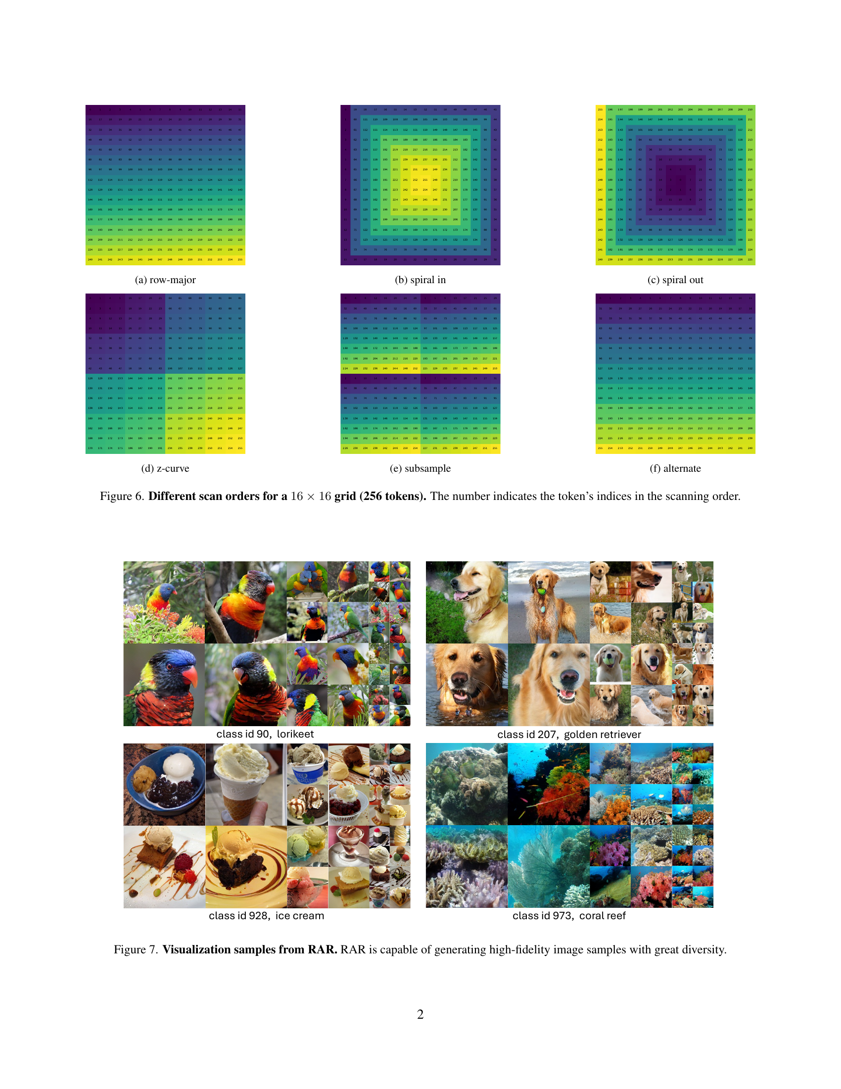
🔼 This figure visualizes six different scan orders for a 16x16 grid (256 tokens). Each subfigure displays one scan order, showing the order in which tokens are processed. The numbers within each grid represent the index of the token according to that scan order. The scan orders visualized are row-major, spiral in, spiral out, z-curve, subsample, and alternate.
read the caption
(a) row-major

🔼 This subfigure shows one of the six different scan orders tested in the paper for image generation. The spiral scan order starts from the center of the image and spirals outwards, processing pixels in a circular pattern. The numbers in the image indicate the sequence in which each token (representing a pixel or a patch of pixels) is processed. This visualization helps illustrate how different scan orders affect the order of information received by the autoregressive model during training and generation.
read the caption
(b) spiral in

🔼 This figure is a visualization of one of six different scan orders used for processing a 16x16 image (256 tokens) within an autoregressive model. Specifically, it showcases the ‘spiral out’ scan order, where the tokens are processed in a spiral pattern, starting from the center and expanding outwards. The numbers in each cell represent the order in which the tokens are processed.
read the caption
(c) spiral out

🔼 This subfigure shows a visualization of the ‘z-curve’ scan order for a 16x16 grid (256 tokens). A z-curve is a space-filling curve that traverses a grid in a pattern resembling the letter ‘Z’. This particular visualization displays the order in which the tokens are processed, with each number representing the index of the token in the scan order.
read the caption
(d) z-curve

🔼 This image shows a visualization of the ‘subsample’ scan order for a 16x16 grid (256 tokens). The numbers represent the order in which the tokens are processed. Unlike a raster scan which would process tokens sequentially, row by row, this subsampling pattern skips tokens in a specific way. The pattern is designed to demonstrate an alternative autoregressive factorization of the image data, which is explored in the paper as a method to improve context modeling.
read the caption
(e) subsample

🔼 This figure visualizes one of the six different scan orders evaluated in the paper for autoregressive image generation. The alternate scan order processes the image tokens in an alternating pattern across rows, starting from the top left, then moving to the second row from the left, and so on. The numbers represent the order in which the tokens are scanned.
read the caption
(f) alternate

🔼 Figure 6 visualizes six different ways of scanning a 16x16 grid (256 tokens), representing different orders for processing image data in an autoregressive model. Each scan order is displayed as a grid where the numbers indicate the order in which the model processes the tokens. This illustrates the impact of different scan orders on how the model learns and generates images, particularly focusing on the tradeoff between unidirectional (raster scan) and bidirectional (randomized scan) processing of the image. The visualization is directly relevant to the exploration of how the model’s ability to learn and utilize bidirectional context is affected by different factorization orders of the image data during training. The figure is important to show the impact on model learning as the various scanning approaches in the ablation study can significantly impact the model’s learning of contextual information in the model.
read the caption
Figure 6: Different scan orders for a 16×16161616\times 1616 × 16 grid (256 tokens). The number indicates the token’s indices in the scanning order.

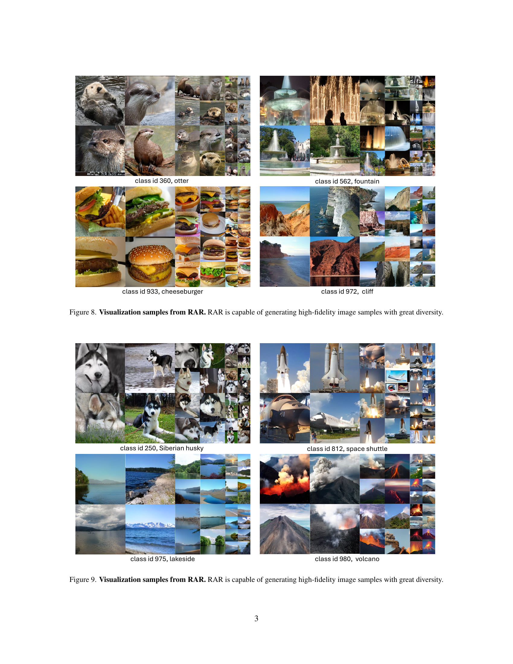
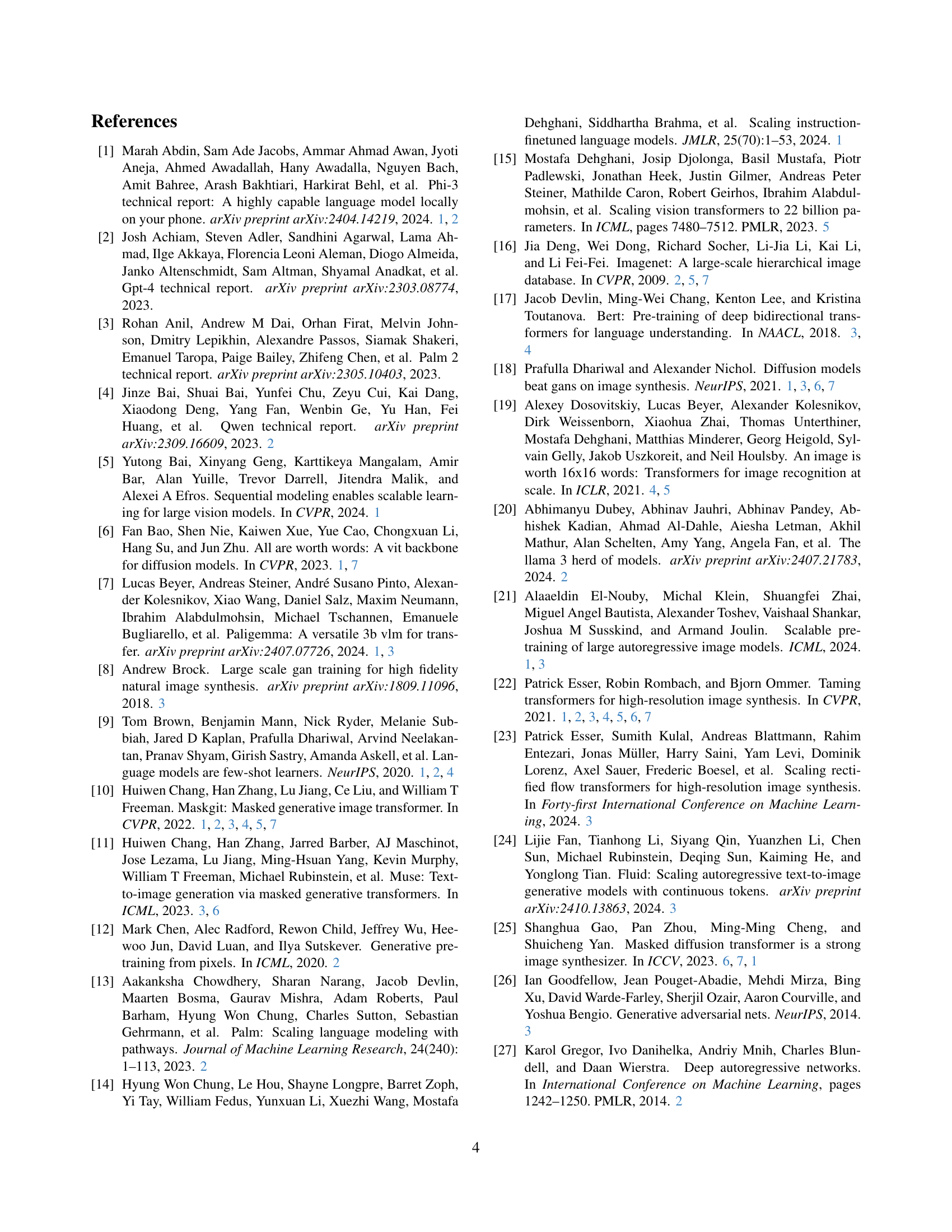
🔼 Figure 7 showcases a diverse set of images generated by the Randomized Autoregressive (RAR) model. The images demonstrate the model’s ability to generate high-quality, detailed, and visually diverse samples across a wide range of classes and object characteristics, highlighting its strong performance in image generation.
read the caption
Figure 7: Visualization samples from RAR. RAR is capable of generating high-fidelity image samples with great diversity.
More on tables
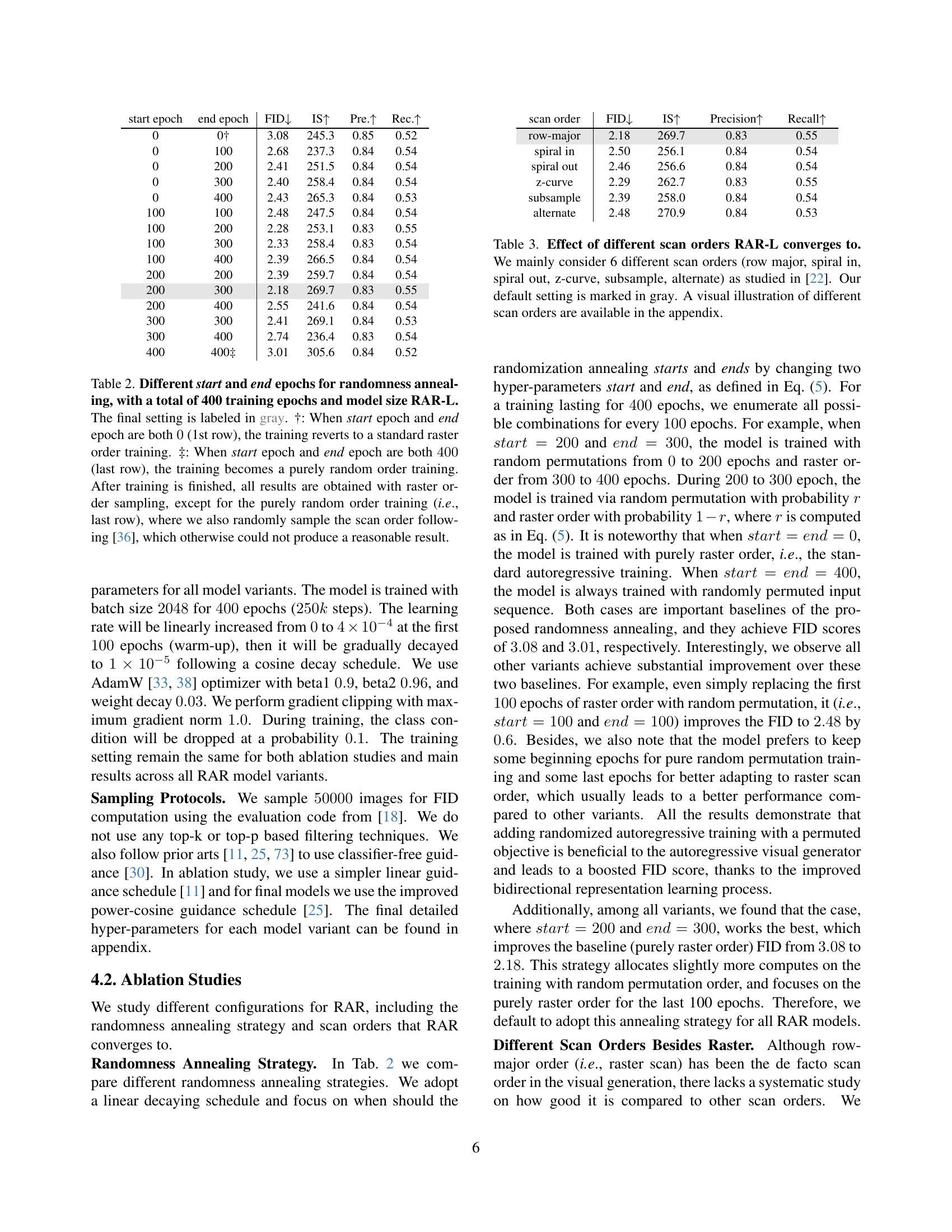
| start epoch | end epoch | FID ↓ | IS ↑ | Pre. ↑ | Rec. ↑ |
|---|---|---|---|---|---|
| 0 | 0† | 3.08 | 245.3 | 0.85 | 0.52 |
| 0 | 100 | 2.68 | 237.3 | 0.84 | 0.54 |
| 0 | 200 | 2.41 | 251.5 | 0.84 | 0.54 |
| 0 | 300 | 2.40 | 258.4 | 0.84 | 0.54 |
| 0 | 400 | 2.43 | 265.3 | 0.84 | 0.53 |
| 100 | 100 | 2.48 | 247.5 | 0.84 | 0.54 |
| 100 | 200 | 2.28 | 253.1 | 0.83 | 0.55 |
| 100 | 300 | 2.33 | 258.4 | 0.83 | 0.54 |
| 100 | 400 | 2.39 | 266.5 | 0.84 | 0.54 |
| 200 | 200 | 2.39 | 259.7 | 0.84 | 0.54 |
| 200 | 300 | 2.18 | 269.7 | 0.83 | 0.55 |
| 200 | 400 | 2.55 | 241.6 | 0.84 | 0.54 |
| 300 | 300 | 2.41 | 269.1 | 0.84 | 0.53 |
| 300 | 400 | 2.74 | 236.4 | 0.83 | 0.54 |
| 400 | 400‡ | 3.01 | 305.6 | 0.84 | 0.52 |
🔼 This table presents an ablation study on the randomness annealing strategy used in the RAR model. It shows the impact of varying the start and end epochs of the annealing process on the model’s performance, as measured by FID, IS, Precision, and Recall. The total number of training epochs is fixed at 400. The first row represents training with a purely raster scan order, while the last row shows results from training with purely random scan orders. The gray row indicates the chosen configuration used in the rest of the paper. The table also highlights the importance of the gradual transition between purely random to raster order in the annealing process.
read the caption
Table 2: Different start and end epochs for randomness annealing, with a total of 400 training epochs and model size RAR-L. The final setting is labeled in gray. †: When start epoch and end epoch are both 00 (1st row), the training reverts to a standard raster order training. ‡: When start epoch and end epoch are both 400400400400 (last row), the training becomes a purely random order training. After training is finished, all results are obtained with raster order sampling, except for the purely random order training (i.e., last row), where we also randomly sample the scan order following [36], which otherwise could not produce a reasonable result.
| scan order | FID ↓ | IS ↑ | Precision ↑ | Recall ↑ |
|---|---|---|---|---|
| row-major | 2.18 | 269.7 | 0.83 | 0.55 |
| spiral in | 2.50 | 256.1 | 0.84 | 0.54 |
| spiral out | 2.46 | 256.6 | 0.84 | 0.54 |
| z-curve | 2.29 | 262.7 | 0.83 | 0.55 |
| subsample | 2.39 | 258.0 | 0.84 | 0.54 |
| alternate | 2.48 | 270.9 | 0.84 | 0.53 |
🔼 This table investigates the impact of different image scanning orders on the performance of the RAR-L model. Six common scan orders, including the standard row-major order, are compared. The results show the final FID, Inception Score (IS), precision, and recall after training with each scan order. The default settings used in the experiments are highlighted in gray for easy reference. A visual representation of each scan order is provided in the appendix for better understanding.
read the caption
Table 3: Effect of different scan orders RAR-L converges to. We mainly consider 6 different scan orders (row major, spiral in, spiral out, z-curve, subsample, alternate) as studied in [22]. Our default setting is marked in gray. A visual illustration of different scan orders are available in the appendix.
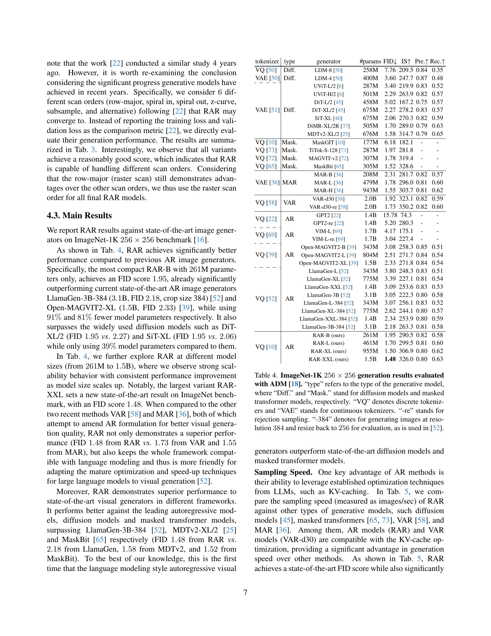
| tokenizer | type | generator | #params | FID ↓ | IS ↑ | Pre. ↑ | Rec. ↑ |
|---|---|---|---|---|---|---|---|
| VQ [50] | Diff. | LDM-8 [50] | 258M | 7.76 | 209.5 | 0.84 | 0.35 |
| VAE [50] | Diff. | LDM-4 [50] | 400M | 3.60 | 247.7 | 0.87 | 0.48 |
| VAE [51] | Diff. | UViT-L/2 [6] | 287M | 3.40 | 219.9 | 0.83 | 0.52 |
| UViT-H/2 [6] | 501M | 2.29 | 263.9 | 0.82 | 0.57 | ||
| DiT-L/2 [45] | 458M | 5.02 | 167.2 | 0.75 | 0.57 | ||
| DiT-XL/2 [45] | 675M | 2.27 | 278.2 | 0.83 | 0.57 | ||
| SiT-XL [40] | 675M | 2.06 | 270.3 | 0.82 | 0.59 | ||
| DiMR-XL/2R [37] | 505M | 1.70 | 289.0 | 0.79 | 0.63 | ||
| MDTv2-XL/2 [25] | 676M | 1.58 | 314.7 | 0.79 | 0.65 | ||
| VQ [10] | Mask. | MaskGIT [10] | 177M | 6.18 | 182.1 | - | - |
| VQ [73] | Mask. | TiTok-S-128 [73] | 287M | 1.97 | 281.8 | - | - |
| VQ [72] | Mask. | MAGVIT-v2 [72] | 307M | 1.78 | 319.4 | - | - |
| VQ [65] | Mask. | MaskBit [65] | 305M | 1.52 | 328.6 | - | - |
| VAE [36] | MAR | MAR-B [36] | 208M | 2.31 | 281.7 | 0.82 | 0.57 |
| MAR-L [36] | 479M | 1.78 | 296.0 | 0.81 | 0.60 | ||
| MAR-H [36] | 943M | 1.55 | 303.7 | 0.81 | 0.62 | ||
| VQ [58] | VAR | VAR-d30 [58] | 2.0B | 1.92 | 323.1 | 0.82 | 0.59 |
| VAR-d30-re [58] | 2.0B | 1.73 | 350.2 | 0.82 | 0.60 | ||
| VQ [22] | AR | GPT2 [22] | 1.4B | 15.78 | 74.3 | - | - |
| GPT2-re [22] | 1.4B | 5.20 | 280.3 | - | - | ||
| VQ [69] | AR | VIM-L [69] | 1.7B | 4.17 | 175.1 | - | - |
| VIM-L-re [69] | 1.7B | 3.04 | 227.4 | - | - | ||
| VQ [39] | AR | Open-MAGVIT2-B [39] | 343M | 3.08 | 258.3 | 0.85 | 0.51 |
| Open-MAGVIT2-L [39] | 804M | 2.51 | 271.7 | 0.84 | 0.54 | ||
| Open-MAGVIT2-XL [39] | 1.5B | 2.33 | 271.8 | 0.84 | 0.54 | ||
| VQ [52] | AR | LlamaGen-L [52] | 343M | 3.80 | 248.3 | 0.83 | 0.51 |
| LlamaGen-XL [52] | 775M | 3.39 | 227.1 | 0.81 | 0.54 | ||
| LlamaGen-XXL [52] | 1.4B | 3.09 | 253.6 | 0.83 | 0.53 | ||
| LlamaGen-3B [52] | 3.1B | 3.05 | 222.3 | 0.80 | 0.58 | ||
| LlamaGen-L-384 [52] | 343M | 3.07 | 256.1 | 0.83 | 0.52 | ||
| LlamaGen-XL-384 [52] | 775M | 2.62 | 244.1 | 0.80 | 0.57 | ||
| LlamaGen-XXL-384 [52] | 1.4B | 2.34 | 253.9 | 0.80 | 0.59 | ||
| LlamaGen-3B-384 [52] | 3.1B | 2.18 | 263.3 | 0.81 | 0.58 | ||
| VQ [10] | AR | RAR-B (ours) | 261M | 1.95 | 290.5 | 0.82 | 0.58 |
| RAR-L (ours) | 461M | 1.70 | 299.5 | 0.81 | 0.60 | ||
| RAR-XL (ours) | 955M | 1.50 | 306.9 | 0.80 | 0.62 | ||
| RAR-XXL (ours) | 1.5B | 1.48 | 326.0 | 0.80 | 0.63 |
🔼 Table 4 presents a comparison of various image generation models on the ImageNet-1K dataset, focusing on 256x256 image generation. The models are categorized by type (diffusion, masked transformer, autoregressive), tokenizer type (discrete VQ or continuous VAE), and whether rejection sampling was used. Results are evaluated using the Fréchet Inception Distance (FID) metric, with additional metrics provided in some cases. Note that some models generate images at a resolution of 384x384 and then resize to 256x256 for consistent evaluation.
read the caption
Table 4: ImageNet-1K 256×256256256256\times 256256 × 256 generation results evaluated with ADM [18]. “type” refers to the type of the generative model, where “Diff.” and “Mask.” stand for diffusion models and masked transformer models, respectively. “VQ” denotes discrete tokenizers and “VAE” stands for continuous tokenizers. “-re” stands for rejection sampling. “-384” denotes for generating images at resolution 384384384384 and resize back to 256256256256 for evaluation, as is used in [52].
| method | type | #params | FID ↓ | steps | images/sec |
|---|---|---|---|---|---|
| DiT-XL/2 [45] | Diff. | 675M | 2.27 | 250 | 0.6 |
| TiTok-S-128 [73] | Mask. | 287M | 1.97 | 64 | 7.8 |
| VAR-d30 [58] | VAR | 2.0B | 1.92 | 10 | 17.3 |
| MAR-B [36] | MAR | 208M | 2.31 | 256 | 0.8 |
| RAR-B (ours) | AR | 261M | 1.95 | 256 | 17.0 |
| MAR-L [36] | MAR | 479M | 1.78 | 256 | 0.5 |
| RAR-L (ours) | AR | 461M | 1.70 | 256 | 15.0 |
| MaskBit [65] | Mask. | 305M | 1.52 | 256 | 0.7 |
| MAR-H [36] | MAR | 943M | 1.55 | 256 | 0.3 |
| RAR-XL (ours) | AR | 955M | 1.50 | 256 | 8.3 |
| RAR-XXL (ours) | AR | 1.5B | 1.48 | 256 | 6.4 |
🔼 This table compares the speed of generating images (samples/second) using different image generation models on a single NVIDIA A100 GPU. The models are grouped based on their Fréchet Inception Distance (FID) scores, a metric indicating image quality, to ensure a fair comparison. The throughput is measured using float32 precision and a batch size of 128, following the original codebases of each method. Notably, the models using autoregressive architectures (RAR and VAR) utilize KV-cache optimization for efficiency, resulting in higher speeds. ‘Diff.’ indicates diffusion models and ‘Mask.’ represents masked transformer models. The table highlights how the proposed RAR method is not only efficient in generating images but also significantly faster than many other methods with comparable FID scores.
read the caption
Table 5: Sampling throughput comparison (including de-tokenization process) categorized by methods with similar FID scores. Throughputs are measured as samples generated per second on a single A100 using float32 precision and a batch size of 128128128128, based on their official codebases. For VAR [58] and our RAR, KV-cache is applied. “Diff.” and “Mask.” refer to diffusion models and masked transformer models, respectively.
| config | value |
|---|---|
| training hyper-params | |
| optimizer | AdamW [33, 38] |
| learning rate | 4e-4 |
| weight decay | 0.03 |
| optimizer momentum | (0.9, 0.96) |
| batch size | 2048 |
| learning rate schedule | cosine decay |
| ending learning rate | 1e-5 |
| total epochs | 400 |
| warmup epochs | 100 |
| annealing start epoch | 200 |
| annealing end epoch | 300 |
| precision | bfloat16 |
| max grad norm | 1.0 |
| dropout rate | 0.1 |
| attn dropout rate | 0.1 |
| class label dropout rate | 0.1 |
| sampling hyper-params | |
| guidance schedule | pow-cosine [25] |
| temperature | 1.0 (B) / 1.02 (L, XL, XXL) |
| scale power | 2.75 (B) / 2.5 (L) / 1.5 (XL) / 1.2 (XXL) |
| guidance scale | 16.0 (B) / 15.5 (L) / 6.9 (XL) / 8.0 (XXL) |
🔼 Table 6 presents the detailed hyperparameter settings used for training the final versions of the Randomized Autoregressive (RAR) models. These settings encompass both training hyperparameters (optimizer, learning rate, weight decay, batch size, learning rate schedule, etc.) and sampling hyperparameters (temperature, scale power, and guidance scale), offering a comprehensive overview of the configuration employed to achieve the reported results. The table is broken down into two sections, one for training and one for sampling, which provides clarity in understanding the various parameters.
read the caption
Table 6: Detailed hyper-parameters for final RAR models.
Full paper#
