↗ arXiv ↗ Hugging Face ↗ Papers with Code
TL;DR#
Large language models (LLMs) often contain many weakly-contributing elements in their activation outputs. Reducing these improves efficiency and interpretability. However, existing research lacks a comprehensive understanding of the factors influencing activation sparsity. This paper investigates this gap by focusing on decoder-only Transformer-based LLMs.
The researchers propose a new metric, PPL-p% sparsity, to precisely measure activation sparsity while considering model performance. Through extensive experiments, they uncover several scaling laws describing the relationship between activation sparsity and training data, activation functions, and architectural design. These findings provide valuable insights into designing LLMs with significantly greater activation sparsity, ultimately paving the way towards more efficient and interpretable AI.
Key Takeaways#
Why does it matter?#
This paper is crucial because it provides practical, quantifiable guidelines for designing more efficient and interpretable LLMs. It introduces novel empirical laws governing activation sparsity, impacting LLM optimization and potentially accelerating future research on efficient model architectures. This work’s findings could drastically improve the speed and interpretability of LLMs, leading to significant advancements in various AI applications.
Visual Insights#

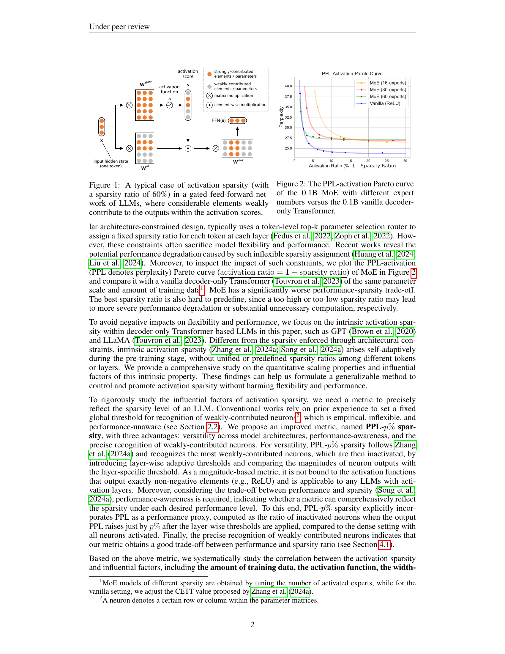
🔼 Figure 1 illustrates activation sparsity in a large language model (LLM). The gated feed-forward network within the LLM processes input, and the activation function produces an output. In this example, a significant portion (60%) of the activation function’s output consists of elements with weak contributions to the final output. These weakly-contributing elements represent the activation sparsity, and they can be eliminated for potential computational gains or model interpretation improvements.
read the caption
Figure 1: A typical case of activation sparsity (with a sparsity ratio of 60%) in a gated feed-forward network of LLMs, where considerable elements weakly contribute to the outputs within the activation scores.
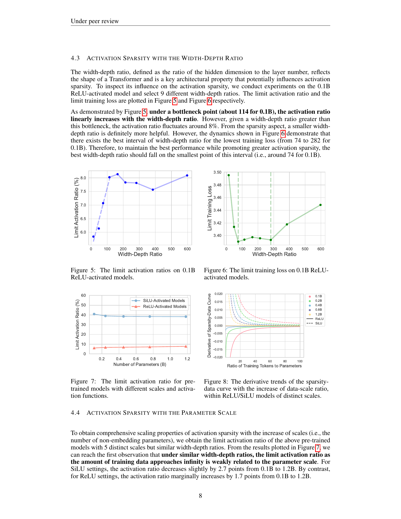
| 0.1B ReLU | 0.1B SiLU | 0.2B ReLU | 0.2B SiLU | 0.4B ReLU | 0.4B SiLU | 0.8B ReLU | 0.8B SiLU | 1.2B ReLU | 1.2B SiLU | ||
|---|---|---|---|---|---|---|---|---|---|---|---|
| C.R. | dense | 49.6 | 49.5 | 52.0 | 52.2 | 54.7 | 55.8 | 56.8 | 57.6 | 60.0 | 59.6 |
| PPL-1% | 49.1 | 49.9 | 51.7 | 52.4 | 54.6 | 55.8 | 55.9 | 57.6 | 59.6 | 59.6 | |
| PPL-5% | 49.2 | 49.0 | 51.7 | 52.0 | 54.3 | 55.1 | 56.3 | 57.1 | 59.3 | 58.8 | |
| PPL-10% | 49.4 | 48.7 | 51.6 | 51.9 | 54.9 | 55.2 | 55.6 | 56.4 | 59.3 | 59.3 | |
| R.C. | dense | 28.2 | 27.7 | 40.7 | 40.2 | 44.0 | 41.8 | 44.8 | 43.3 | 53.2 | 54.8 |
| PPL-1% | 28.4 | 28.0 | 39.7 | 39.6 | 42.9 | 40.9 | 43.2 | 44.3 | 53.3 | 55.4 | |
| PPL-5% | 26.9 | 26.5 | 38.6 | 36.8 | 40.8 | 38.2 | 42.2 | 40.7 | 53.3 | 52.6 | |
| PPL-10% | 26.2 | 24.8 | 38.6 | 34.4 | 39.9 | 35.3 | 40.3 | 38.8 | 52.9 | 51.1 |
🔼 This table presents the average performance scores (in percentages) achieved on two distinct task groups: commonsense reasoning (C.R.) and reading comprehension (R.C.). The results are broken down based on different model configurations, each characterized by varying p% values. The ‘dense’ setting (p=0) represents the benchmark with the most accurate predictions because all neuron outputs are utilized. The other rows show performance and sparsity ratio trade-off at different tolerance levels (percentage of PPL rise).
read the caption
Table 1: The average evaluation scores (%) on two task groups, where C.R. refers to commonsense reasoning and R.C. refers to reading comprehension. The second column represents settings with different p%percent𝑝p\%italic_p % values, with “dense” indicating the most accurate case where p=0𝑝0p=0italic_p = 0.
In-depth insights#
Sparsity Scaling Laws#
The research explores sparsity scaling laws in large language models (LLMs), revealing crucial insights into the relationship between activation sparsity and key factors like training data and model architecture. ReLU activation functions demonstrate superior efficiency in enhancing sparsity compared to SiLU, exhibiting a convergent decreasing relationship with training data. Conversely, SiLU shows a convergent increasing trend. Activation sparsity increases linearly with the width-depth ratio, up to a certain point, highlighting the potential benefits of deeper architectures. Interestingly, the limit of activation sparsity shows weak correlation with the parameter scale, indicating that activation patterns remain consistent across various model sizes, although smaller models achieve convergence faster. These findings offer valuable guidance for designing more efficient and interpretable LLMs by leveraging the potential of greater activation sparsity.
PPL-p% Sparsity Metric#
The research introduces a novel metric, PPL-p% sparsity, to more effectively measure activation sparsity in large language models (LLMs). Unlike previous methods that rely on arbitrary thresholds, this metric directly incorporates model performance (perplexity or PPL), making it performance-aware. It identifies weakly-contributed neurons by adaptively determining layer-wise thresholds, ensuring that the increased perplexity resulting from their inactivation stays within a specified range (p%). This approach offers several advantages: versatility across various model architectures and activation functions, performance-awareness, and precise recognition of weakly-contributed neurons, ultimately providing a more reliable and insightful measure of activation sparsity for LLMs.
Activation Function Effects#
The research reveals a surprising contrast in the behavior of ReLU and SiLU activation functions regarding activation sparsity. While both achieve comparable performance, they exhibit opposite training-time sparsity trends. ReLU-activated LLMs demonstrate a convergent decreasing logspace power-law, becoming increasingly sparse with more training data. Conversely, SiLU-activated models show a convergent increasing power-law, indicating reduced sparsity with increased training. This suggests ReLU is more efficient at leveraging training data for improved activation sparsity. The study also shows that ReLU consistently outperforms SiLU in terms of achieving higher sparsity at comparable performance levels.
Width-Depth Ratio Impact#
The research explores how the width-depth ratio in Transformer-based LLMs significantly impacts activation sparsity. A linear increase in activation ratio is observed with increasing width-depth ratio, up to a specific bottleneck point. Beyond this point, the activation ratio stabilizes, suggesting diminishing returns. This indicates that deeper architectures may be advantageous for achieving higher sparsity at a fixed parameter scale, but there’s an optimal width-depth ratio to consider to avoid performance degradation. The study also reveals a surprising finding that the limit value of activation sparsity at high training data levels is only weakly dependent on the parameter scale.
Future Research#
The paper does not contain a heading explicitly titled ‘Future Research’. Therefore, a summary cannot be provided. However, the conclusion section hints at promising avenues for future work. Investigating the correlation between activation sparsity and neuron specialization is highlighted as a crucial area needing further exploration. This would provide valuable insights into the dynamics of model training and potentially lead to better methods for controlling and promoting activation sparsity. Additionally, extending the research to even larger LLMs with more parameters and evaluating the effects on sparsity patterns is suggested. Finally, a more in-depth analysis of the impact of dataset distribution on sparsity is recommended. This would help to refine the scaling laws and make them more widely applicable and robust across varied datasets.
More visual insights#
More on figures

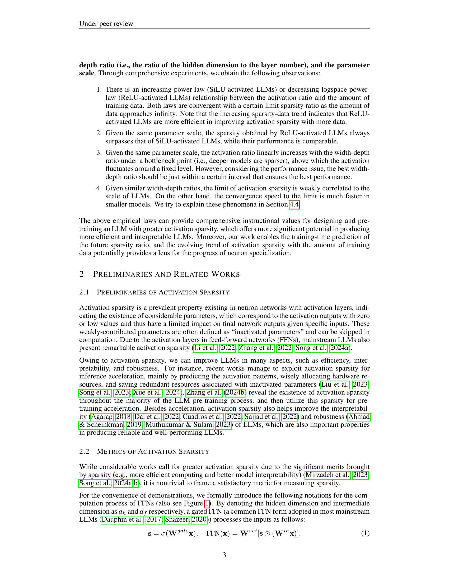
🔼 This figure illustrates the Pareto curves that show the trade-off between activation sparsity and model perplexity (PPL) for different models. The 0.1B parameter MoE (Mixture-of-Experts) model is shown with varying numbers of experts (16, 30, and 60), while the vanilla 0.1B parameter decoder-only Transformer serves as a baseline for comparison. The x-axis represents the activation ratio (1-sparsity ratio), indicating the proportion of activated neurons. The y-axis represents the perplexity, a measure of the model’s prediction accuracy. Lower perplexity indicates better performance, while a higher activation ratio implies lower sparsity. The curves reveal the performance-sparsity trade-off, demonstrating that increasing activation sparsity often comes at the cost of higher perplexity (reduced performance). The comparison highlights the performance-sparsity trade-off differences between MoE and vanilla models.
read the caption
Figure 2: The PPL-activation Pareto curve of the 0.1B MoE with different expert numbers versus the 0.1B vanilla decoder-only Transformer.

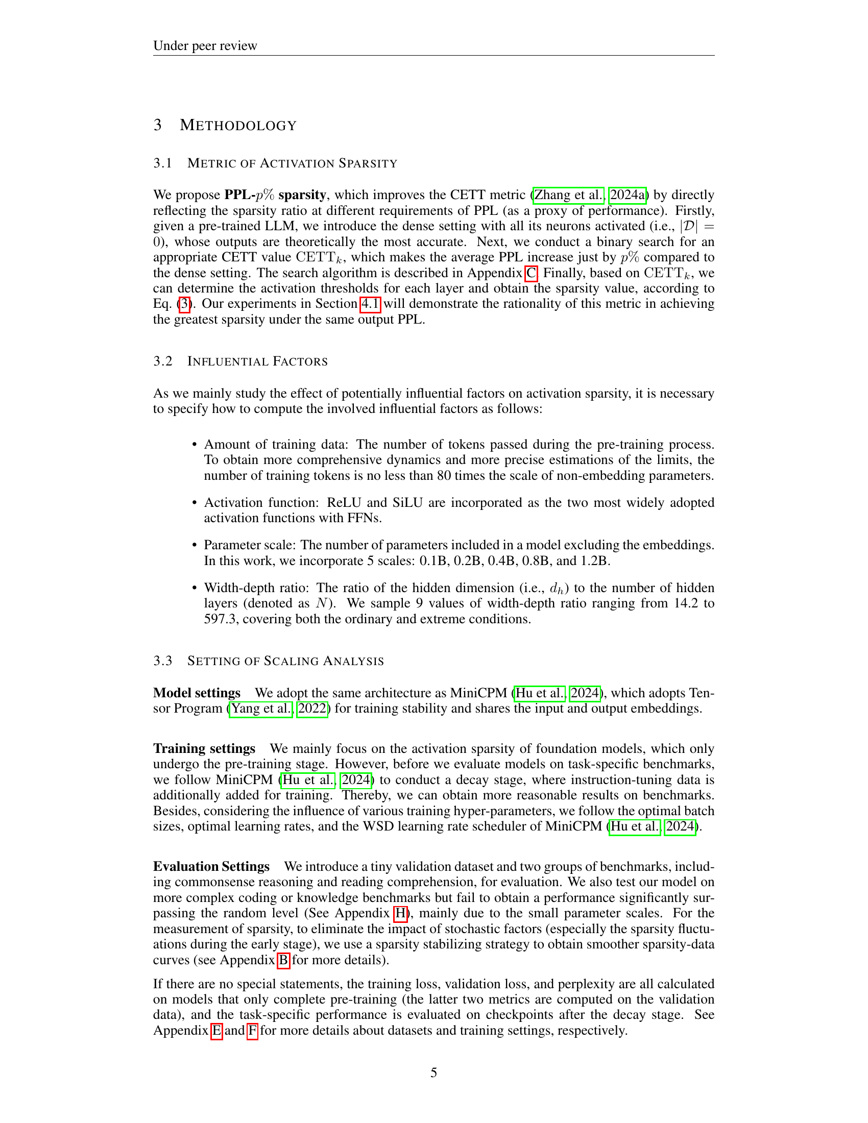
🔼 Figure 3 illustrates the performance-sparsity trade-off for different activation sparsity metrics across various model sizes (0.1B, 0.2B, 0.4B, 0.8B, and 1.2B parameters). It compares the proposed PPL-p% sparsity metric with two baseline methods: a straightforward ReLU-based method (applicable only to ReLU-activated models) and a Top-k sparsity method. The x-axis represents the activation ratio (1 - sparsity ratio), indicating the proportion of activated neurons, and the y-axis shows the perplexity (PPL), a measure of model performance. Each curve represents a different model scale, and each point shows the perplexity given the activation ratio achieved by the corresponding method. This figure demonstrates the effectiveness of the PPL-p% sparsity metric in achieving a better balance between performance and sparsity compared to simpler approaches.
read the caption
Figure 3: The PPL-activation Pareto curve of our PPL-p%percent𝑝p\%italic_p % sparsity versus two baselines within models of different scales. “Straightforward ReLU” is only applicable to ReLU-activated models.

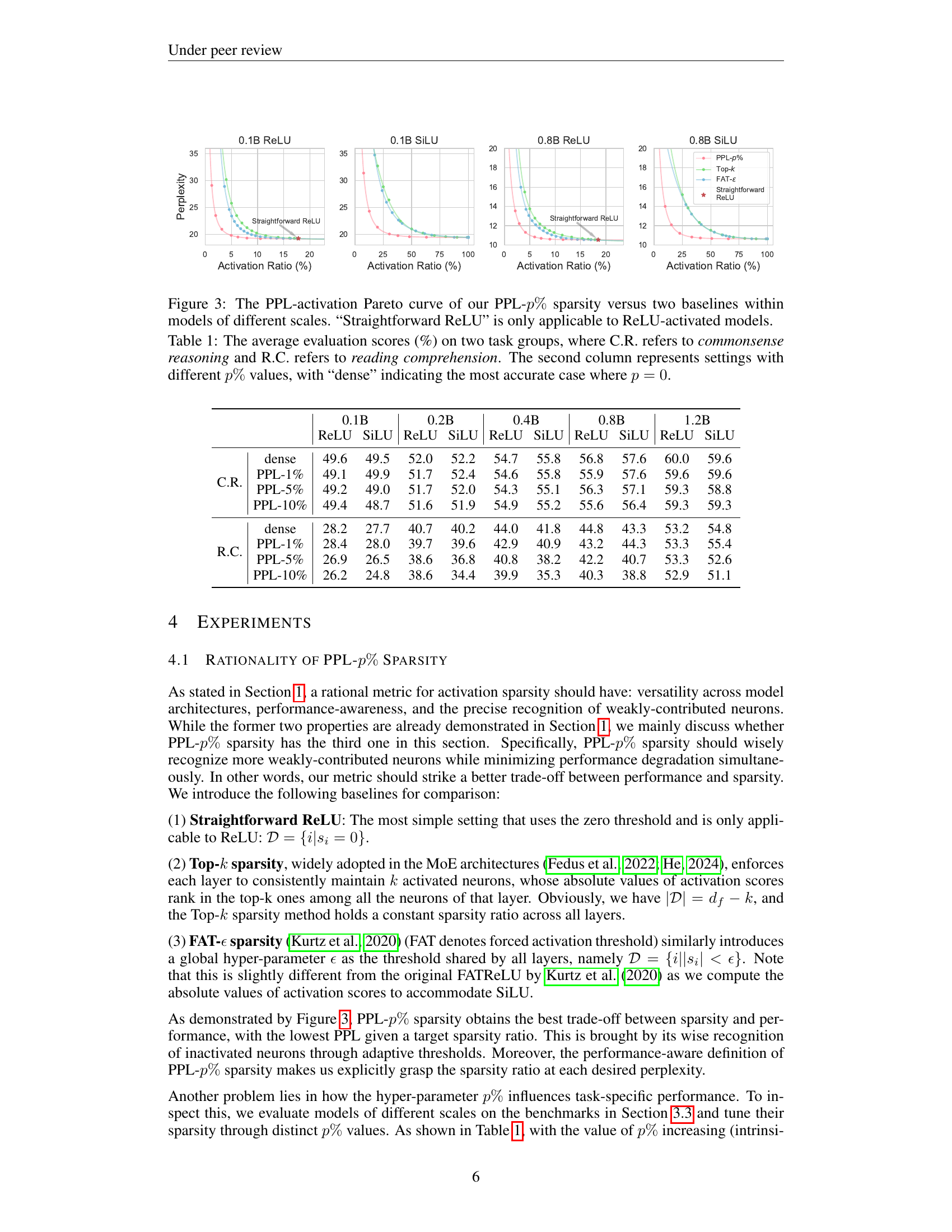
🔼 This figure displays the relationship between activation ratio and the amount of training data for large language models (LLMs) using different activation functions (ReLU and SiLU) and model sizes. The activation ratio, calculated using the PPL-1% sparsity metric, represents the proportion of activated neurons in the model. The x-axis shows the number of tokens (in billions) processed during training, and the y-axis shows the activation ratio. Each line represents a different model size (0.1B, 0.2B, 0.4B, 0.8B, and 1.2B parameters). The brown lines represent curves fitted to the data points. The number of training tokens used was at least 190 times the number of non-embedding parameters in each model. This demonstrates how activation sparsity evolves during training and differs based on activation function and model size.
read the caption
Figure 4: The trend of activation ratios (hereinafter using PPL-1%percent11\%1 % sparsity) of models with different scales and activation functions during the pre-training stage. The fitted curves are plotted in brown. The number of training tokens is no less than 190 times the scale of non-embedding parameters.

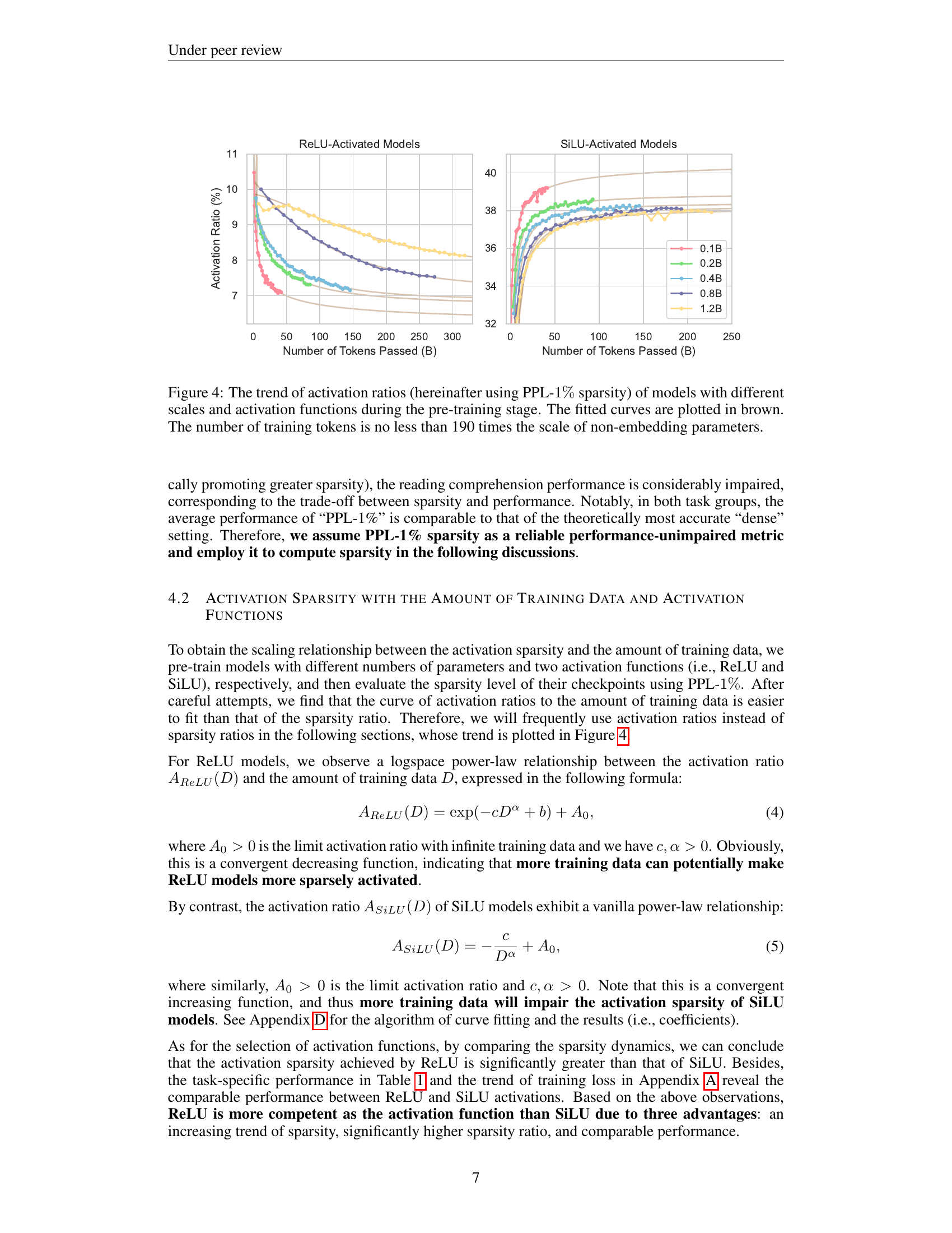
🔼 This figure shows the limit activation ratio for a 0.1B parameter ReLU-activated model across various width-depth ratios. The limit activation ratio represents the sparsity level the model converges to with an infinite amount of training data. The x-axis represents the width-depth ratio (hidden dimension divided by number of layers). The y-axis displays the limit activation ratio. The plot illustrates the relationship between the model’s architecture (width-depth ratio) and its resulting activation sparsity when sufficient training data is used.
read the caption
Figure 5: The limit activation ratios on 0.1B ReLU-activated models.

🔼 This figure shows the relationship between the width-depth ratio and the training loss of a 0.1B parameter ReLU-activated model after extensive training. The width-depth ratio is the ratio of the hidden dimension to the number of layers in the transformer model. The x-axis represents different width-depth ratios, and the y-axis represents the training loss (limit value after extensive training). The graph illustrates that there’s a minimum training loss within a specific range of width-depth ratios, indicating an optimal model architecture for this specific configuration. Outside of this range, the training loss increases, implying that a wider or narrower architecture can negatively impact performance.
read the caption
Figure 6: The limit training loss on 0.1B ReLU-activated models.

🔼 This figure shows the limit of activation sparsity (activation ratio) for pre-trained language models with varying parameter scales and activation functions. The limit represents the activation ratio as the amount of training data approaches infinity. Separate lines are plotted to show the values for models using the ReLU activation function and those using the SiLU activation function. The x-axis shows the parameter scale of the model, and the y-axis displays the limit activation ratio. This helps in understanding the relationship between model scale, activation function choice, and the resulting sparsity.
read the caption
Figure 7: The limit activation ratio for pre-trained models with different scales and activation functions.

🔼 Figure 8 shows how the rate of change in activation sparsity changes as the amount of training data increases relative to the model size (parameter scale). Separate lines are plotted for both ReLU and SiLU activation functions, and different colored lines represent models of varying sizes (0.1B, 0.2B, 0.4B, 0.8B, 1.2B parameters). The figure visualizes the convergence speed towards a limit of sparsity as training data increases. It shows that smaller models reach their sparsity limits faster than larger models.
read the caption
Figure 8: The derivative trends of the sparsity-data curve with the increase of data-scale ratio, within ReLU/SiLU models of distinct scales.

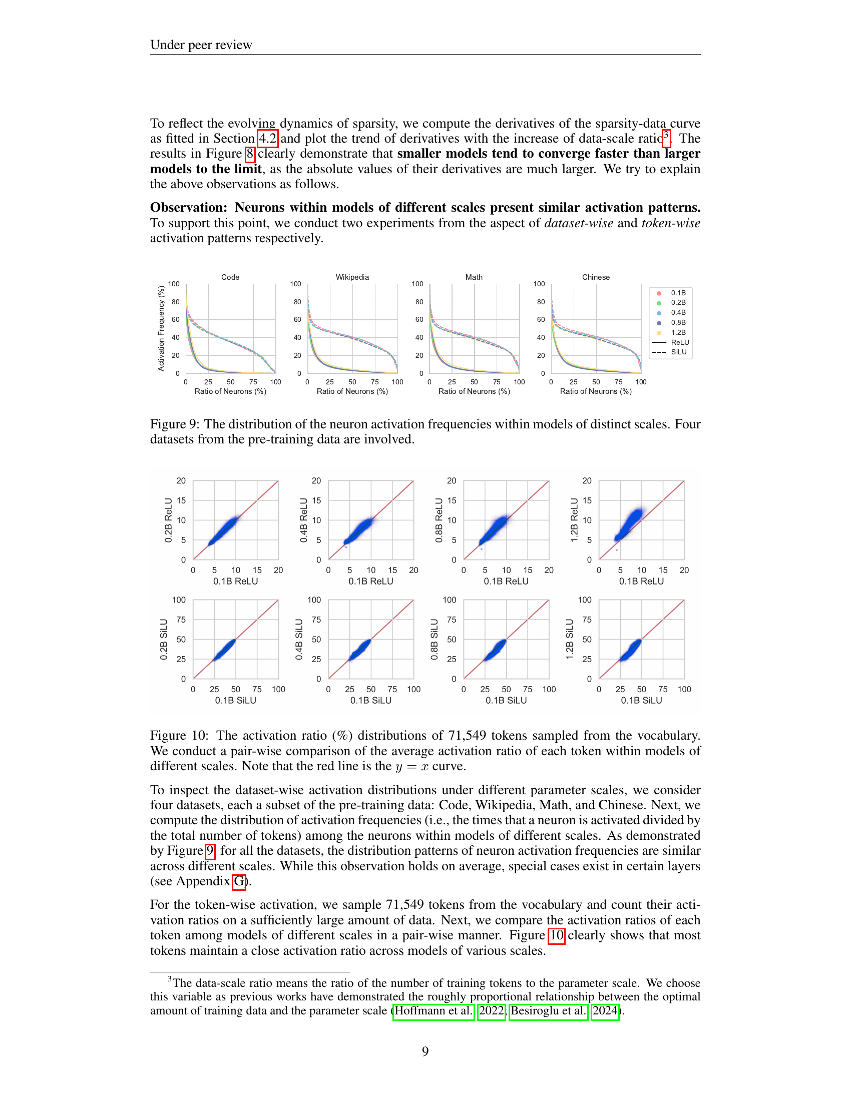
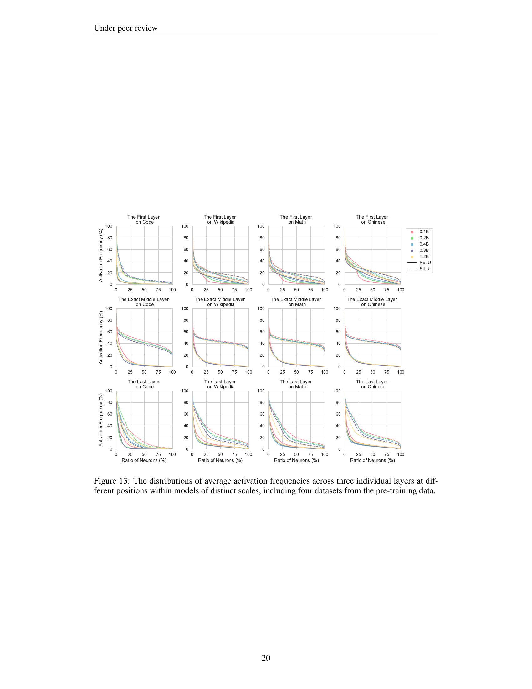
🔼 Figure 9 illustrates the distribution of neuron activation frequencies across models of varying sizes (0.1B, 0.2B, 0.4B, 0.8B, and 1.2B parameters). The analysis focuses on how frequently each neuron is activated during the model’s pre-training phase. To provide context, the data is partitioned into four distinct datasets used in the pre-training process: Code, Wikipedia, Math, and Chinese. This visualization helps to understand whether activation patterns remain consistent across different model scales and datasets, offering insights into the scaling properties of neuron activation behavior.
read the caption
Figure 9: The distribution of the neuron activation frequencies within models of distinct scales. Four datasets from the pre-training data are involved.

🔼 Figure 10 visually examines the consistency of activation patterns across various model scales. It displays the distribution of activation ratios for 71,549 randomly selected tokens from the vocabulary. A pairwise comparison is made showing the average activation ratio of each token across models of different sizes (0.1B, 0.2B, 0.4B, 0.8B, and 1.2B parameters) for both ReLU and SiLU activation functions. The red line represents a perfect correlation (y=x), indicating identical activation ratios across models. Deviations from this line highlight differences in activation behavior across different parameter scales for specific tokens.
read the caption
Figure 10: The activation ratio (%) distributions of 71,549 tokens sampled from the vocabulary. We conduct a pair-wise comparison of the average activation ratio of each token within models of different scales. Note that the red line is the y=x𝑦𝑥y=xitalic_y = italic_x curve.

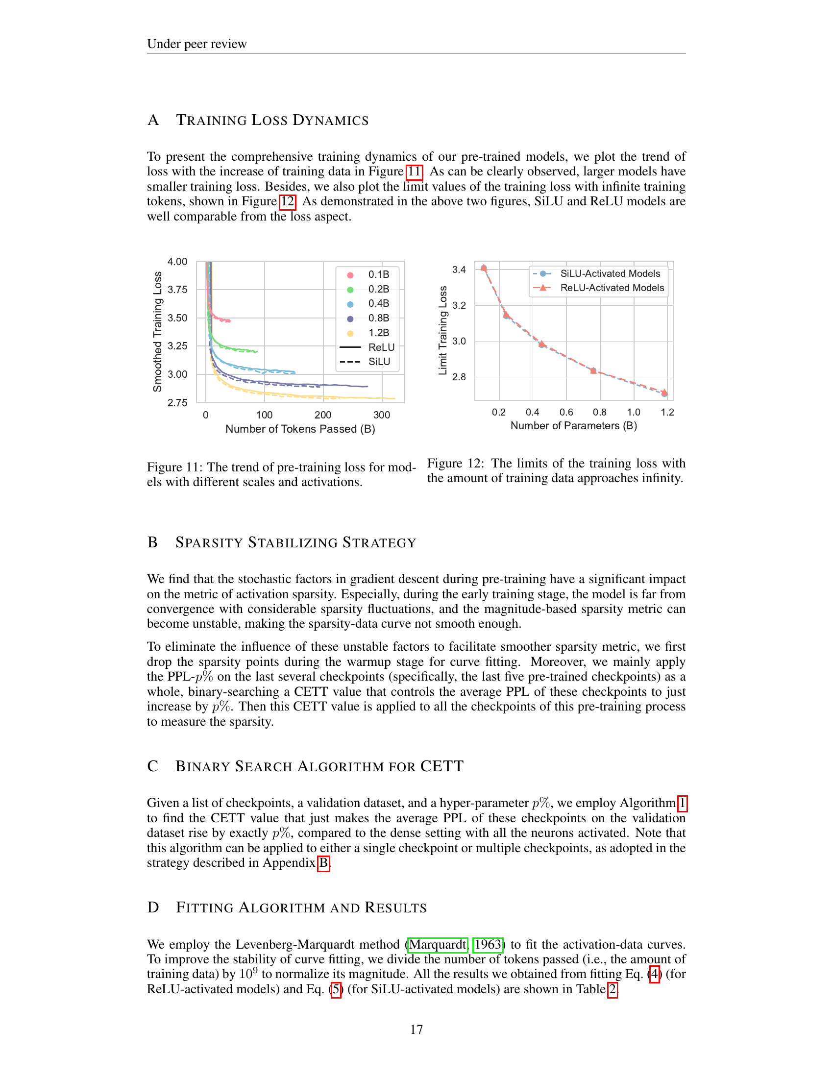
🔼 This figure visualizes the training loss curves for different sized language models during the pre-training phase. The models vary in scale (0.1B, 0.2B, 0.4B, 0.8B, and 1.2B parameters) and use either ReLU or SiLU activation functions. The x-axis represents the number of tokens processed during training, and the y-axis shows the training loss. This allows for a comparison of the training dynamics across various model sizes and activation functions.
read the caption
Figure 11: The trend of pre-training loss for models with different scales and activations.

🔼 This figure shows the convergence points of training loss for different model sizes and activation functions as the amount of training data approaches infinity. It illustrates the minimum achievable training loss for each model configuration, indicating the potential efficiency limits for each.
read the caption
Figure 12: The limits of the training loss with the amount of training data approaches infinity.

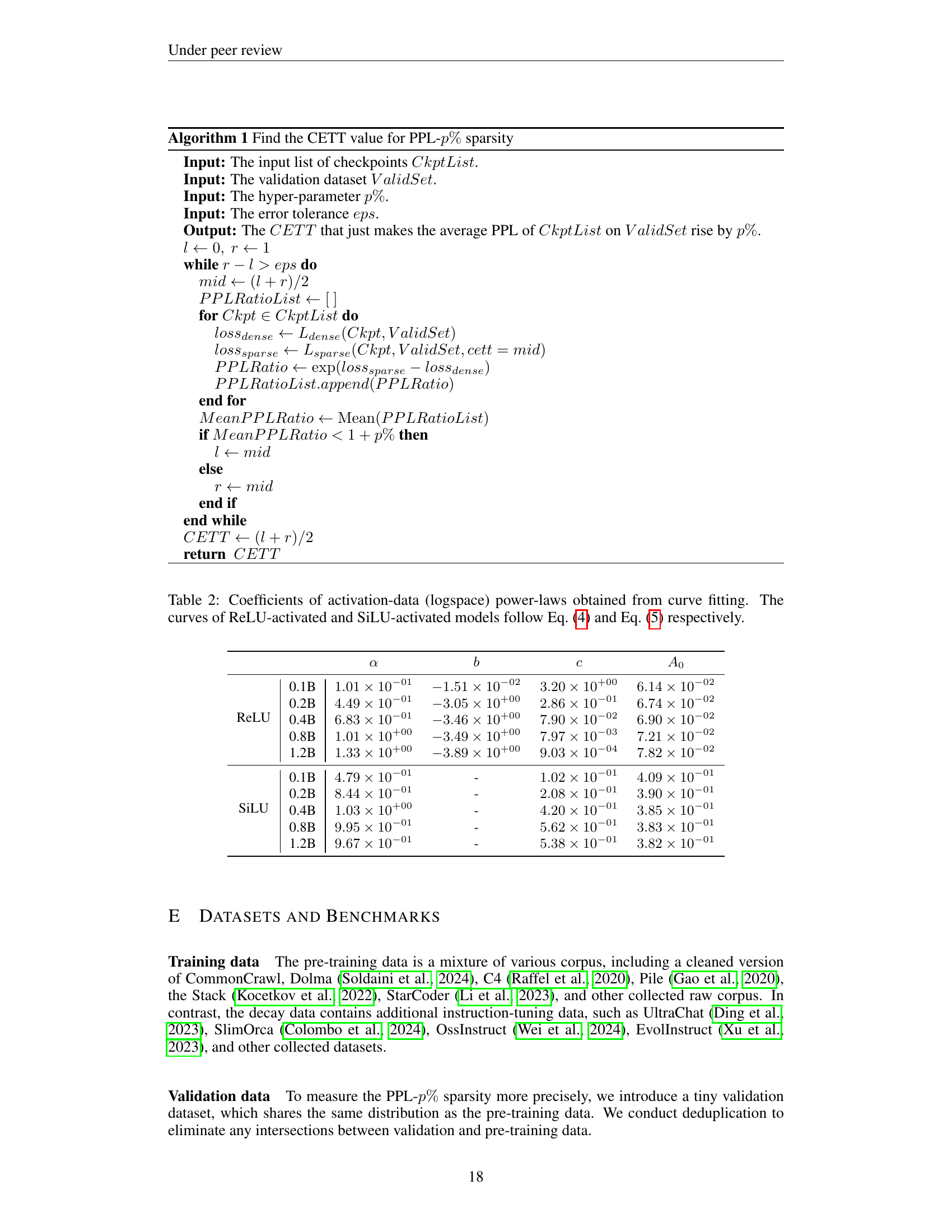
🔼 The algorithm performs a binary search to find an optimal cumulative error of tail truncation (CETT) value. This CETT value, when applied to a list of model checkpoints, results in an increase of the average perplexity (PPL) by a specified percentage (p%). The algorithm iteratively adjusts the CETT value, evaluating the average PPL on a validation dataset for each adjustment. The process continues until the desired PPL increase is achieved within a specified error tolerance. The final CETT value represents the sparsity level that balances model performance and sparsity.
read the caption
Algorithm 1 Find the CETT value for PPL-p%percent𝑝p\%italic_p % sparsity
More on tables
| α | b | c | A₀ | |
|---|---|---|---|---|
| ReLU | 0.1B | $1.01 \times 10^{-01}$ | $-1.51 \times 10^{-02}$ | $3.20 \times 10^{+00}$ |
| 0.2B | $4.49 \times 10^{-01}$ | $-3.05 \times 10^{+00}$ | $2.86 \times 10^{-01}$ | |
| 0.4B | $6.83 \times 10^{-01}$ | $-3.46 \times 10^{+00}$ | $7.90 \times 10^{-02}$ | |
| 0.8B | $1.01 \times 10^{+00}$ | $-3.49 \times 10^{+00}$ | $7.97 \times 10^{-03}$ | |
| 1.2B | $1.33 \times 10^{+00}$ | $-3.89 \times 10^{+00}$ | $9.03 \times 10^{-04}$ | |
| SiLU | 0.1B | $4.79 \times 10^{-01}$ | - | $4.09 \times 10^{-01}$ |
| 0.2B | $8.44 \times 10^{-01}$ | - | $3.90 \times 10^{-01}$ | |
| 0.4B | $1.03 \times 10^{+00}$ | - | $3.85 \times 10^{-01}$ | |
| 0.8B | $9.95 \times 10^{-01}$ | - | $3.83 \times 10^{-01}$ | |
| 1.2B | $9.67 \times 10^{-01}$ | - | $3.82 \times 10^{-01}$ |
🔼 This table presents the coefficients derived from fitting power-law curves to the relationship between activation sparsity and the amount of training data for both ReLU and SiLU activation functions in large language models. The fitting is done separately for different model sizes (parameter scales) and activation functions. The ’logspace’ nature of the power-law is highlighted for ReLU, meaning that sparsity changes logarithmically with training data; whereas it is a standard power law for SiLU. The coefficients a, b, c, and A0 are presented for each model size and activation type, allowing for reconstruction of the sparsity curve using equations (4) and (5).
read the caption
Table 2: Coefficients of activation-data (logspace) power-laws obtained from curve fitting. The curves of ReLU-activated and SiLU-activated models follow Eq. (4) and Eq. (5) respectively.
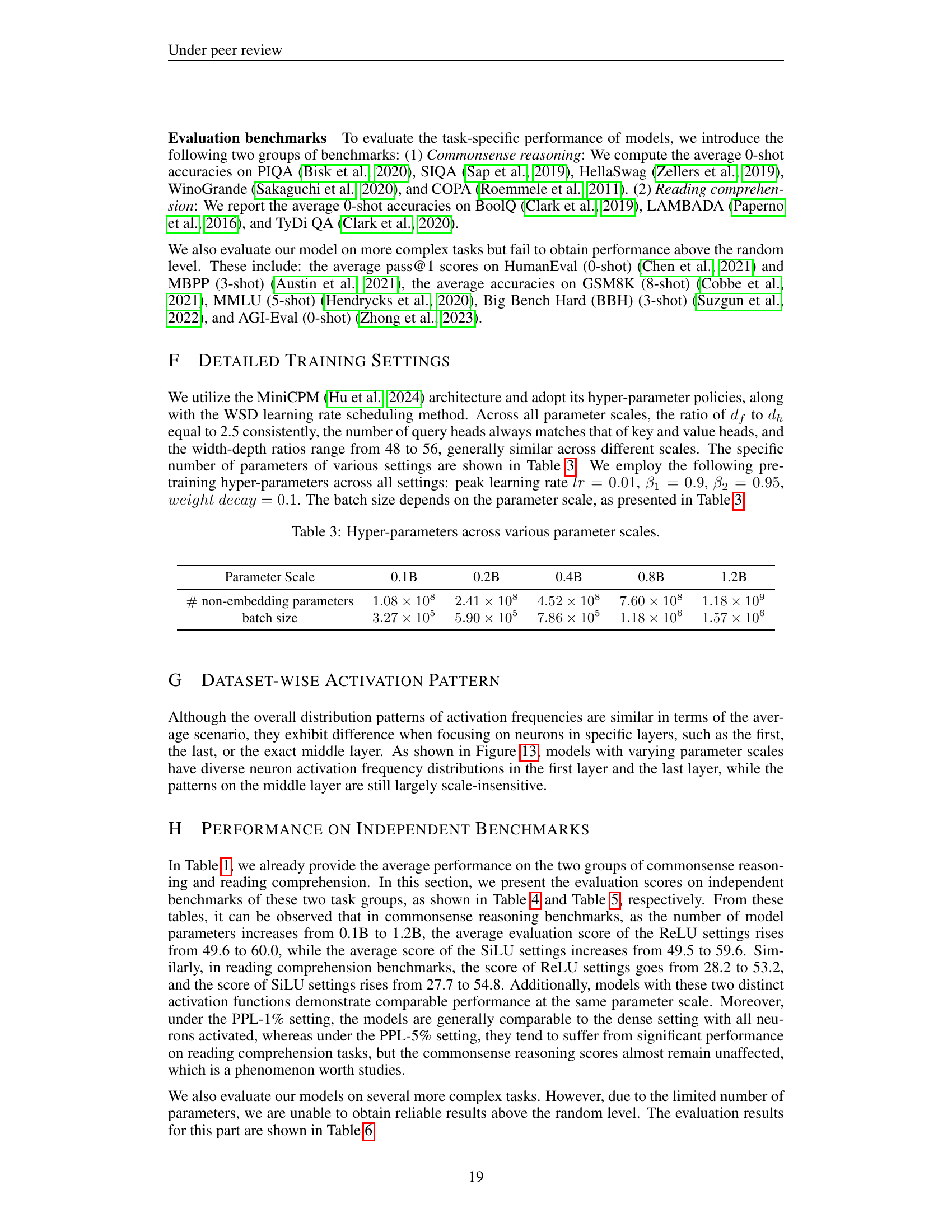
| Parameter Scale | 0.1B | 0.2B | 0.4B | 0.8B | 1.2B |
|---|---|---|---|---|---|
| # non-embedding parameters | 1.08e+08 | 2.41e+08 | 4.52e+08 | 7.60e+08 | 1.18e+09 |
| batch size | 3.27e+05 | 5.90e+05 | 7.86e+05 | 1.18e+06 | 1.57e+06 |
🔼 This table shows the hyper-parameter settings used for training the language models with different parameter scales (0.1B, 0.2B, 0.4B, 0.8B, and 1.2B). It details the number of non-embedding parameters, and the batch size used during training for each model size. The values reflect the settings chosen to ensure optimal training stability and performance for the different model scales.
read the caption
Table 3: Hyper-parameters across various parameter scales.
| Model Size | Activation | Variant | PIQA acc | SIQA acc | HellaSwag acc | WinoGrande acc | COPA acc | Avg. acc | |
|---|---|---|---|---|---|---|---|---|---|
| 0.1B | ReLU | dense | 62.8 | 37.8 | 30.5 | 53.0 | 64.0 | 49.6 | |
| PPL-1% | 62.7 | 37.4 | 30.5 | 52.6 | 62.0 | 49.1 | |||
| PPL-5% | 63.1 | 37.6 | 30.3 | 51.1 | 64.0 | 49.2 | |||
| PPL-10% | 63.0 | 38.0 | 30.5 | 51.5 | 64.0 | 49.4 | |||
| SiLU | dense | 64.3 | 37.6 | 30.9 | 52.8 | 62.0 | 49.5 | ||
| PPL-1% | 64.3 | 37.5 | 30.7 | 53.0 | 64.0 | 49.9 | |||
| PPL-5% | 63.5 | 38.4 | 30.5 | 51.5 | 61.0 | 49.0 | |||
| PPL-10% | 63.8 | 38.1 | 30.4 | 51.3 | 60.0 | 48.7 | |||
| 0.2B | ReLU | dense | 66.3 | 38.3 | 37.1 | 53.1 | 65.0 | 52.0 | |
| PPL-1% | 66.3 | 38.1 | 37.2 | 52.7 | 64.0 | 51.7 | |||
| PPL-5% | 66.2 | 38.1 | 37.1 | 52.2 | 65.0 | 51.7 | |||
| PPL-10% | 66.0 | 37.9 | 37.0 | 51.9 | 65.0 | 51.6 | |||
| SiLU | dense | 67.6 | 39.0 | 37.8 | 51.8 | 65.0 | 52.2 | ||
| PPL-1% | 68.2 | 39.2 | 37.7 | 52.0 | 65.0 | 52.4 | |||
| PPL-5% | 67.4 | 38.2 | 37.7 | 51.8 | 65.0 | 52.0 | |||
| PPL-10% | 66.8 | 38.8 | 37.9 | 52.1 | 64.0 | 51.9 | |||
| 0.4B | ReLU | dense | 68.8 | 39.9 | 42.7 | 51.9 | 70.0 | 54.7 | |
| PPL-1% | 68.8 | 39.7 | 42.9 | 51.8 | 70.0 | 54.6 | |||
| PPL-5% | 68.3 | 39.9 | 42.7 | 52.5 | 68.0 | 54.3 | |||
| PPL-10% | 68.1 | 40.4 | 42.6 | 53.2 | 70.0 | 54.9 | |||
| SiLU | dense | 69.0 | 39.6 | 44.5 | 51.9 | 74.0 | 55.8 | ||
| PPL-1% | 68.7 | 39.4 | 44.6 | 52.2 | 74.0 | 55.8 | |||
| PPL-5% | 68.9 | 39.4 | 44.6 | 51.5 | 71.0 | 55.1 | |||
| PPL-10% | 68.7 | 39.3 | 44.9 | 51.0 | 72.0 | 55.2 | |||
| 0.8B | ReLU | dense | 70.1 | 41.8 | 50.4 | 53.6 | 68.0 | 56.8 | |
| PPL-1% | 69.8 | 41.8 | 50.2 | 52.8 | 65.0 | 55.9 | |||
| PPL-5% | 69.9 | 41.8 | 49.7 | 52.3 | 68.0 | 56.3 | |||
| PPL-10% | 69.6 | 41.8 | 50.0 | 51.8 | 65.0 | 55.6 | |||
| SiLU | dense | 70.4 | 40.9 | 50.6 | 54.0 | 72.0 | 57.6 | ||
| PPL-1% | 70.3 | 41.4 | 50.6 | 53.9 | 72.0 | 57.6 | |||
| PPL-5% | 69.9 | 41.3 | 51.0 | 54.1 | 69.0 | 57.1 | |||
| PPL-10% | 69.5 | 40.7 | 50.6 | 53.2 | 68.0 | 56.4 | |||
| 1.2B | ReLU | dense | 71.6 | 44.1 | 57.7 | 56.4 | 70.0 | 60.0 | |
| PPL-1% | 71.1 | 44.7 | 58.0 | 55.3 | 69.0 | 59.6 | |||
| PPL-5% | 70.8 | 43.9 | 57.8 | 54.9 | 69.0 | 59.3 | |||
| PPL-10% | 70.2 | 43.6 | 57.1 | 53.7 | 72.0 | 59.3 | |||
| SiLU | dense | 71.8 | 41.2 | 57.8 | 56.1 | 71.0 | 59.6 | ||
| PPL-1% | 71.8 | 40.9 | 57.8 | 57.3 | 70.0 | 59.6 | |||
| PPL-5% | 71.8 | 41.3 | 57.9 | 55.9 | 67.0 | 58.8 | |||
| PPL-10% | 71.6 | 41.3 | 58.1 | 55.5 | 70.0 | 59.3 |
🔼 This table presents the performance of various LLMs on commonsense reasoning benchmarks. Different model sizes (0.1B, 0.2B, 0.4B, 0.8B, 1.2B parameters) and activation functions (ReLU and SiLU) are evaluated. For each model configuration, the ‘dense’ setting represents the full model performance, while PPL-1%, PPL-5%, and PPL-10% represent performance at different levels of activation sparsity. The results are shown as accuracy scores (%) for five specific commonsense reasoning datasets (PIQA, SIQA, HellaSwag, WinoGrande, and COPA), with a final average score across these datasets also included. This allows comparison of model accuracy across different sparsity levels and configurations.
read the caption
Table 4: Evaluation scores (%) on commonsense reasoning benchmarks.
| Parameter | Activation | Method | BoolQ acc | LAMBADA acc | TyDiQA F1 | TyDiQA acc | Avg. |
|---|---|---|---|---|---|---|---|
| 0.1B | ReLU | dense | 60.8 | 30.1 | 17.9 | 4.1 | 28.2 |
| PPL-1% | 60.6 | 28.5 | 19.9 | 4.5 | 28.4 | ||
| PPL-5% | 60.6 | 25.6 | 17.9 | 3.4 | 26.9 | ||
| PPL-10% | 60.1 | 24.6 | 16.4 | 3.9 | 26.2 | ||
| SiLU | dense | 56.5 | 31.4 | 18.5 | 4.5 | 27.7 | |
| PPL-1% | 56.2 | 31.1 | 19.1 | 5.5 | 28.0 | ||
| PPL-5% | 53.6 | 28.9 | 18.0 | 5.5 | 26.5 | ||
| PPL-10% | 51.9 | 25.7 | 16.6 | 5.0 | 24.8 | ||
| 0.2B | ReLU | dense | 56.3 | 38.4 | 38.0 | 30.0 | 40.7 |
| PPL-1% | 56.2 | 35.8 | 36.8 | 30.0 | 39.7 | ||
| PPL-5% | 56.4 | 33.0 | 36.3 | 28.6 | 38.6 | ||
| PPL-10% | 55.9 | 30.8 | 37.4 | 30.2 | 38.6 | ||
| SiLU | dense | 57.5 | 38.7 | 36.3 | 28.2 | 40.2 | |
| PPL-1% | 57.5 | 38.3 | 35.3 | 27.5 | 39.6 | ||
| PPL-5% | 55.2 | 36.0 | 31.6 | 24.3 | 36.8 | ||
| PPL-10% | 54.5 | 34.0 | 28.1 | 20.9 | 34.4 | ||
| 0.4B | ReLU | dense | 61.7 | 42.9 | 43.6 | 28.0 | 44.0 |
| PPL-1% | 61.6 | 41.3 | 42.1 | 26.6 | 42.9 | ||
| PPL-5% | 60.8 | 39.1 | 39.9 | 23.4 | 40.8 | ||
| PPL-10% | 60.2 | 37.8 | 39.2 | 22.5 | 39.9 | ||
| SiLU | dense | 57.6 | 43.0 | 41.1 | 25.4 | 41.8 | |
| PPL-1% | 56.6 | 43.1 | 40.5 | 23.4 | 40.9 | ||
| PPL-5% | 55.2 | 39.2 | 38.1 | 20.4 | 38.2 | ||
| PPL-10% | 52.7 | 35.9 | 35.0 | 17.7 | 35.3 | ||
| 0.8B | ReLU | dense | 62.1 | 47.3 | 42.6 | 27.3 | 44.8 |
| PPL-1% | 61.7 | 45.7 | 41.0 | 24.6 | 43.2 | ||
| PPL-5% | 60.9 | 43.8 | 40.0 | 24.1 | 42.2 | ||
| PPL-10% | 59.8 | 42.5 | 37.8 | 21.1 | 40.3 | ||
| SiLU | dense | 63.1 | 46.9 | 41.0 | 22.1 | 43.3 | |
| PPL-1% | 63.1 | 46.0 | 43.3 | 24.8 | 44.3 | ||
| PPL-5% | 62.5 | 44.7 | 37.5 | 18.2 | 40.7 | ||
| PPL-10% | 62.7 | 43.0 | 34.6 | 15.0 | 38.8 | ||
| 1.2B | ReLU | dense | 63.3 | 52.5 | 54.3 | 42.5 | 53.2 |
| PPL-1% | 63.4 | 52.2 | 55.0 | 42.7 | 53.3 | ||
| PPL-5% | 62.1 | 49.5 | 56.3 | 45.2 | 53.3 | ||
| PPL-10% | 62.6 | 47.7 | 56.8 | 44.5 | 52.9 | ||
| SiLU | dense | 63.2 | 53.4 | 55.2 | 47.3 | 54.8 | |
| PPL-1% | 63.7 | 54.2 | 56.1 | 47.5 | 55.4 | ||
| PPL-5% | 62.2 | 51.2 | 53.1 | 43.9 | 52.6 | ||
| PPL-10% | 60.2 | 47.5 | 53.1 | 43.4 | 51.1 |
🔼 This table presents the evaluation results of different models on various reading comprehension benchmarks. The benchmarks include BoolQ, LAMBADA, TyDiQA-F1, and TyDiQA-Accuracy. The results are shown as percentage scores for each model, broken down by model size (0.1B, 0.2B, 0.4B, 0.8B, 1.2B parameters) and activation function (ReLU, SiLU), and further categorized by different sparsity levels (dense, PPL-1%, PPL-5%, and PPL-10%). The ‘Avg’ column provides an average score across the four benchmarks for each model and sparsity level.
read the caption
Table 5: Evaluation scores (%) on reading comprehension benchmarks.
| Model Size | Activation | Method | AGIEval acc | HumanEval pass@1 | MBPP pass@1 | GSM8K acc | MMLU acc | BBH acc | Avg. |
|---|---|---|---|---|---|---|---|---|---|
| 0.1B | ReLU | dense | 23.4 | 0.6 | 0.3 | 1.8 | 26.3 | 29.3 | 13.6 |
| PPL-1% | 23.3 | 0.6 | 0.3 | 1.7 | 26.5 | 29.5 | 13.7 | ||
| PPL-5% | 23.5 | 0.6 | 0.1 | 1.9 | 26.3 | 28.7 | 13.5 | ||
| PPL-10% | 23.4 | 0.0 | 0.2 | 1.4 | 26.4 | 29.7 | 13.5 | ||
| SiLU | dense | 23.6 | 0.6 | 0.8 | 1.6 | 26.1 | 29.2 | 13.7 | |
| PPL-1% | 23.5 | 0.6 | 0.4 | 2.1 | 25.6 | 28.5 | 13.4 | ||
| PPL-5% | 23.6 | 0.6 | 0.3 | 1.4 | 25.8 | 30.6 | 13.7 | ||
| PPL-10% | 23.0 | 1.2 | 0.4 | 1.4 | 25.8 | 29.0 | 13.5 | ||
| 0.2B | ReLU | dense | 23.2 | 2.4 | 1.5 | 1.6 | 27.2 | 28.8 | 14.1 |
| PPL-1% | 22.8 | 2.4 | 1.2 | 2.1 | 26.9 | 30.3 | 14.3 | ||
| PPL-5% | 22.7 | 2.4 | 1.0 | 1.6 | 27.1 | 29.7 | 14.1 | ||
| PPL-10% | 23.0 | 2.4 | 1.2 | 2.1 | 26.4 | 30.1 | 14.2 | ||
| SiLU | dense | 24.2 | 4.3 | 1.0 | 2.2 | 25.7 | 29.6 | 14.5 | |
| PPL-1% | 24.2 | 4.3 | 1.8 | 2.0 | 25.2 | 29.1 | 14.4 | ||
| PPL-5% | 23.9 | 5.5 | 1.6 | 1.4 | 25.0 | 29.0 | 14.4 | ||
| PPL-10% | 23.2 | 3.0 | 0.5 | 2.4 | 24.2 | 28.4 | 13.6 | ||
| 0.4B | ReLU | dense | 24.6 | 6.7 | 2.3 | 2.1 | 26.1 | 30.3 | 15.3 |
| PPL-1% | 24.3 | 7.9 | 3.1 | 1.9 | 26.2 | 30.1 | 15.6 | ||
| PPL-5% | 24.6 | 7.9 | 2.9 | 2.2 | 26.6 | 30.2 | 15.7 | ||
| PPL-10% | 25.0 | 7.3 | 2.7 | 2.4 | 26.5 | 29.8 | 15.6 | ||
| SiLU | dense | 24.4 | 5.5 | 3.2 | 2.6 | 24.9 | 30.6 | 15.2 | |
| PPL-1% | 24.6 | 5.5 | 3.7 | 3.3 | 25.8 | 29.4 | 15.4 | ||
| PPL-5% | 24.5 | 6.1 | 2.9 | 3.8 | 25.3 | 29.6 | 15.4 | ||
| PPL-10% | 24.2 | 4.9 | 2.3 | 2.7 | 24.6 | 30.1 | 14.8 | ||
| 0.8B | ReLU | dense | 25.4 | 9.2 | 5.3 | 4.2 | 26.3 | 30.1 | 16.7 |
| PPL-1% | 25.7 | 9.2 | 5.8 | 4.5 | 26.3 | 30.0 | 16.9 | ||
| PPL-5% | 25.3 | 8.5 | 5.4 | 4.5 | 26.5 | 29.8 | 16.7 | ||
| PPL-10% | 25.8 | 8.5 | 5.0 | 4.0 | 26.4 | 29.2 | 16.5 | ||
| SiLU | dense | 25.4 | 9.2 | 4.7 | 4.1 | 24.7 | 28.9 | 16.1 | |
| PPL-1% | 25.1 | 7.9 | 4.6 | 4.0 | 24.8 | 29.7 | 16.0 | ||
| PPL-5% | 25.1 | 7.3 | 3.8 | 3.6 | 24.5 | 29.4 | 15.6 | ||
| PPL-10% | 24.8 | 7.3 | 3.9 | 3.0 | 24.2 | 28.8 | 15.3 | ||
| 1.2B | ReLU | dense | 26.6 | 7.3 | 6.2 | 6.4 | 33.4 | 29.9 | 18.3 |
| PPL-1% | 26.5 | 9.8 | 7.8 | 7.7 | 33.9 | 30.3 | 19.3 | ||
| PPL-5% | 25.8 | 7.9 | 7.4 | 6.3 | 34.3 | 30.2 | 18.6 | ||
| PPL-10% | 25.9 | 7.3 | 6.6 | 5.9 | 34.0 | 30.6 | 18.4 | ||
| SiLU | dense | 26.2 | 9.8 | 9.0 | 5.2 | 32.6 | 30.9 | 18.9 | |
| PPL-1% | 27.0 | 11.0 | 8.9 | 5.8 | 32.2 | 30.4 | 19.2 | ||
| PPL-5% | 25.7 | 7.9 | 8.5 | 5.1 | 31.0 | 30.0 | 18.0 | ||
| PPL-10% | 25.6 | 9.2 | 6.9 | 4.0 | 30.7 | 30.1 | 17.8 |
🔼 Table 6 presents the performance of models with different parameter scales and sparsity levels on six complex benchmarks: AGIEval, HumanEval, MBPP, GSM8K, MMLU, and BBH. It shows the accuracy (acc) or pass@1 rate for each benchmark and model configuration, offering a comprehensive comparison across various tasks and settings, allowing for assessment of model capabilities and the impact of different sparsity techniques.
read the caption
Table 6: Evaluation scores (%) on other more complex benchmarks.
Full paper#
