↗ arXiv ↗ Hugging Face ↗ Papers with Code
TL;DR#
This research investigates whether scaling video generation models improves their understanding of physical laws. Current models struggle to accurately predict the behavior of objects in scenarios beyond those seen during training (out-of-distribution generalization). This is a critical issue because understanding fundamental physical laws is a key requirement for building general-purpose simulators and world models.
The researchers created a 2D physics simulation to generate training data, enabling a quantitative evaluation of video generation model accuracy. They tested in-distribution, out-of-distribution, and combinatorial generalization scenarios. Results show that while scaling improves performance in-distribution and for combinatorial generalization, it fails to significantly improve out-of-distribution scenarios. Furthermore, analysis reveals that the models don’t learn general physical rules but instead prioritize visual features like color over physics-based properties, suggesting the need for new approaches beyond simply scaling model and data size.
Key Takeaways#
Why does it matter?#
This paper is crucial because it challenges the common assumption that simply scaling up video generation models will automatically lead to an understanding of fundamental physical laws. It provides a rigorous empirical evaluation framework and reveals the limitations of current models in out-of-distribution generalization, thereby guiding future research towards more robust and physically grounded world models. This is highly relevant given the recent surge of interest in world models for applications in robotics and other AI domains.
Visual Insights#

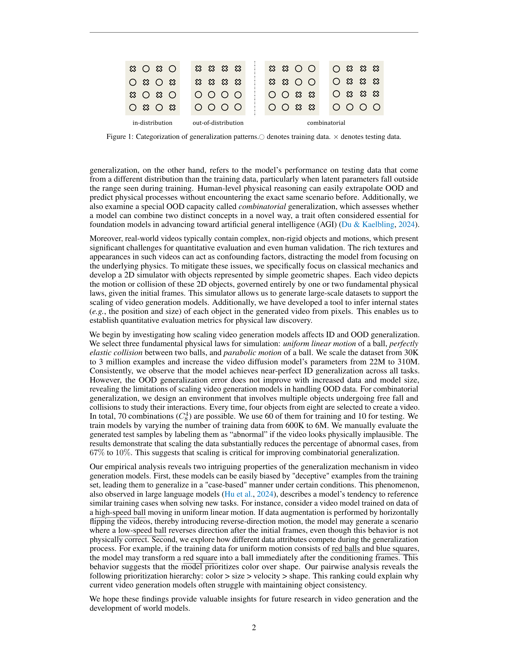
🔼 This figure categorizes generalization patterns in machine learning models by illustrating the relationship between training and testing data. The symbols ○ represent training data points, while × symbols represent test data points. Different panels show in-distribution (ID) generalization where training and testing data come from the same distribution, out-of-distribution (OOD) generalization where testing data comes from a different distribution, and combinatorial generalization where testing data involves novel combinations of concepts observed during training. This visualization aids in understanding how well a model generalizes beyond its training data and in different contexts.
read the caption
Figure 1: Categorization of generalization patterns.○○\ocircle○ denotes training data. ×\times× denotes testing data.
| Model | Layers | Hidden size | Heads | #Param |
|---|---|---|---|---|
| DiT-S | 12 | 384 | 6 | 22.5M |
| DiT-B | 12 | 768 | 12 | 89.5M |
| DiT-L | 24 | 1024 | 16 | 310.0M |
| DiT-XL | 28 | 1152 | 16 | 456.0M |
🔼 This table presents the specifications of four different sizes of Diffusion Transformer (DiT) models used in the experiments. It shows the number of layers, hidden size, number of attention heads, and the total number of parameters for each model size (DiT-S, DiT-B, DiT-L, DiT-XL). These details are crucial for understanding the computational cost and capacity differences between the models.
read the caption
Table 1: Details of DiT model sizes.
In-depth insights#
Physics Law Limits#
The research explores video generation models’ ability to learn and apply fundamental physics laws, focusing on the limitations. The models struggle with out-of-distribution (OOD) generalization, failing to extrapolate learned patterns to unseen scenarios. While in-distribution performance improves with scaling, OOD performance remains poor, indicating that simple scaling isn’t sufficient for true physical understanding. The analysis reveals a ‘case-based’ generalization mechanism, where models prioritize mimicking training examples over abstracting general physical rules. This is evidenced by a hierarchy of attribute prioritization in generalization: color > size > velocity > shape, suggesting a reliance on surface features rather than deep physical principles. Combinatorial generalization shows some improvement with scaling, demonstrating the ability to combine learned concepts, although still reliant on training data coverage.
Scaling’s Role#
The research paper investigates the role of scaling in video generation models’ ability to learn and represent fundamental physical laws. While scaling (increasing data and model size) significantly improves in-distribution generalization, its impact on out-of-distribution (OOD) generalization is negligible. This suggests that simply increasing scale is insufficient for these models to truly understand physical laws. The study reveals that models prioritize memorization over abstraction, exhibiting a “case-based” generalization behavior where they mimic the closest training example rather than inferring general rules. This is further highlighted by an observed hierarchy in the model’s prioritization of factors when making predictions: color > size > velocity > shape. This limitation emphasizes the need for more advanced techniques beyond simple scaling to achieve true physical reasoning in video generation models. The findings indicate that a deeper understanding of generalization mechanisms and biases is crucial for developing world models that accurately represent physical phenomena.
Gen. Mechanisms#
The study’s analysis of generalization mechanisms reveals two key insights. First, the models demonstrate case-based generalization, meaning they mimic the closest training example rather than abstracting general physical rules. This limits their ability to extrapolate to unseen scenarios. Second, the models prioritize certain visual features when referencing training data: color is prioritized over size, velocity, and shape. This suggests that the models are not truly learning the underlying physical laws but are instead relying on superficial visual cues to make predictions. The study highlights the importance of understanding these limitations to better develop world models capable of truly understanding and predicting physical phenomena.
Sim. Testbed#
The paper’s “Sim. Testbed” section details a 2D physics simulation environment built for rigorous testing of video generation models. This environment generates videos deterministically governed by classical mechanics laws, providing a ground truth for evaluating model accuracy in various scenarios. The testbed’s strength lies in its capacity to generate unlimited data, allowing for comprehensive large-scale experimentation and quantitative evaluation of the models’ ability to learn and generalize fundamental physical laws. Unlike real-world videos, the simulated videos lack confounding factors like complex textures and object appearances, enabling a focused evaluation of the models’ understanding of underlying physical principles. The controlled nature of the simulations allows for precise assessment of generalization across in-distribution, out-of-distribution, and combinatorial scenarios, offering a robust methodology for analyzing model limitations and strengths in physical law discovery.
Future Works#
The provided text does not contain a section or heading explicitly titled ‘Future Works’. Therefore, I cannot provide a summary of that section. To generate the desired summary, please provide the text from the ‘Future Works’ section of the research paper.
More visual insights#
More on figures

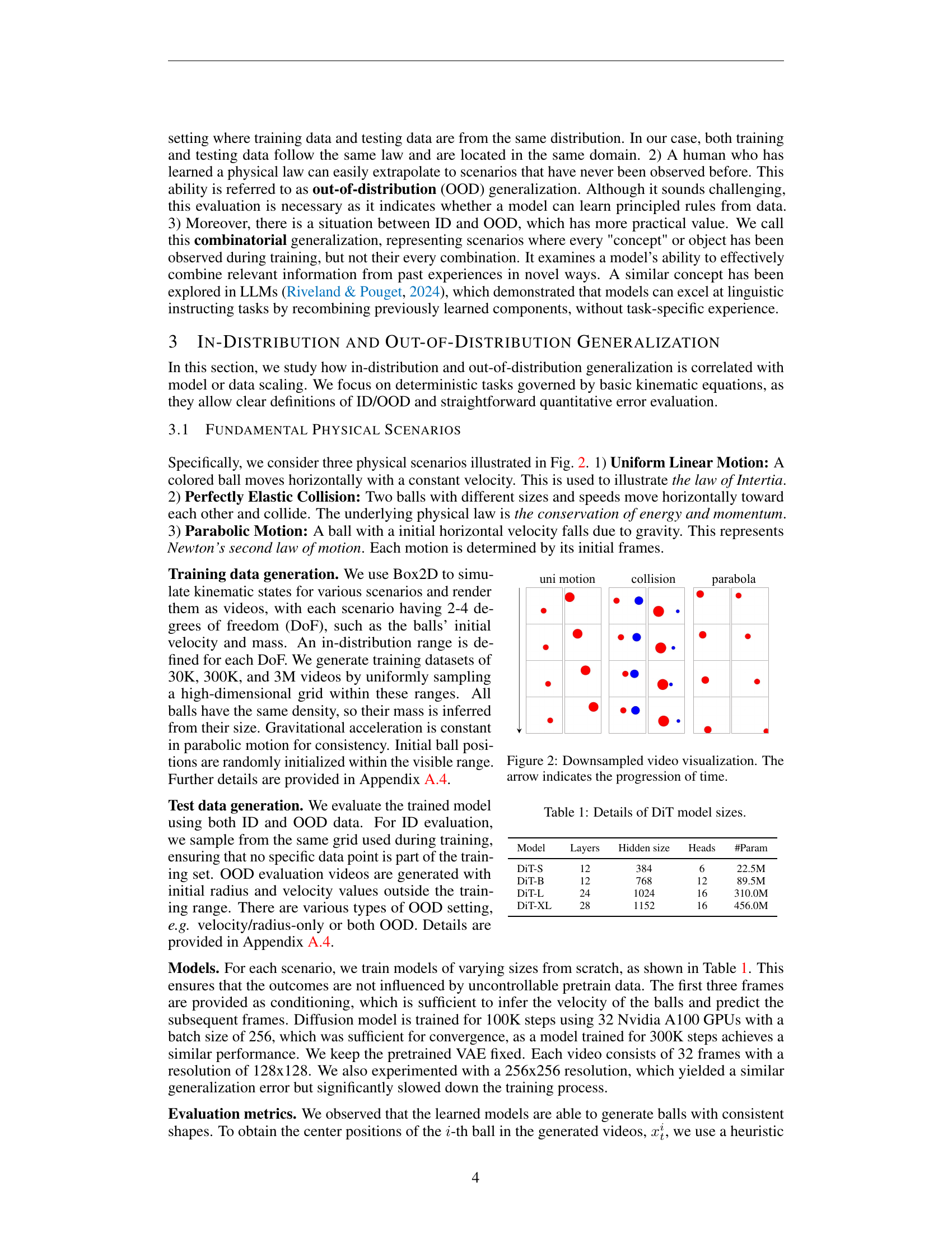
🔼 This figure visualizes downsampled videos from a 2D physics simulation used in the paper. Three distinct scenarios are shown, each demonstrating a different fundamental physical law: 1) Uniform Linear Motion (a ball moving at a constant velocity), 2) Perfectly Elastic Collision (two balls colliding), and 3) Parabolic Motion (a ball following a parabolic trajectory due to gravity). The arrow in each video segment indicates the progression of time, showing the evolution of the physical system. The figure is a simplified representation to facilitate quantitative evaluation of video generation models’ ability to learn and extrapolate physical laws.
read the caption
Figure 2: Downsampled video visualization. The arrow indicates the progression of time.

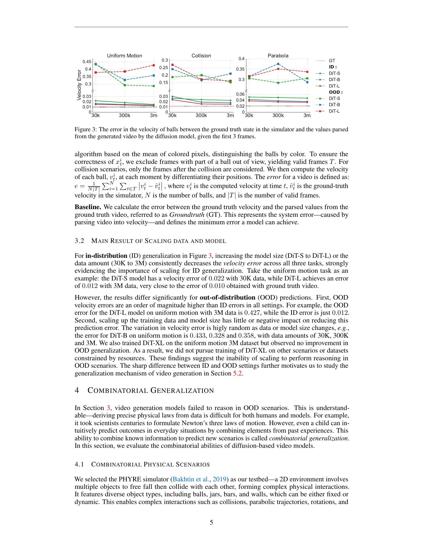
🔼 This figure displays the velocity error for three different physical scenarios (Uniform Motion, Collision, Parabola) across various model and dataset sizes. The velocity error represents the difference between the actual velocity of the balls calculated from the simulator’s ground truth and the velocity estimated from the video generated by the diffusion model. The first three frames of each video serve as input to the model. The results show how the model’s velocity prediction accuracy changes with the scale of both the model and training data.
read the caption
Figure 3: The error in the velocity of balls between the ground truth state in the simulator and the values parsed from the generated video by the diffusion model, given the first 3 frames.

🔼 This figure visualizes example videos from a 2D physics simulation used in the paper. Each video shows multiple objects with various shapes and colors interacting under the influence of gravity and collisions. Black objects represent fixed elements in the environment, while other objects (red ball and others) are dynamic and move according to the laws of physics. The videos serve to demonstrate the complexity of the physical interactions that the model must learn from and make predictions about.
read the caption
Figure 4: Downsampled videos. The black objects are fixed and others are dynamic.

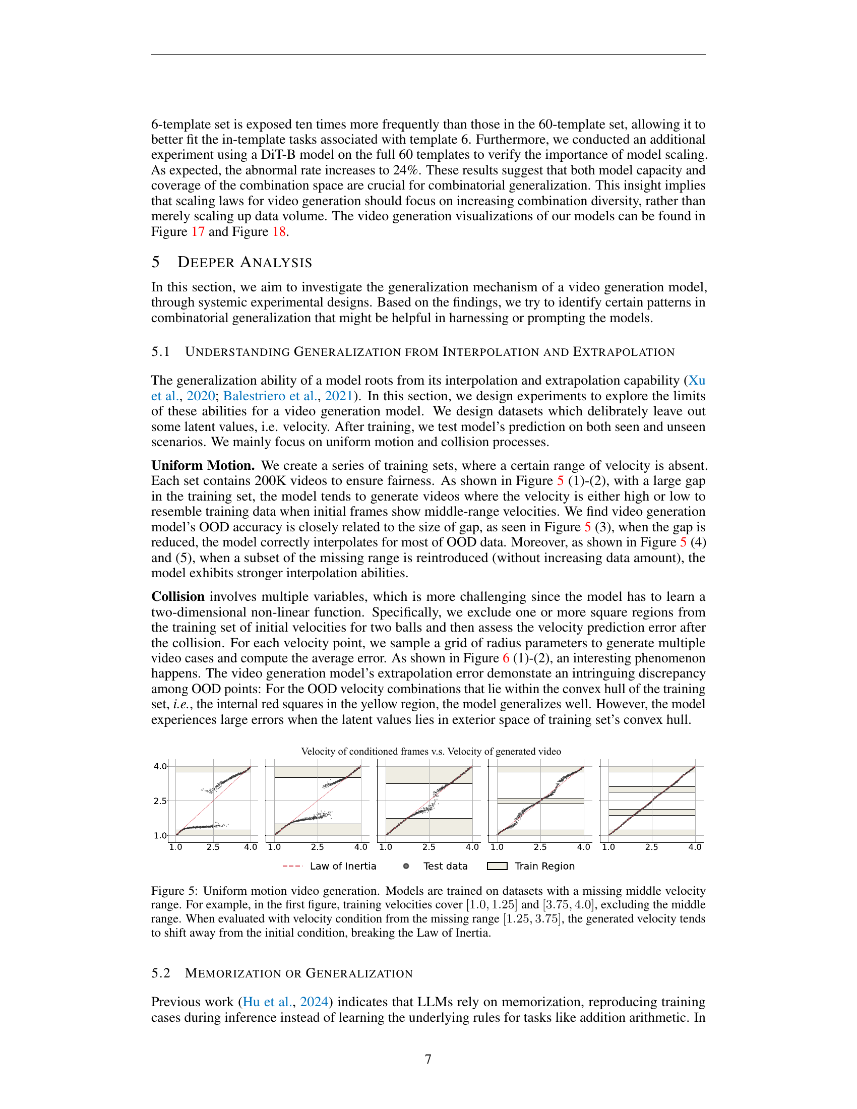
🔼 This figure demonstrates the limitations of video generation models when extrapolating beyond their training data. The experiment focuses on uniform linear motion of a ball, a simple physical phenomenon governed by Newton’s First Law of Motion (Inertia). Multiple models are trained on datasets where a range of velocities are intentionally omitted (the ‘missing middle velocity range’). When the model is then tested with velocities within this missing range, it fails to correctly predict the constant velocity, instead generating videos where the velocity deviates significantly from the expected constant value, violating the Law of Inertia. This demonstrates a ‘case-based’ generalization approach rather than true understanding of the physical law. The model appears to ‘mimic’ the closest training example rather than extrapolate based on a learned principle.
read the caption
Figure 5: Uniform motion video generation. Models are trained on datasets with a missing middle velocity range. For example, in the first figure, training velocities cover [1.0,1.25]1.01.25[1.0,1.25][ 1.0 , 1.25 ] and [3.75,4.0]3.754.0[3.75,4.0][ 3.75 , 4.0 ], excluding the middle range. When evaluated with velocity condition from the missing range [1.25,3.75]1.253.75[1.25,3.75][ 1.25 , 3.75 ], the generated velocity tends to shift away from the initial condition, breaking the Law of Inertia.

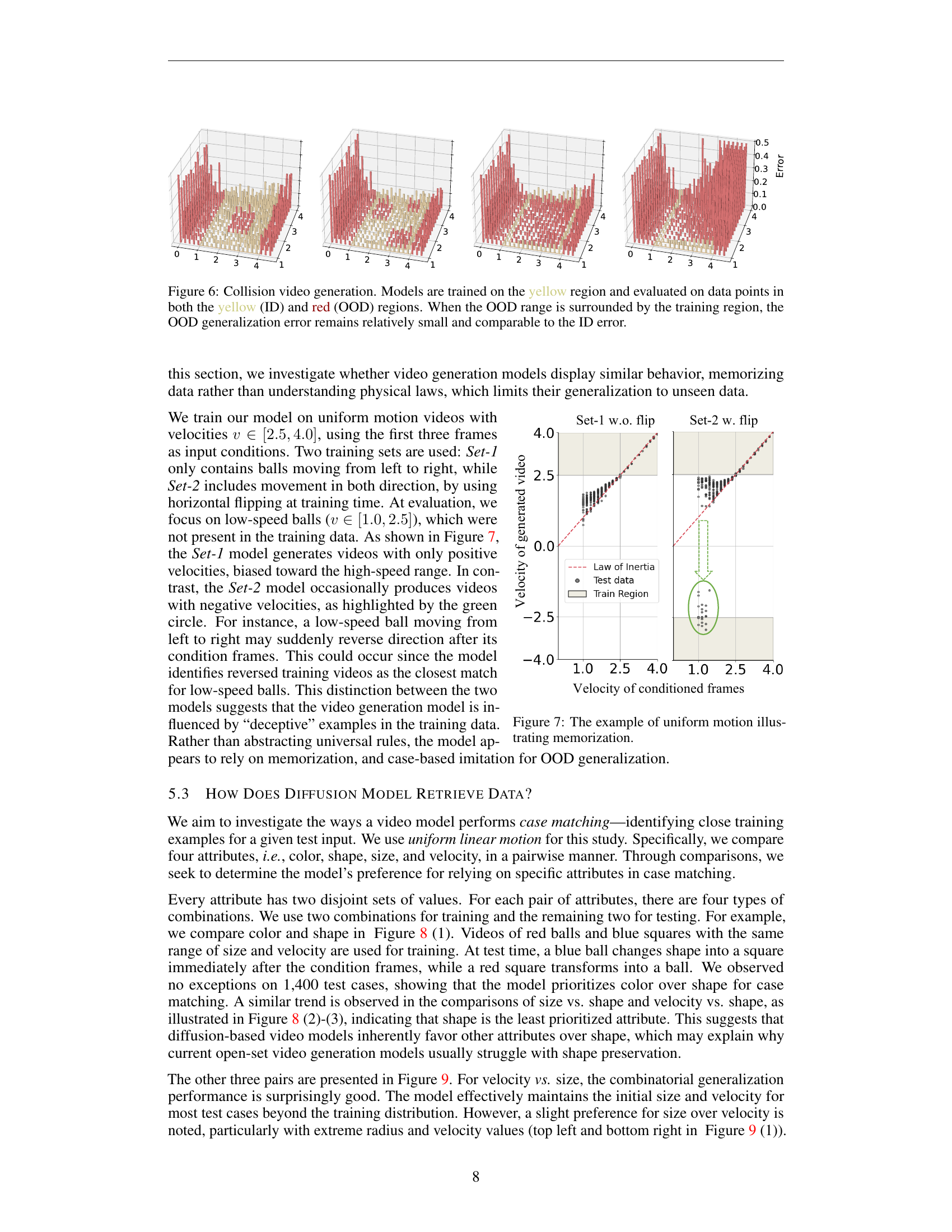
🔼 This figure visualizes the results of collision video generation experiments. The models were trained using data within the yellow region. Then, they were evaluated on data points both inside the yellow region (in-distribution, or ID) and the red region (out-of-distribution, or OOD). The key finding highlighted is that when the OOD data points are surrounded by the training data, the generalization error for the OOD data remains low and similar to the error for the ID data. This suggests that the model’s ability to generalize to unseen scenarios is related to the proximity of those scenarios to the training data.
read the caption
Figure 6: Collision video generation. Models are trained on the yellow region and evaluated on data points in both the yellow (ID) and red (OOD) regions. When the OOD range is surrounded by the training region, the OOD generalization error remains relatively small and comparable to the ID error.

🔼 This figure demonstrates the model’s memorization behavior during generalization. The model was trained on videos of uniform linear motion with velocities in the range of 2.5 to 4.0 units. It was trained on two datasets: one only containing objects moving in one direction, and another containing movements in both directions, achieved by horizontal flipping during training. During testing, the model was given low-speed objects (velocity 1.0 to 2.5). The results show that a model trained only on one direction generated videos with velocities biased toward the higher range and only in the trained direction. In contrast, the model trained with both directions occasionally produced videos moving in the opposite direction, showcasing the model’s tendency to ‘memorize’ training examples rather than learn the underlying physical law of uniform motion.
read the caption
Figure 7: The example of uniform motion illustrating memorization.

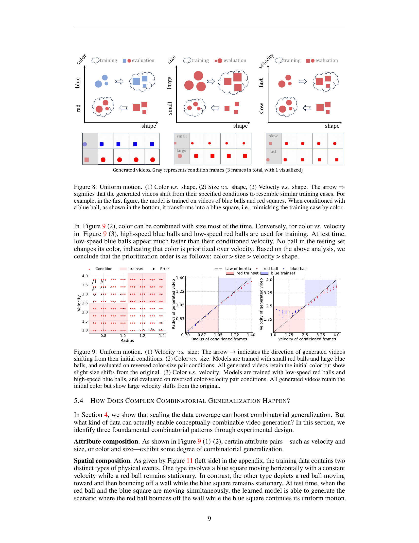
🔼 This figure demonstrates how a video generation model generalizes based on different attributes (color, size, and velocity) when dealing with shape. It shows three experiments comparing pairs of these attributes. In each experiment, the model is trained on videos featuring two distinct combinations of attributes. The model is then tested with videos that combine the attributes in novel ways. Arrows indicate that the generated videos tend to shift their visual properties from the testing data’s initial conditions to more closely resemble similar training examples. For instance, in the first experiment comparing color and shape, when trained on red squares and blue balls and tested with a blue ball, the model changes the ball into a blue square.
read the caption
Figure 8: Uniform motion. (1) Color v.s. shape, (2) Size v.s. shape, (3) Velocity v.s. shape. The arrow ⇒⇒\Rightarrow⇒ signifies that the generated videos shift from their specified conditions to resemble similar training cases. For example, in the first figure, the model is trained on videos of blue balls and red squares. When conditioned with a blue ball, as shown in the bottom, it transforms into a blue square, i.e., mimicking the training case by color.

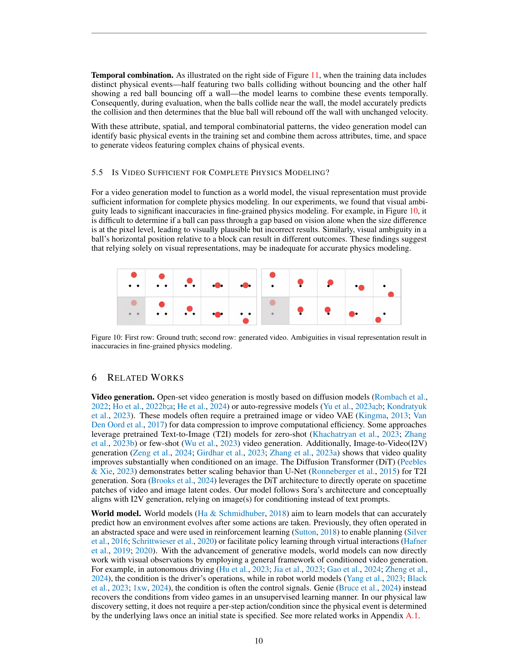
🔼 Figure 9 presents a detailed analysis of how a video generation model generalizes based on various attributes. It explores three scenarios, each comparing two attributes: (1) Velocity vs. Size: The model’s predictions are shown when presented with initial conditions outside its training data. The arrows indicate the direction of the generated video’s velocity changing from the initial state. (2) Color vs. Size: The model is trained on videos featuring small red balls and large blue balls. Testing is performed on reversed conditions (large red balls and small blue balls). Results show that generated videos generally maintain the initial color but often exhibit size variations. (3) Color vs. Velocity: Similar to (2), training uses low-speed red balls and high-speed blue balls, with testing on reversed conditions. Generated videos preserve the initial color but demonstrate significant discrepancies in velocity compared to the initial conditions. This figure helps explain how the model’s generalization process favors specific attributes over others.
read the caption
Figure 9: Uniform motion. (1) Velocity v.s. size: The arrow →→\rightarrow→ indicates the direction of generated videos shifting from their initial conditions. (2) Color v.s. size: Models are trained with small red balls and large blue balls, and evaluated on reversed color-size pair conditions. All generated videos retain the initial color but show slight size shifts from the original. (3) Color v.s. velocity: Models are trained with low-speed red balls and high-speed blue balls, and evaluated on reversed color-velocity pair conditions. All generated videos retain the initial color but show large velocity shifts from the original.

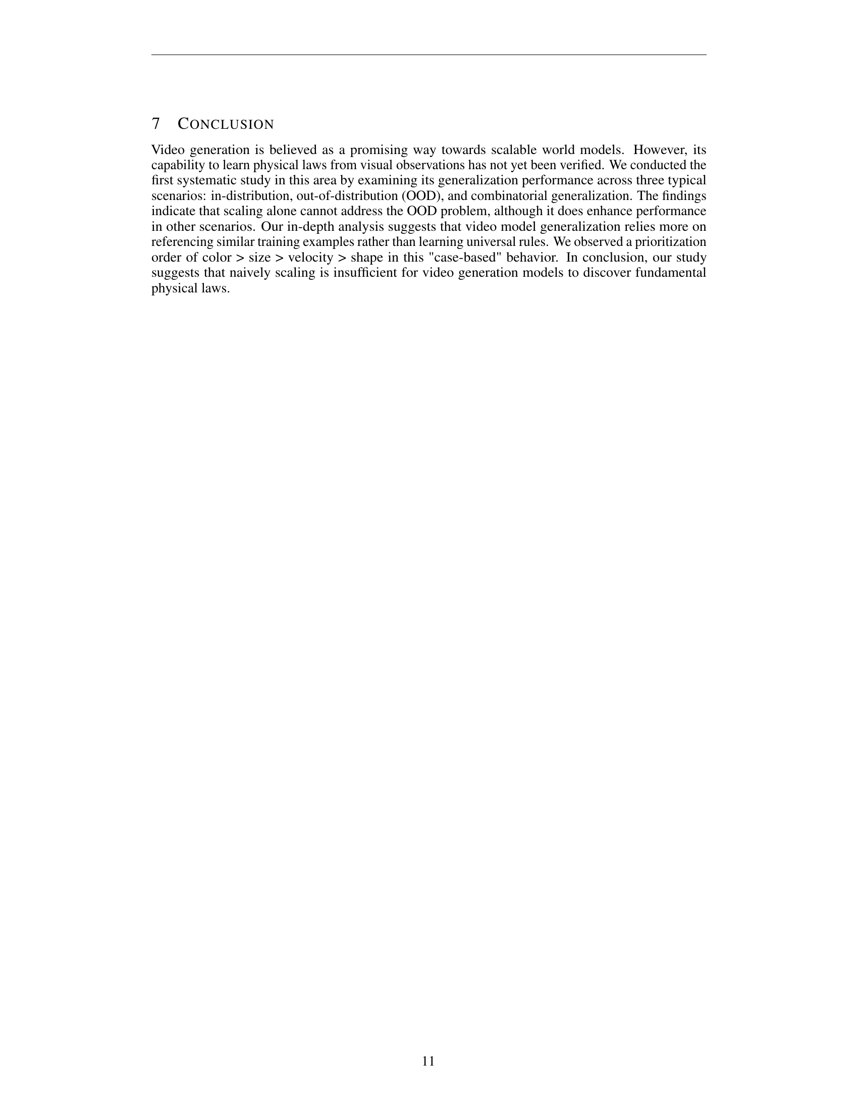
🔼 This figure demonstrates the limitations of relying solely on visual information for accurate physics modeling in video generation. The top row shows the ground truth frames of a video, while the bottom row displays the corresponding frames generated by a video generation model. The subtle differences between the ground truth and generated video highlight a key problem: when fine-grained details, like the exact position of a ball relative to a gap, are visually ambiguous, the model produces plausible-looking but inaccurate results. This indicates that visual information alone may be insufficient for precise physical modeling, particularly in scenarios involving subtle spatial relationships.
read the caption
Figure 10: First row: Ground truth; second row: generated video. Ambiguities in visual representation result in inaccuracies in fine-grained physics modeling.

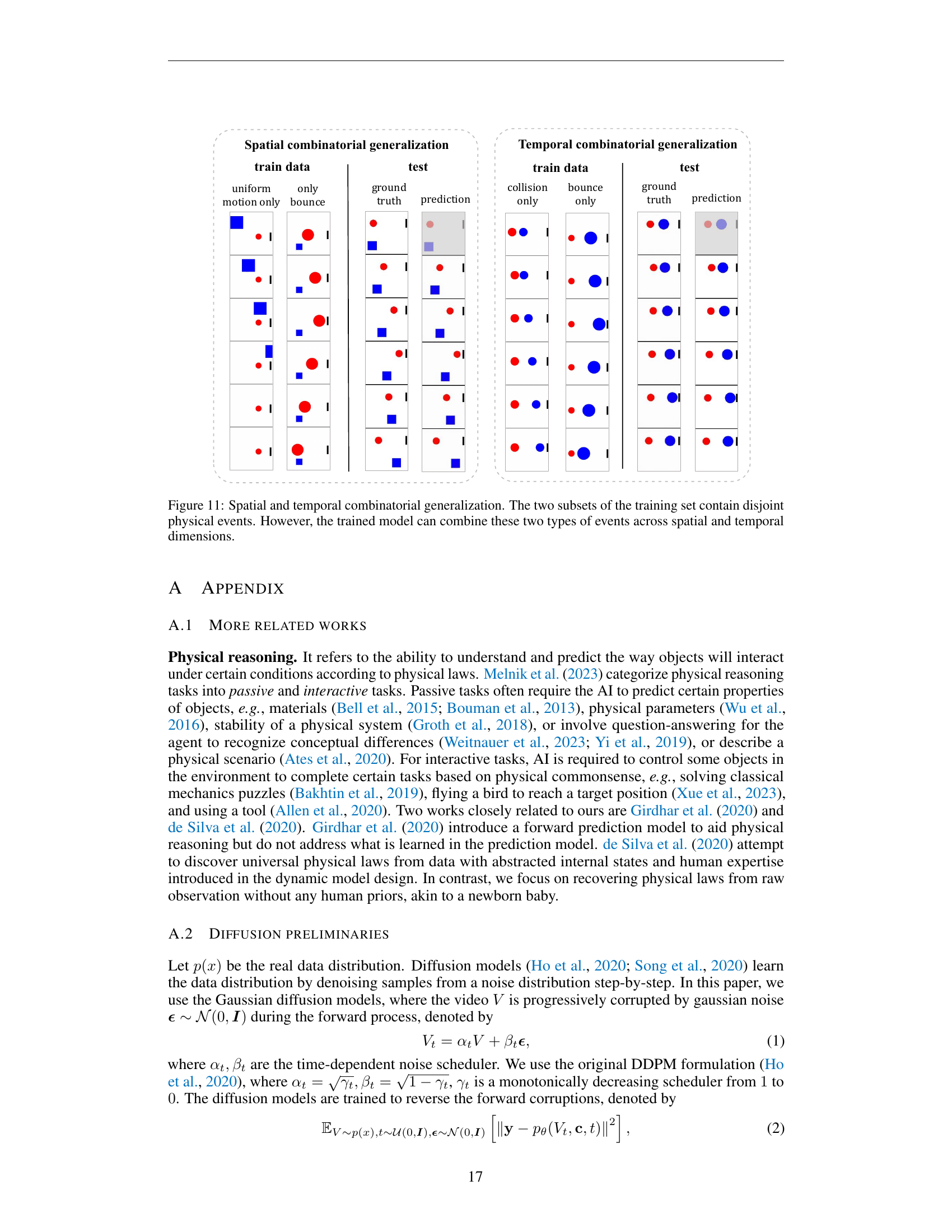
🔼 Figure 11 demonstrates the model’s ability to generalize beyond simple scenarios by combining elements from different situations in both space and time. The training data is divided into two sets: one showing a blue square moving horizontally while a red ball remains stationary, and another showing a red ball bouncing off a wall while a blue square is stationary. Importantly, these scenarios are distinct; the model was never shown both events happening simultaneously. However, when presented with a test scenario where both events occur (the blue square moves horizontally, and the red ball bounces), the model correctly predicts the combined outcome. This shows the model is not simply memorizing training examples but can synthesize new behaviors by integrating disparate learned skills.
read the caption
Figure 11: Spatial and temporal combinatorial generalization. The two subsets of the training set contain disjoint physical events. However, the trained model can combine these two types of events across spatial and temporal dimensions.

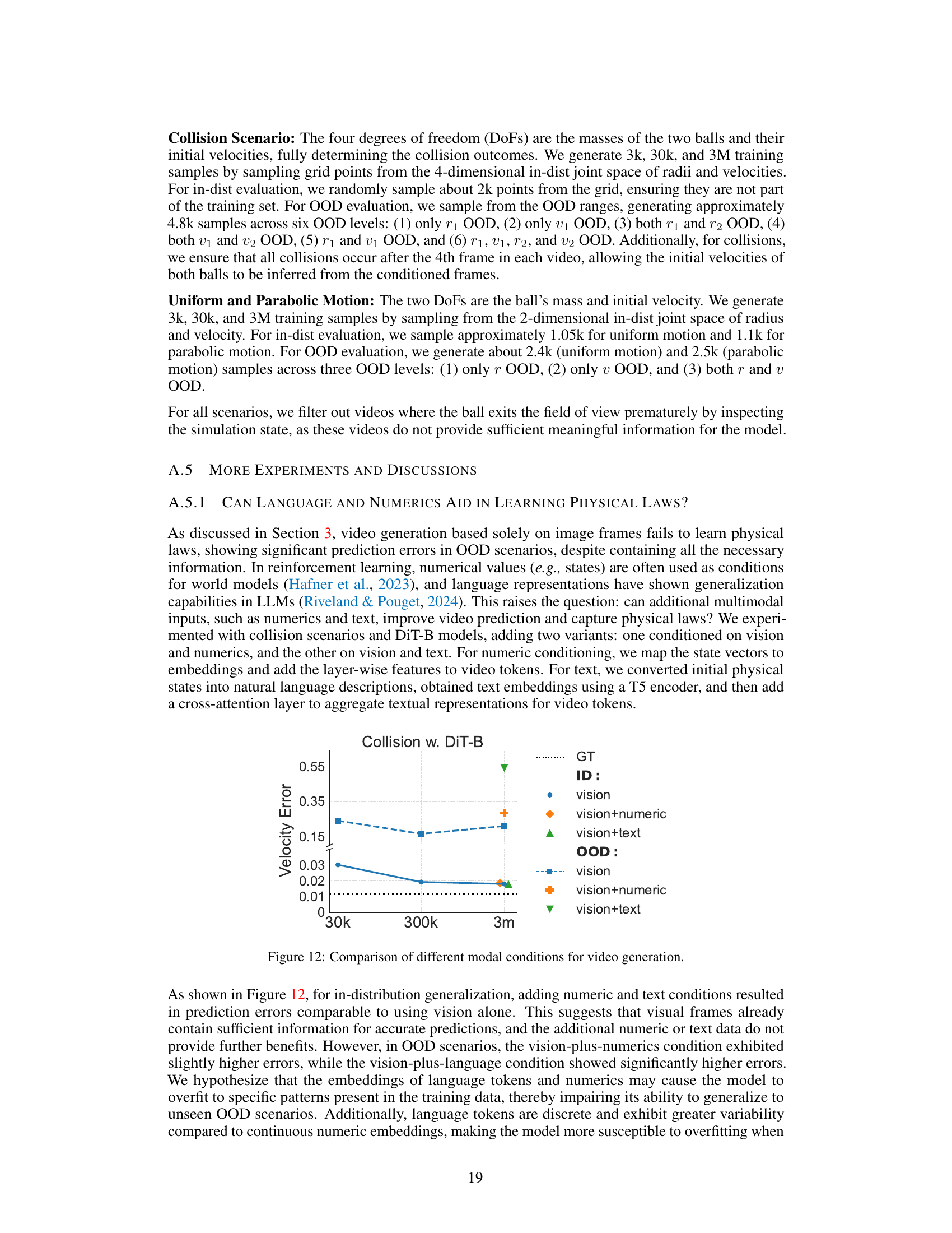
🔼 This figure displays a comparison of video generation results under different input conditions. It shows velocity error as a function of training data size, contrasting results when the model is conditioned only on visual data, visual data plus numerical data, and visual data plus textual descriptions. The goal is to assess whether incorporating additional information like numbers or text improves physical law learning and generalization to out-of-distribution (OOD) scenarios.
read the caption
Figure 12: Comparison of different modal conditions for video generation.

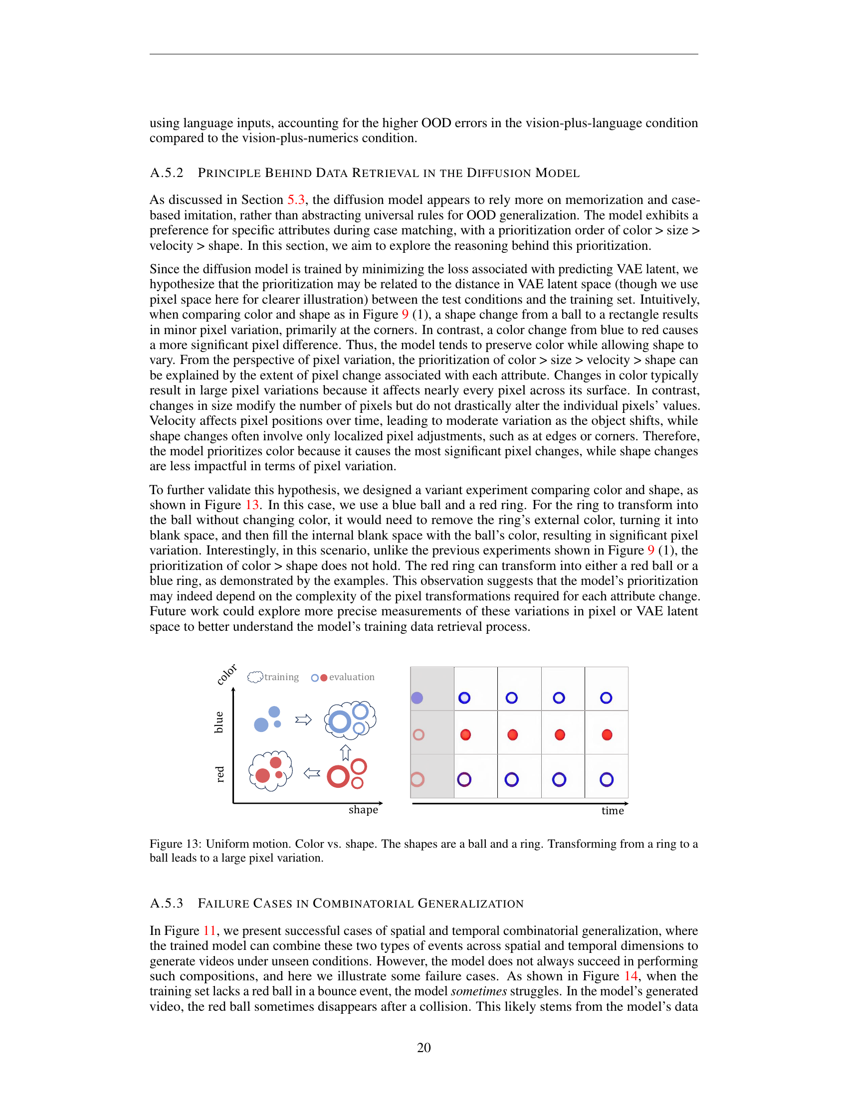
🔼 This figure demonstrates the effect of color and shape on a video generation model’s ability to generalize to unseen scenarios. The model is trained on videos showing red squares and blue balls moving uniformly. During testing, the model is conditioned on frames showing a blue ring. Because the model prioritizes color, it transforms the blue ring into a blue ball instead of preserving the shape of the ring. This highlights the model’s reliance on visual similarities rather than underlying physical laws in its generalization. The caption emphasizes the large pixel variation involved in changing a ring into a ball, suggesting this is a factor contributing to the model’s reliance on color in its decision-making process.
read the caption
Figure 13: Uniform motion. Color vs. shape. The shapes are a ball and a ring. Transforming from a ring to a ball leads to a large pixel variation.

🔼 Figure 14 illustrates instances where the model fails to generalize combinatorially. The model struggles to produce videos with the expected outcomes when presented with test scenarios that combine elements not seen together during training. Specifically, the training data included scenarios with bouncing balls but excluded cases where a red ball bounced. Consequently, when a test scenario involving a red ball bounce was presented, the model failed to correctly predict the resulting video. The failure highlights the model’s reliance on memorizing specific training examples rather than learning generalizable rules about physics.
read the caption
Figure 14: Failure cases in combinatorial generalization. Note that the bounce cases in the training set do not include the red ball.

🔼 Figure 15 visualizes several example video sequences generated by the model for in-distribution testing scenarios. Each example demonstrates successful prediction of object motion, indicating that the model accurately captures the underlying physical laws within its training data distribution. The videos showcase scenarios of uniform linear motion, perfectly elastic collisions, and parabolic motion, all of which are accurately predicted by the model. The close alignment between the generated videos and ground truth in these examples signifies strong in-distribution generalization capability. The model’s accurate prediction of these simple physical phenomena is a crucial aspect of its overall physical law discovery ability. The precise matching between generated and ground truth videos in Figure 15 provides strong evidence of the model’s capability to learn and apply physical laws within a constrained setting.
read the caption
Figure 15: The visualization of in-distribution evaluation cases with very small prediction errors.

🔼 This figure visualizes examples from the out-of-distribution (OOD) test set where the model’s predictions significantly deviate from the ground truth. It showcases instances of uniform linear motion, collision, and parabolic motion where the model fails to accurately predict the velocity or trajectory of the objects, resulting in large prediction errors. The visualization helps illustrate the model’s limitations in generalizing to unseen scenarios outside the training distribution.
read the caption
Figure 16: The visualization of out-of-distribution evaluation cases with large prediction errors.

🔼 Figure 17 visualizes the results of out-of-template evaluation of a video generation model (DiT-XL). The model was trained on 6 million video samples representing 60 unique scenarios (templates). The figure shows several video examples where the model generated videos which are visually very similar to the actual ground truth videos, thus appearing plausible and obeying physical laws. However, while many of the generated videos are near-perfect matches, there are cases (like the rightmost example) where minor visual discrepancies exist between the generated video and the ground truth. These discrepancies, while visually subtle, indicate that the model hasn’t perfectly captured and replicated the underlying physical process, highlighting the limitations of using visual information alone for learning physical laws (further elaborated in Section 5.5).
read the caption
Figure 17: The visualization of out-of-template evaluation cases that appear plausible and adhere to physical laws, generated by DiT-XL trained on 6M data (60 templates). Zoom in for details. Notably, the first four cases generated by the model are nearly identical to the ground truth. In some cases, such as the rightmost example, the generated video seems physically plausible but differs from the ground truth due to visual ambiguity, as discussed in Section 5.5.
More on tables
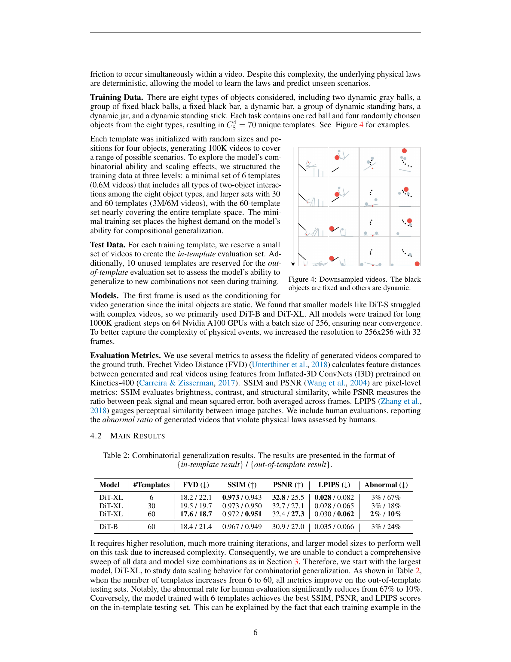
| Model | #Templates | FVD (↓) | SSIM (↑) | PSNR (↑) | LPIPS (↓) | Abnormal (↓) |
|---|---|---|---|---|---|---|
| DiT-XL | 6 | 18.2 / 22.1 | 0.973 / 0.943 | 32.8 / 25.5 | 0.028 / 0.082 | 3% / 67% |
| DiT-XL | 30 | 19.5 / 19.7 | 0.973 / 0.950 | 32.7 / 27.1 | 0.028 / 0.065 | 3% / 18% |
| DiT-XL | 60 | 17.6 / 18.7 | 0.972 / 0.951 | 32.4 / 27.3 | 0.030 / 0.062 | 2% / 10% |
| DiT-B | 60 | 18.4 / 21.4 | 0.967 / 0.949 | 30.9 / 27.0 | 0.035 / 0.066 | 3% / 24% |
🔼 This table presents the results of evaluating combinatorial generalization in video generation models. It shows the performance of models on both in-distribution (in-template) and out-of-distribution (out-of-template) generalization tasks. The metrics used to evaluate the model’s performance are Frechet Video Distance (FVD), Structural Similarity Index (SSIM), Peak Signal-to-Noise Ratio (PSNR), Learned Perceptual Image Patch Similarity (LPIPS), and the percentage of generated videos deemed ‘abnormal’ by human evaluators. The results are presented in a format showing in-template scores followed by a slash and then out-of-template scores for easier comparison.
read the caption
Table 2: Combinatorial generalization results. The results are presented in the format of {in-template result} / {out-of-template result}.
| Scenario | Ground Truth Error | VAE Reconstruction Error |
|---|---|---|
| Uniform Motion | 0.0099 | 0.0105 |
| Collision | 0.0117 | 0.0131 |
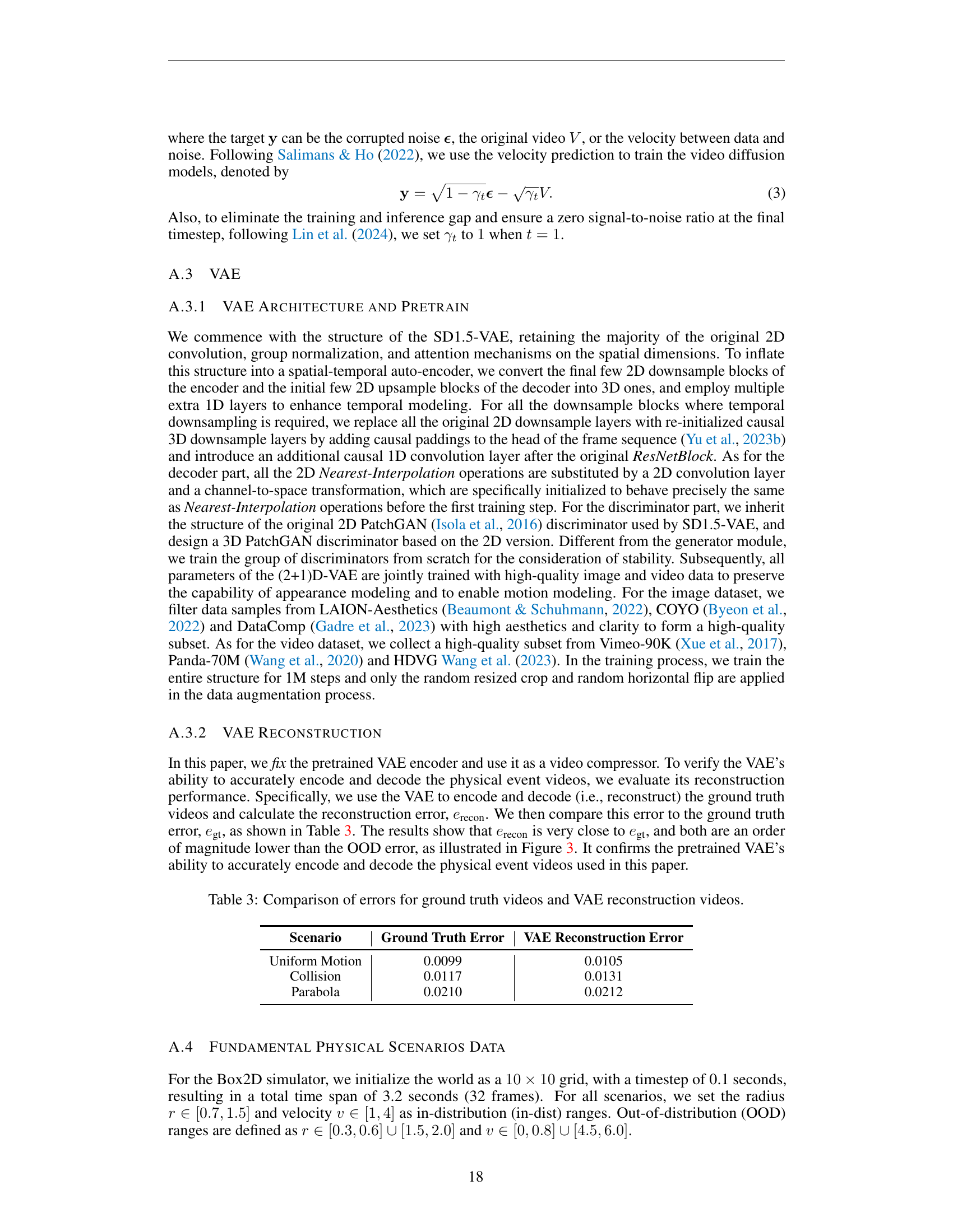
| Parabola | 0.0210 | 0.0212 |
🔼 This table presents a quantitative comparison of reconstruction errors between the ground truth videos and those reconstructed using a Variational Autoencoder (VAE). The goal is to demonstrate the VAE’s accuracy in encoding and decoding videos of physical events. The lower the reconstruction error (compared to the ground truth error), the better the VAE’s performance in capturing and reproducing the key information in the videos.
read the caption
Table 3: Comparison of errors for ground truth videos and VAE reconstruction videos.
Full paper#
