TL;DR#
Training large language models efficiently requires advanced parallel computing techniques, such as pipeline parallelism. However, current methods often suffer from imbalanced computation and memory usage across pipeline stages, leading to reduced efficiency. This imbalance is particularly pronounced in vocabulary layers, which are responsible for mapping words to their numerical representations. Existing solutions, like layer redistribution, have limited success and may even worsen the problem.
This research introduces Vocabulary Parallelism, a novel approach to overcome this limitation. By evenly distributing the vocabulary layers across pipeline devices and optimizing communication, the method effectively balances computation and memory usage. Experiments show significant performance gains (5%-51% improvement) with reduced memory consumption, especially for models with large vocabularies. The technique is also adaptable to various existing pipeline scheduling strategies, enhancing its practicality and potential impact on large-scale model training.
Key Takeaways#
Why does it matter?#
This paper is crucial for researchers working on large language model training because it addresses a significant bottleneck—imbalanced computation and memory usage in pipeline parallelism—that hinders scalability. The proposed Vocabulary Parallelism offers a practical solution, improving throughput and memory efficiency, and opens new avenues for optimizing parallel training across diverse model architectures. Its open-sourced implementation further enhances its value to the research community.
Visual Insights#

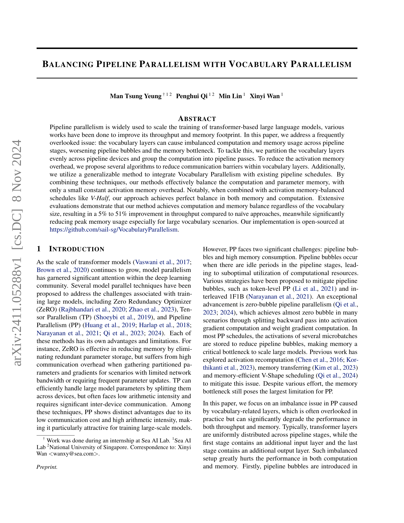
🔼 Figure 1 illustrates the repeating pattern of an imbalanced pipeline caused by an extra output layer in the final stage. This extra layer leads to an uneven distribution of workload across pipeline stages. The stages with fewer layers have less computation, creating idle time or ‘bubbles’ in the pipeline. This reduces overall efficiency and throughput.
read the caption
Figure 1: Repeating pattern in an imbalanced pipeline. Bubbles are incurred due to an extra output layer in the last pipeline stage.
| Pipelines (GPUs) | 8 | 16 | 32 |
|---|---|---|---|
| Model Size | ≈ 4B | ≈ 10B | ≈ 21B |
| Layers | 32 | 48 | 64 |
| Attention Heads | 24 | 32 | 40 |
| Hidden Size | 3072 | 4096 | 5120 |
| Sequence Length | 2048 / 4096 | 2048 / 4096 | 2048 / 4096 |
| Microbatch Size | 1 | 1 | 1 |
| Number of Microbatches | 128 | 128 | 128 |
| Vocabulary Size | 32k / 64k / 128k / 256k | 32k / 64k / 128k / 256k | 32k / 64k / 128k / 256k |
🔼 This table details the configurations used in the experiments based on the 1F1B pipeline scheduling. It lists the number of GPUs used, model sizes (approximate parameter count), number of layers, attention heads, hidden size, sequence length, microbatch size, number of microbatches, and vocabulary size for various experimental settings. This information is crucial for understanding the scale and scope of the experiments conducted in the study.
read the caption
Table 1: Settings used in experiments on 1F1B schedule.
In-depth insights#
Vocab Parallelism#
The concept of ‘Vocab Parallelism’ introduces a novel approach to address computational and memory imbalances in pipeline parallelism for large language model training. Vocabulary layers, often responsible for significant compute and memory overhead, are partitioned and distributed across multiple devices. This partitioning is crucial for balancing the workload, preventing the concentration of processing on a few devices, and minimizing pipeline bubbles. By employing algorithms that cleverly group computation and communication barriers, activation memory overhead is efficiently reduced. Further, the seamless integration of ‘Vocab Parallelism’ with existing pipeline schedules enhances overall training efficiency, achieving near-perfect balance in computation and memory. The method demonstrates remarkable improvements in throughput, significantly reducing peak memory consumption. This innovative approach proves particularly beneficial when dealing with very large vocabulary sizes, where the imbalance issue is most pronounced. The open-sourcing of the implementation facilitates wider adoption and further research in this crucial area of large language model optimization.
Pipeline Imbalance#
Pipeline imbalance in large language model training arises from uneven computational loads and memory usage across different pipeline stages. Vocabulary layers, often significantly larger than typical transformer layers, are a primary contributor, creating bottlenecks. This imbalance leads to pipeline bubbles, periods of inactivity in certain stages, reducing overall efficiency. The paper highlights how this imbalance is frequently overlooked, resulting in suboptimal performance. The uneven distribution of computational work affects throughput, while memory consumption is also impacted. Addressing this requires sophisticated strategies, such as Vocabulary Parallelism, which evenly distributes vocabulary layers across devices, mitigating both computation and memory imbalances. Careful scheduling of communication barriers within vocabulary layers is critical to avoid further reducing efficiency. The key takeaway is that achieving balanced resource utilization throughout the pipeline is crucial for optimal large language model training, and addressing vocabulary layer imbalance is essential to improve both memory efficiency and throughput.
Activation Memory#
Activation memory in large language model training is a critical bottleneck, especially when employing pipeline parallelism. The sheer volume of intermediate activations generated during forward and backward passes can overwhelm GPU memory, leading to performance degradation or complete failure. Strategies to mitigate this include activation recomputation, trading off computation time for reduced memory footprint. Another approach is memory-efficient scheduling, such as V-Shape scheduling, which carefully orchestrates the flow of data to minimize peak memory usage. However, these methods often don’t fully address the problem, especially when dealing with imbalanced computation across pipeline stages, a common issue in vocabulary layers. Effectively balancing activation memory requires sophisticated scheduling and resource allocation to ensure efficient utilization of GPU resources without compromising training speed or model accuracy. Therefore, new techniques for activation memory management remain a crucial area of research for scaling large language model training effectively.
Scheduling Methods#
Effective pipeline parallelism in large language model training hinges on efficient scheduling methods. The core challenge lies in balancing computation and memory across pipeline stages, which are often unevenly loaded due to variations in layer complexity and the presence of vocabulary layers. Naive approaches that simply redistribute layers may not address the underlying imbalance. The paper explores sophisticated scheduling techniques like 1F1B and V-Half, which aim to minimize pipeline bubbles and memory consumption, but these are often insufficient when dealing with imbalanced workloads. Therefore, the authors propose a novel Vocabulary Parallelism scheme to specifically tackle the uneven distribution of computational costs and memory requirements in vocabulary layers. This involves partitioning vocabulary layers across devices and integrating them into existing pipeline schedules in a memory-efficient way, carefully managing communication barriers to reduce overhead. The integration is designed to be relatively independent of the base schedule, making it compatible with a range of techniques, and potentially leading to improved throughput and reduced memory usage, especially for models with large vocabularies.
Scalability Analysis#
A robust scalability analysis of vocabulary parallelism within pipeline parallelism is crucial for evaluating its effectiveness in training large language models. The analysis should quantify the impact of vocabulary size on both throughput and memory consumption, ideally across various model sizes and hardware configurations. It’s vital to compare the achieved scalability against an ideal linear scaling scenario, identifying potential bottlenecks or performance limitations. Detailed measurements of communication overhead (all-reduce operations, etc.) are necessary to determine the efficiency of the proposed vocabulary partitioning strategy. The effect of vocabulary size on peak memory usage needs careful examination, differentiating between parameter and activation memory. Furthermore, a strong scalability analysis would include a discussion of how the proposed methods scale with the number of devices (GPUs), assessing if performance improvements hold across different cluster sizes. Finally, an analysis of the trade-offs between communication costs, computation time, and memory usage is key to understanding the practical benefits and limitations of the proposed approach.
More visual insights#
More on figures

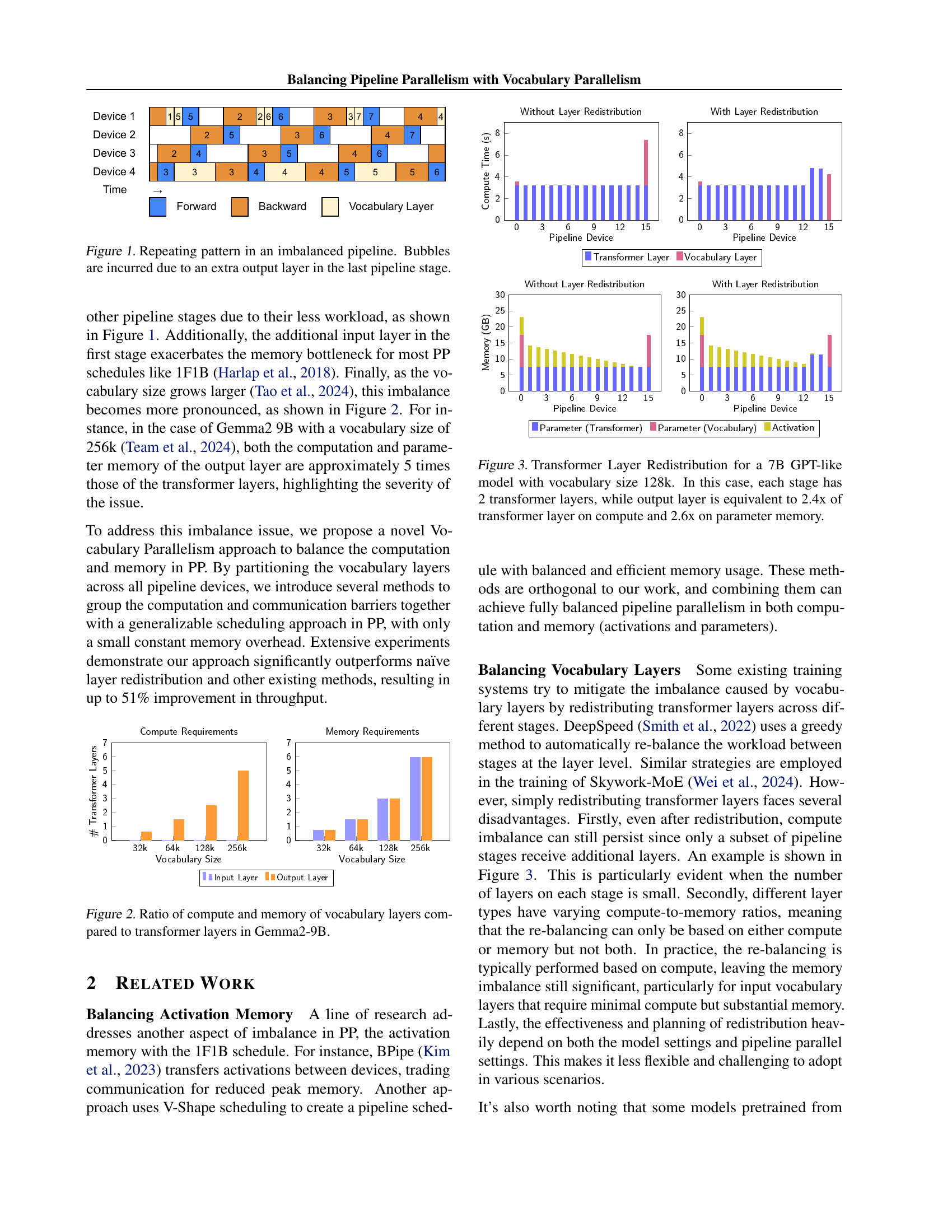
🔼 This figure shows a comparison of the computational and memory requirements of vocabulary layers relative to transformer layers in the Gemma2-9B language model. It illustrates how the compute and memory demands of the vocabulary layers scale significantly with increasing vocabulary size, underscoring the memory imbalance issue highlighted in the paper. This imbalance is more pronounced in larger vocabulary scenarios, demonstrating the need for the proposed Vocabulary Parallelism method.
read the caption
Figure 2: Ratio of compute and memory of vocabulary layers compared to transformer layers in Gemma2-9B.

🔼 This figure illustrates how transformer layers are redistributed in a 7B parameter GPT-like model with a vocabulary size of 128k to balance the computational load across pipeline stages. The redistribution aims to mitigate the imbalance caused by the vocabulary layers, which typically have disproportionately high computational and memory requirements compared to the transformer layers. The bar chart visually represents the compute requirements (in terms of time) and memory usage (parameter memory and activation memory) for each pipeline stage. We can observe that, after redistribution, each stage has roughly two transformer layers, ensuring a relatively even distribution of workload, while the output layer remains slightly more computationally expensive than an average transformer layer.
read the caption
Figure 3: Transformer Layer Redistribution for a 7B GPT-like model with vocabulary size 128k. In this case, each stage has 2 transformer layers, while output layer is equivalent to 2.4x of transformer layer on compute and 2.6x on parameter memory.

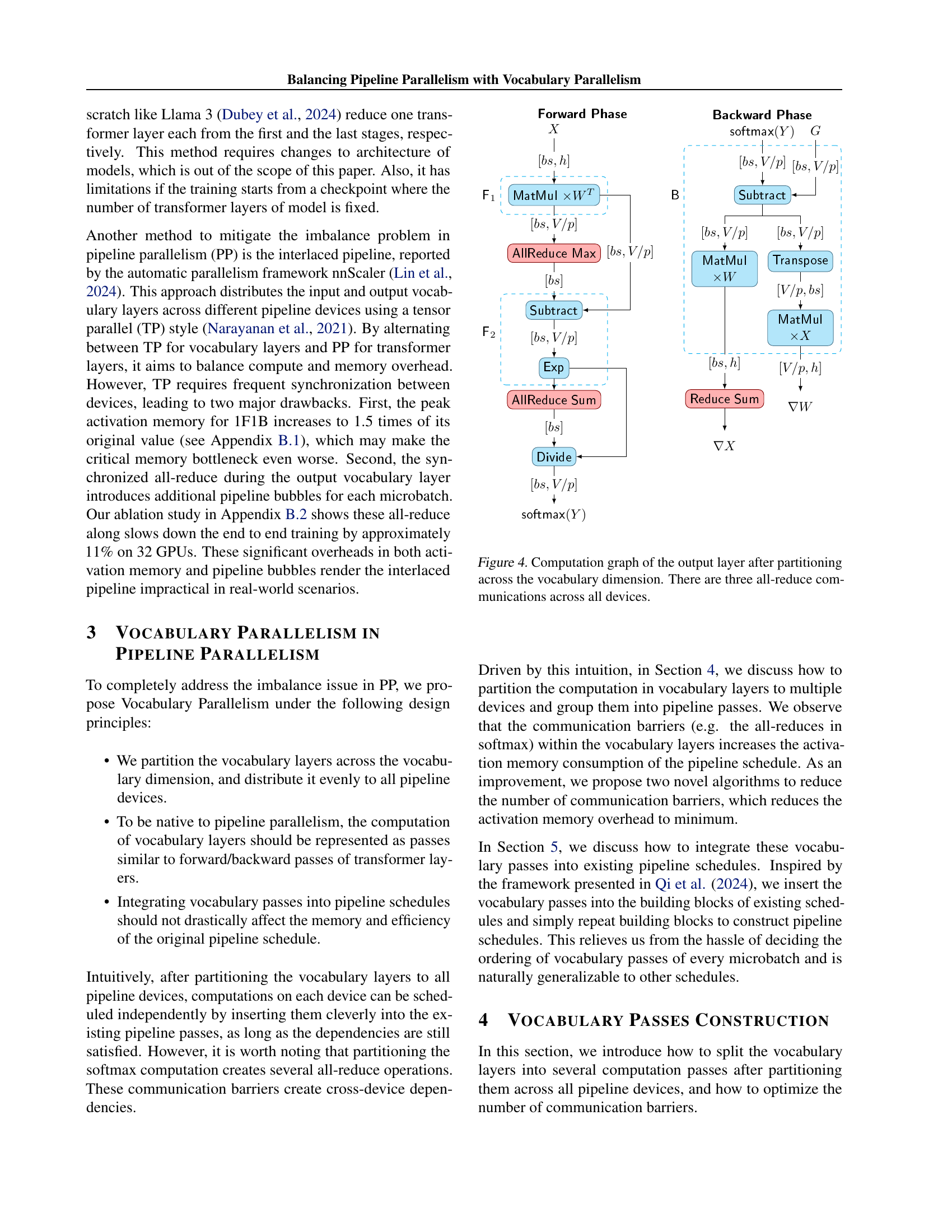
🔼 This figure illustrates the computation graph of the output layer after it’s been partitioned across multiple devices based on the vocabulary dimension. The process involves three steps. First, each device performs a matrix multiplication independently. Second, the maximum and sum of logits are computed via all-reduce operations, which require communication between all devices. Finally, the softmax function is calculated, followed by another all-reduce, and the weight gradient is computed. This highlights how the vocabulary layer’s parallelization introduces significant communication overhead.
read the caption
Figure 4: Computation graph of the output layer after partitioning across the vocabulary dimension. There are three all-reduce communications across all devices.

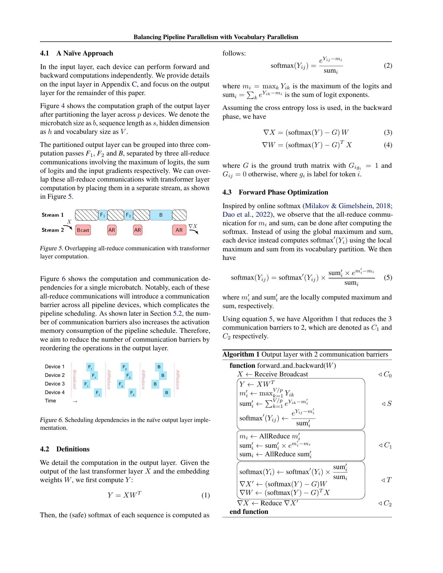
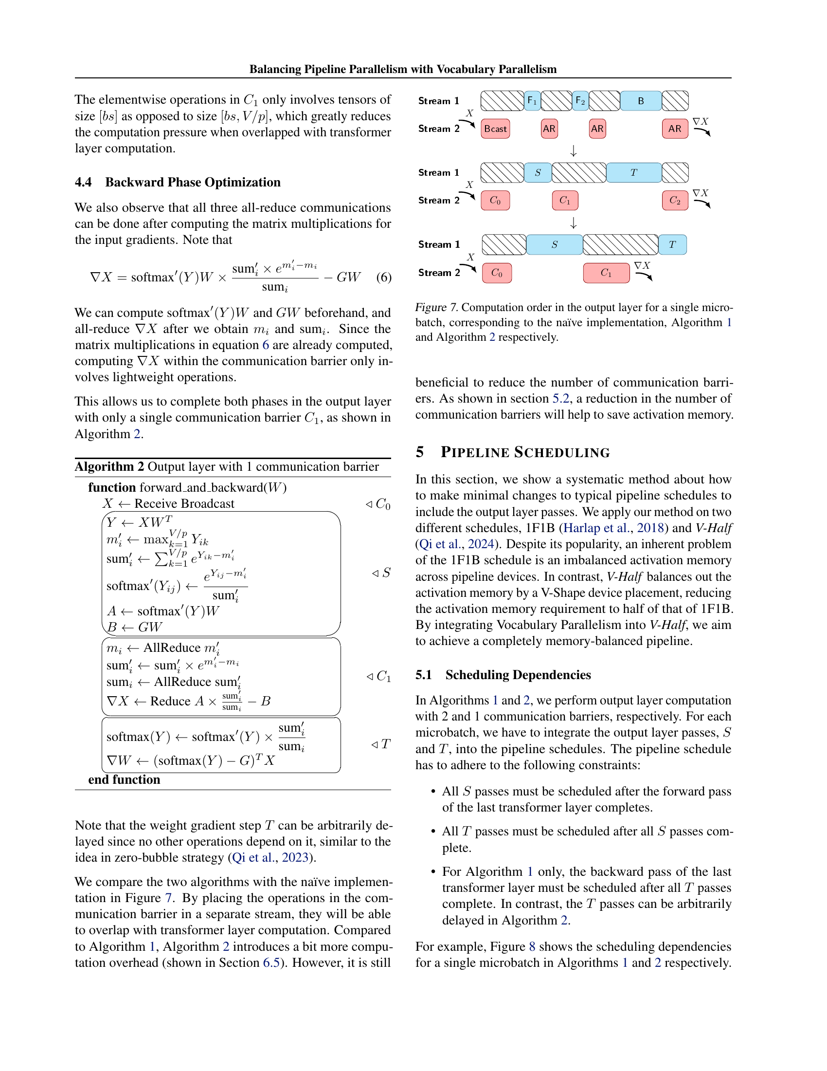
🔼 This figure illustrates how the all-reduce communication barriers inherent in the vocabulary layer computations can be overlapped with the computations of the transformer layers. By strategically placing these communications in a separate stream (Stream 2), as shown in the figure, the idle time caused by waiting for all-reduce operations is minimized, thereby improving the overall efficiency of the pipeline. Stream 1 shows transformer layer computations, while Stream 2 depicts all-reduce operations within the vocabulary layer. This technique is crucial in balancing pipeline parallelism with vocabulary parallelism, leading to reduced activation memory overhead and enhanced throughput.
read the caption
Figure 5: Overlapping all-reduce communication with transformer layer computation.

🔼 This figure illustrates the computational and communication dependencies in a naive implementation of the output layer, specifically focusing on the impact of partitioning the layer across multiple devices within a pipeline parallel system. The figure visually demonstrates how all-reduce communication barriers between devices, arising from operations like computing the maximum and sum of logits, create sequential dependencies that hinder efficient parallel processing and can lead to increased activation memory consumption. Each box represents a computational operation or communication barrier, and the arrows depict dependencies and the flow of data. The figure highlights the need for optimization strategies (as presented in later sections of the paper) to reduce or eliminate these communication barriers and improve the efficiency of the pipeline parallel system.
read the caption
Figure 6: Scheduling dependencies in the naïve output layer implementation.

🔼 Figure 7 illustrates the computation flow within the output layer for a single microbatch, comparing three different approaches: the naive method, Algorithm 1, and Algorithm 2. It highlights how each algorithm handles the computation and communication dependencies (specifically all-reduce operations) within the output layer to improve efficiency. The figure shows the order in which the computational steps (F1, F2, B, etc.) and communication steps (broadcast and all-reduce) are executed. It visualizes the differences in computational flow and barrier locations resulting from various optimization strategies implemented in Algorithms 1 and 2, contrasted with the naive approach.
read the caption
Figure 7: Computation order in the output layer for a single microbatch, corresponding to the naïve implementation, Algorithm 1 and Algorithm 2 respectively.

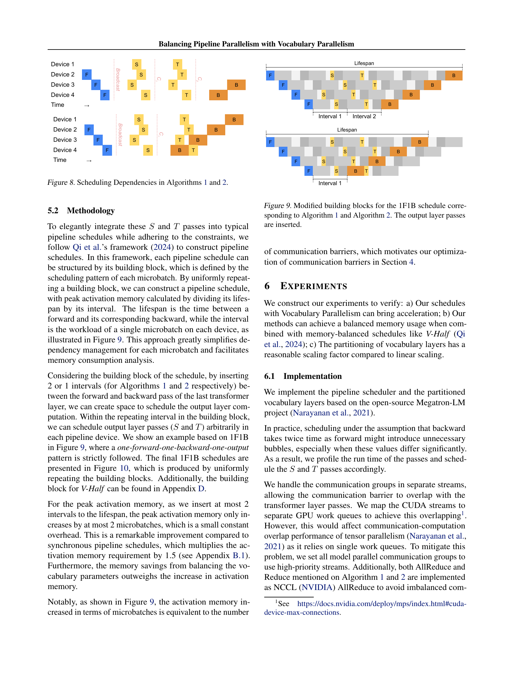
🔼 Figure 8 illustrates the scheduling dependencies for a single microbatch using Algorithms 1 and 2, which are methods for optimizing the output layer in pipeline parallelism. Algorithm 1 introduces two communication barriers (C1 and C2), while Algorithm 2 optimizes to only one barrier (C1). The figure shows how the forward (F) and backward (B) passes of the transformer layer interact with the vocabulary layer passes (S and T) within each algorithm. It highlights the dependencies between these passes and demonstrates how the number of communication barriers impacts the overall scheduling.
read the caption
Figure 8: Scheduling Dependencies in Algorithms 1 and 2.
More on tables
| Pipelines (GPUs) | 16 | 24 | 32 |
|---|---|---|---|
| Model Size | ≈ 7B | ≈ 16B | ≈ 30B |
| Layers | 32 | 48 | 64 |
| Attention Heads | 32 | 40 | 48 |
| Hidden Size | 4096 | 5120 | 6144 |
| Sequence Length | 2048 / 4096 | 2048 / 4096 | 2048 / 4096 |
| Microbatch Size | 1 | 1 | 1 |
| Number of Microbatches | 128 | 128 | 128 |
| Vocabulary Size | 32k / 64k / 128k / 256k | 32k / 64k / 128k / 256k | 32k / 64k / 128k / 256k |
🔼 This table details the configurations used in the experiments conducted using the V-Half scheduling algorithm. It specifies the number of GPUs (pipeline parallelism), the model size, the number of layers, attention heads, hidden size, sequence length, micro-batch size, number of micro-batches, and vocabulary size used in the various experimental runs. These parameters define the different scales and configurations at which the performance of the V-Half schedule was evaluated.
read the caption
Table 2: Settings used in experiments on V-Half schedule.
| Seq | Layer | 8GPU | 16GPU | 32GPU |
|---|---|---|---|---|
| 2048 | Output-Vocab-1 | 91.29% | 84.22% | 80.59% |
| Output-Vocab-2 | 86.72% | 79.84% | 75.93% | |
| Input | 39.99% | 28.85% | 15.18% | |
| 4096 | Output-Vocab-1 | 93.21% | 88.02% | 85.24% |
| Output-Vocab-2 | 88.36% | 83.42% | 79.66% | |
| Input | 27.69% | 15.52% | 8.35% |
🔼 This table presents the scaling efficiency of vocabulary layer computations (both input and output) in the Vocabulary Parallelism method. It compares the achieved throughput of these computations against a theoretical ideal of perfect linear scaling. The results are broken down by the number of GPUs (8, 16, and 32), sequence length (2048 and 4096), and whether the forward-only (VOCAB-1) or forward-backward (VOCAB-2) pass optimization was used. The values represent the percentage of the ideal linear speedup obtained.
read the caption
Table 3: The scaling factor of vocabulary layer computation relative to linear scaling on sequence lengths 2048 and 4096.
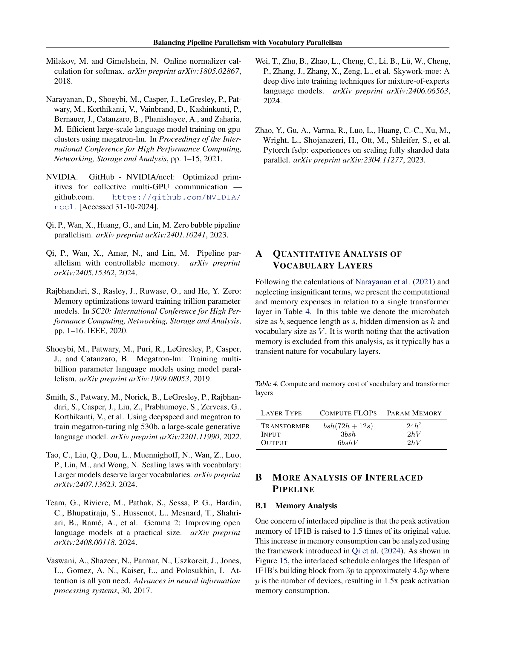
| Layer Type | Compute FLOPs | Param Memory |
|---|---|---|
| Transformer | bsh(72h+12s) | 24h2 |
| Input | 3bsh | 2hV |
| Output | 6bshV | 2hV |
🔼 This table presents a quantitative analysis of the computational and memory costs associated with vocabulary layers compared to transformer layers in large language models. It breaks down the FLOPs (floating-point operations) for computation and the memory usage for parameters in each layer type, providing insights into the computational and memory efficiency of different components within these models.
read the caption
Table 4: Compute and memory cost of vocabulary and transformer layers
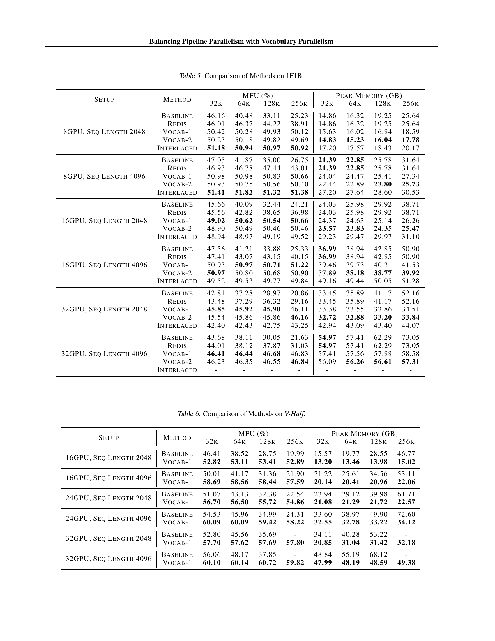
| Setup | Method | MFU (%) 32k | MFU (%) 64k | MFU (%) 128k | MFU (%) 256k | Peak Memory (GB) 32k | Peak Memory (GB) 64k | Peak Memory (GB) 128k | Peak Memory (GB) 256k |
|---|---|---|---|---|---|---|---|---|---|
| 8GPU, Seq Length 2048 | Baseline | 46.16 | 40.48 | 33.11 | 25.23 | 14.86 | 16.32 | 19.25 | 25.64 |
| 8GPU, Seq Length 2048 | Redis | 46.01 | 46.37 | 44.22 | 38.91 | 14.86 | 16.32 | 19.25 | 25.64 |
| 8GPU, Seq Length 2048 | Vocab-1 | 50.42 | 50.28 | 49.93 | 50.12 | 15.63 | 16.02 | 16.84 | 18.59 |
| 8GPU, Seq Length 2048 | Vocab-2 | 50.23 | 50.18 | 49.82 | 49.69 | 14.83 | 15.23 | 16.04 | 17.78 |
| 8GPU, Seq Length 2048 | Interlaced | 51.18 | 50.94 | 50.97 | 50.92 | 17.20 | 17.57 | 18.43 | 20.17 |
| 8GPU, Seq Length 4096 | Baseline | 47.05 | 41.87 | 35.00 | 26.75 | 21.39 | 22.85 | 25.78 | 31.64 |
| 8GPU, Seq Length 4096 | Redis | 46.93 | 46.78 | 47.44 | 43.01 | 21.39 | 22.85 | 25.78 | 31.64 |
| 8GPU, Seq Length 4096 | Vocab-1 | 50.98 | 50.98 | 50.83 | 50.66 | 24.04 | 24.47 | 25.41 | 27.34 |
| 8GPU, Seq Length 4096 | Vocab-2 | 50.93 | 50.75 | 50.56 | 50.40 | 22.44 | 22.89 | 23.80 | 25.73 |
| 8GPU, Seq Length 4096 | Interlaced | 51.41 | 51.82 | 51.32 | 51.38 | 27.20 | 27.64 | 28.60 | 30.53 |
| 16GPU, Seq Length 2048 | Baseline | 45.66 | 40.09 | 32.44 | 24.21 | 24.03 | 25.98 | 29.92 | 38.71 |
| 16GPU, Seq Length 2048 | Redis | 45.56 | 42.82 | 38.65 | 36.98 | 24.03 | 25.98 | 29.92 | 38.71 |
| 16GPU, Seq Length 2048 | Vocab-1 | 49.02 | 50.62 | 50.54 | 50.66 | 24.37 | 24.63 | 25.14 | 26.26 |
| 16GPU, Seq Length 2048 | Vocab-2 | 48.90 | 50.49 | 50.46 | 50.46 | 23.57 | 23.83 | 24.35 | 25.47 |
| 16GPU, Seq Length 2048 | Interlaced | 48.94 | 48.97 | 49.19 | 49.52 | 29.23 | 29.47 | 29.97 | 31.10 |
| 16GPU, Seq Length 4096 | Baseline | 47.56 | 41.21 | 33.88 | 25.33 | 36.99 | 38.94 | 42.85 | 50.90 |
| 16GPU, Seq Length 4096 | Redis | 47.41 | 43.07 | 43.15 | 40.15 | 36.99 | 38.94 | 42.85 | 50.90 |
| 16GPU, Seq Length 4096 | Vocab-1 | 50.93 | 50.97 | 50.71 | 51.22 | 39.46 | 39.73 | 40.31 | 41.53 |
| 16GPU, Seq Length 4096 | Vocab-2 | 50.97 | 50.80 | 50.68 | 50.90 | 37.89 | 38.18 | 38.77 | 39.92 |
| 16GPU, Seq Length 4096 | Interlaced | 49.52 | 49.53 | 49.77 | 49.84 | 49.16 | 49.44 | 50.05 | 51.28 |
| 32GPU, Seq Length 2048 | Baseline | 42.81 | 37.28 | 28.97 | 20.86 | 33.45 | 35.89 | 41.17 | 52.16 |
| 32GPU, Seq Length 2048 | Redis | 43.48 | 37.29 | 36.32 | 29.16 | 33.45 | 35.89 | 41.17 | 52.16 |
| 32GPU, Seq Length 2048 | Vocab-1 | 45.85 | 45.92 | 45.90 | 46.11 | 33.38 | 33.55 | 33.86 | 34.51 |
| 32GPU, Seq Length 2048 | Vocab-2 | 45.54 | 45.86 | 45.86 | 46.16 | 32.72 | 32.88 | 33.20 | 33.84 |
| 32GPU, Seq Length 2048 | Interlaced | 42.40 | 42.43 | 42.75 | 43.25 | 42.94 | 43.09 | 43.40 | 44.07 |
| 32GPU, Seq Length 4096 | Baseline | 43.68 | 38.11 | 30.05 | 21.63 | 54.97 | 57.41 | 62.29 | 73.05 |
| 32GPU, Seq Length 4096 | Redis | 44.01 | 38.12 | 37.87 | 31.03 | 54.97 | 57.41 | 62.29 | 73.05 |
| 32GPU, Seq Length 4096 | Vocab-1 | 46.41 | 46.44 | 46.68 | 46.83 | 57.41 | 57.56 | 57.88 | 58.58 |
| 32GPU, Seq Length 4096 | Vocab-2 | 46.23 | 46.35 | 46.55 | 46.84 | 56.09 | 56.26 | 56.61 | 57.31 |
| 32GPU, Seq Length 4096 | Interlaced | - | - | - | - | - | - | - | - |
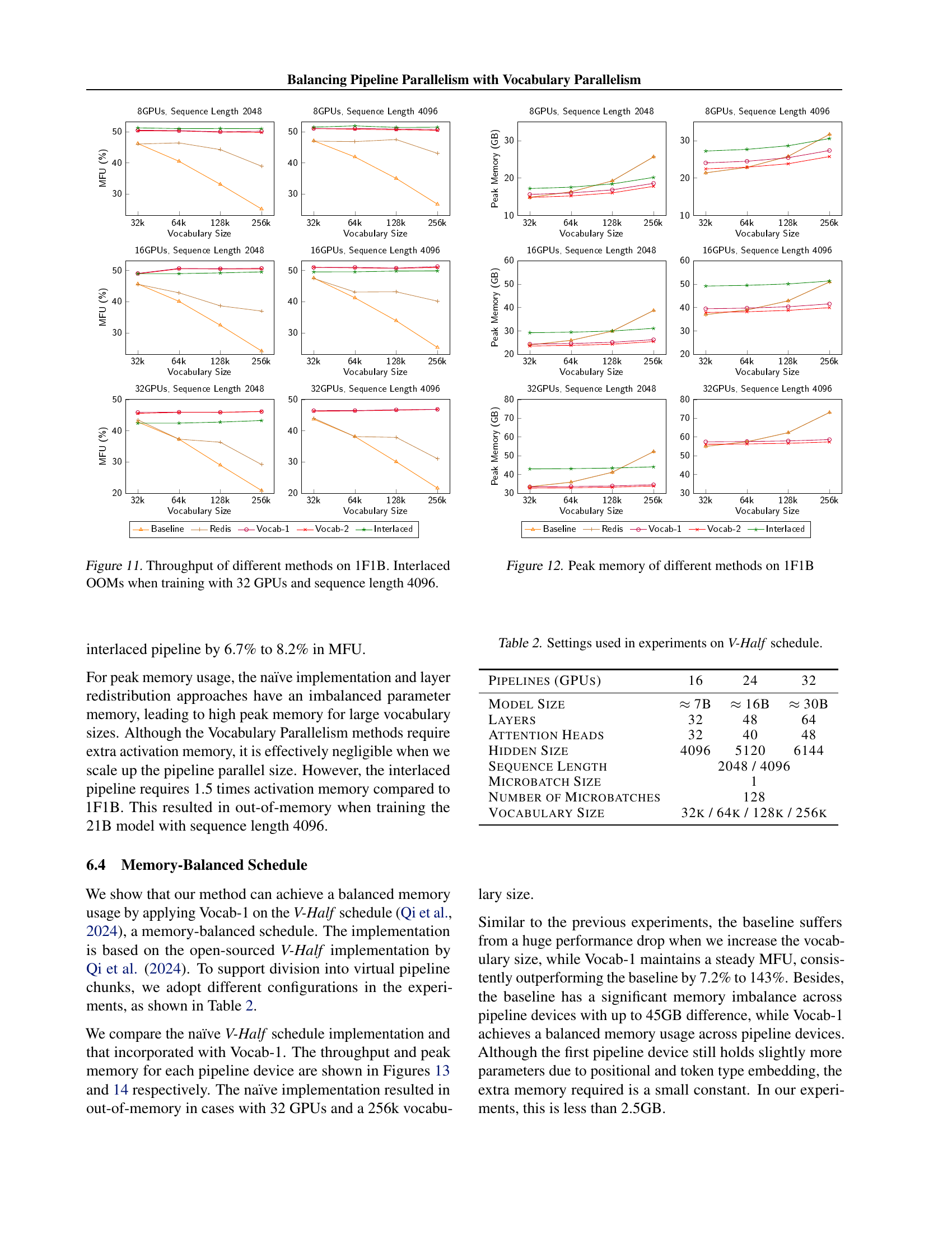
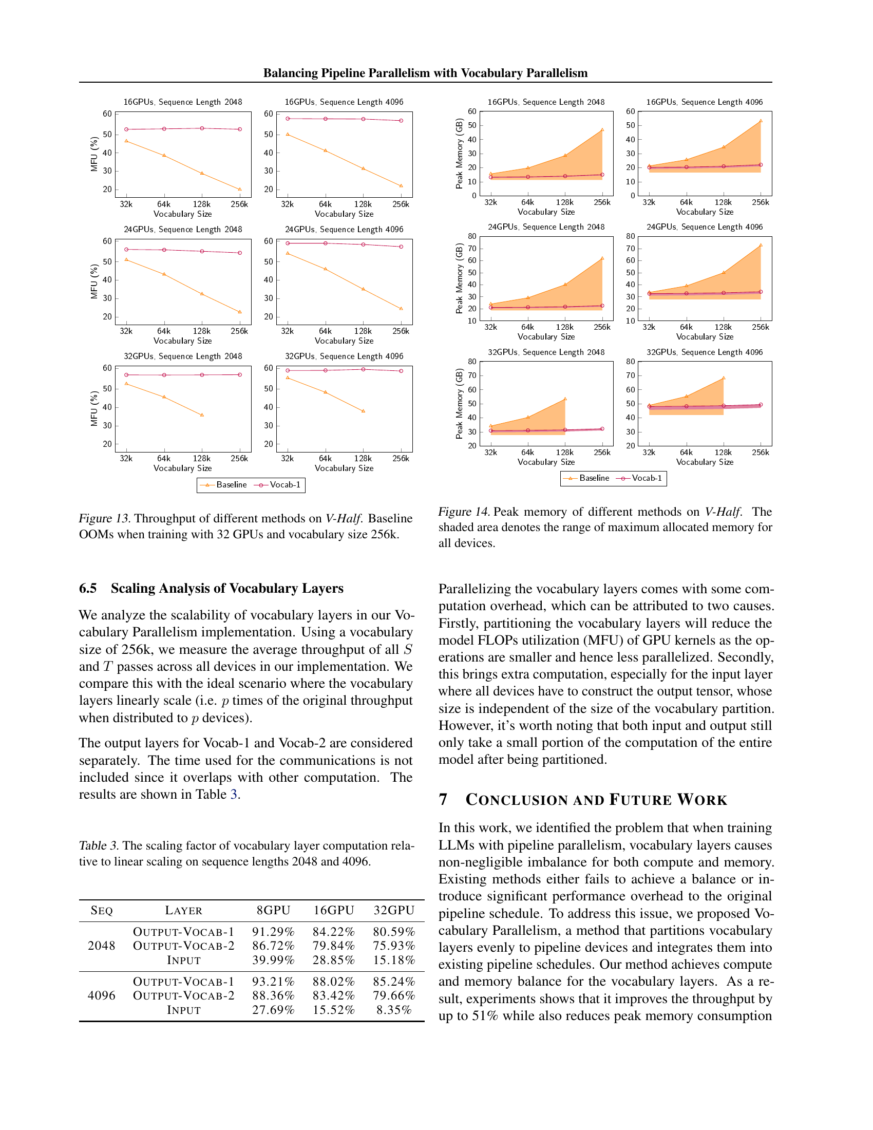
🔼 This table presents a comparison of different methods for training large language models using the 1F1B pipeline parallelism schedule. The methods compared include a baseline approach, a layer redistribution technique, two versions of the proposed Vocabulary Parallelism method (Vocab-1 and Vocab-2), and an interlaced pipeline method. For several model sizes and varying numbers of GPUs, the table shows the achieved model FLOPs utilization (MFU) and peak memory usage for each method. This allows for a quantitative assessment of the effectiveness of each method in improving training throughput and memory efficiency.
read the caption
Table 5: Comparison of Methods on 1F1B.
| Setup | Method | MFU (%) 32k | MFU (%) 64k | MFU (%) 128k | MFU (%) 256k | Peak Memory (GB) 32k | Peak Memory (GB) 64k | Peak Memory (GB) 128k | Peak Memory (GB) 256k |
|---|---|---|---|---|---|---|---|---|---|
| 16GPU, Seq Length 2048 | Baseline | 46.41 | 38.52 | 28.75 | 19.99 | 15.57 | 19.77 | 28.55 | 46.77 |
| Vocab-1 | 52.82 | 53.11 | 53.41 | 52.89 | 13.20 | 13.46 | 13.98 | 15.02 | |
| 16GPU, Seq Length 4096 | Baseline | 50.01 | 41.17 | 31.36 | 21.90 | 21.22 | 25.61 | 34.56 | 53.11 |
| Vocab-1 | 58.69 | 58.56 | 58.44 | 57.59 | 20.14 | 20.41 | 20.96 | 22.06 | |
| 24GPU, Seq Length 2048 | Baseline | 51.07 | 43.13 | 32.38 | 22.54 | 23.94 | 29.12 | 39.98 | 61.71 |
| Vocab-1 | 56.70 | 56.50 | 55.72 | 54.86 | 21.08 | 21.29 | 21.72 | 22.57 | |
| 24GPU, Seq Length 4096 | Baseline | 54.53 | 45.96 | 34.99 | 24.31 | 33.60 | 38.97 | 49.90 | 72.60 |
| Vocab-1 | 60.09 | 60.09 | 59.42 | 58.22 | 32.55 | 32.78 | 33.22 | 34.12 | |
| 32GPU, Seq Length 2048 | Baseline | 52.80 | 45.56 | 35.69 | - | 34.11 | 40.28 | 53.22 | - |
| Vocab-1 | 57.70 | 57.62 | 57.69 | 57.80 | 30.85 | 31.04 | 31.42 | 32.18 | |
| 32GPU, Seq Length 4096 | Baseline | 56.06 | 48.17 | 37.85 | - | 48.84 | 55.19 | 68.12 | - |
| Vocab-1 | 60.10 | 60.14 | 60.72 | 59.82 | 47.99 | 48.19 | 48.59 | 49.38 |
🔼 This table presents a comparison of different methods’ performance on the V-Half pipeline scheduling algorithm. It shows the achieved FLOPs utilization (MFU) and peak memory usage for various model sizes and vocabulary sizes across different numbers of GPUs. The methods compared include the baseline (naive) approach and the proposed Vocabulary Parallelism (Vocab-1) method. The table helps to demonstrate the effectiveness of Vocabulary Parallelism in improving throughput and reducing memory consumption, especially for larger models and vocabularies.
read the caption
Table 6: Comparison of Methods on V-Half.
Full paper#
