↗ arXiv ↗ Hugging Face ↗ Papers with Code
TL;DR#
Large Language Models (LLMs) often struggle with reasoning tasks, relying on greedy decoding or low-temperature sampling which limits diversity and accuracy. Existing sampling methods like top-k, top-p, and nucleus sampling don’t effectively filter noise, creating a trade-off between accuracy and variety. High temperatures exacerbate this issue by introducing even more noise.
This paper introduces top-ησ, a novel sampling method addressing these limitations. Top-ησ operates directly on pre-softmax logits, identifying a statistical threshold to separate informative tokens from noise. It maintains sampling space stability regardless of temperature, unlike other methods. Extensive experiments demonstrate that top-ησ consistently outperforms existing techniques and greedy decoding, even at high temperatures, and improves generation quality on multiple reasoning-focused datasets.
Key Takeaways#
Why does it matter?#
This paper is important because it challenges conventional wisdom in large language model (LLM) decoding by introducing a novel sampling method, top-ησ. Top-ησ outperforms existing methods and even surpasses greedy decoding, opening new avenues for improving LLM reasoning capabilities and test-time scaling techniques. Its theoretical analysis and empirical validation on diverse datasets provide strong support and offer valuable insights for researchers. This research is highly relevant to the current focus on enhancing LLM reasoning and efficiency, particularly in light of the rising interest in test-time scaling.
Visual Insights#

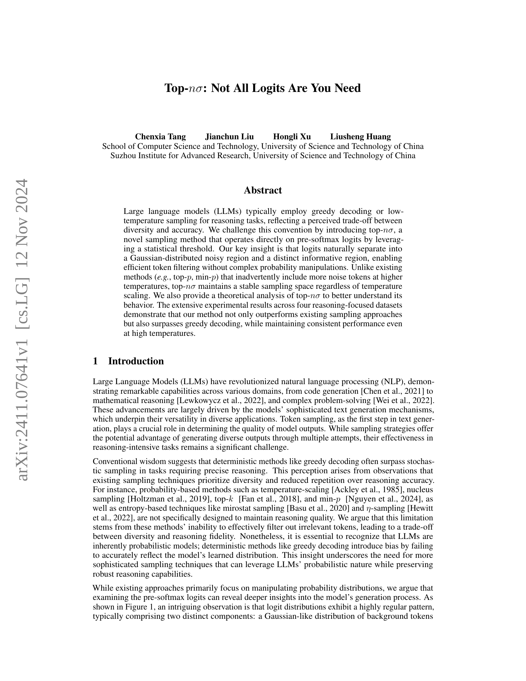
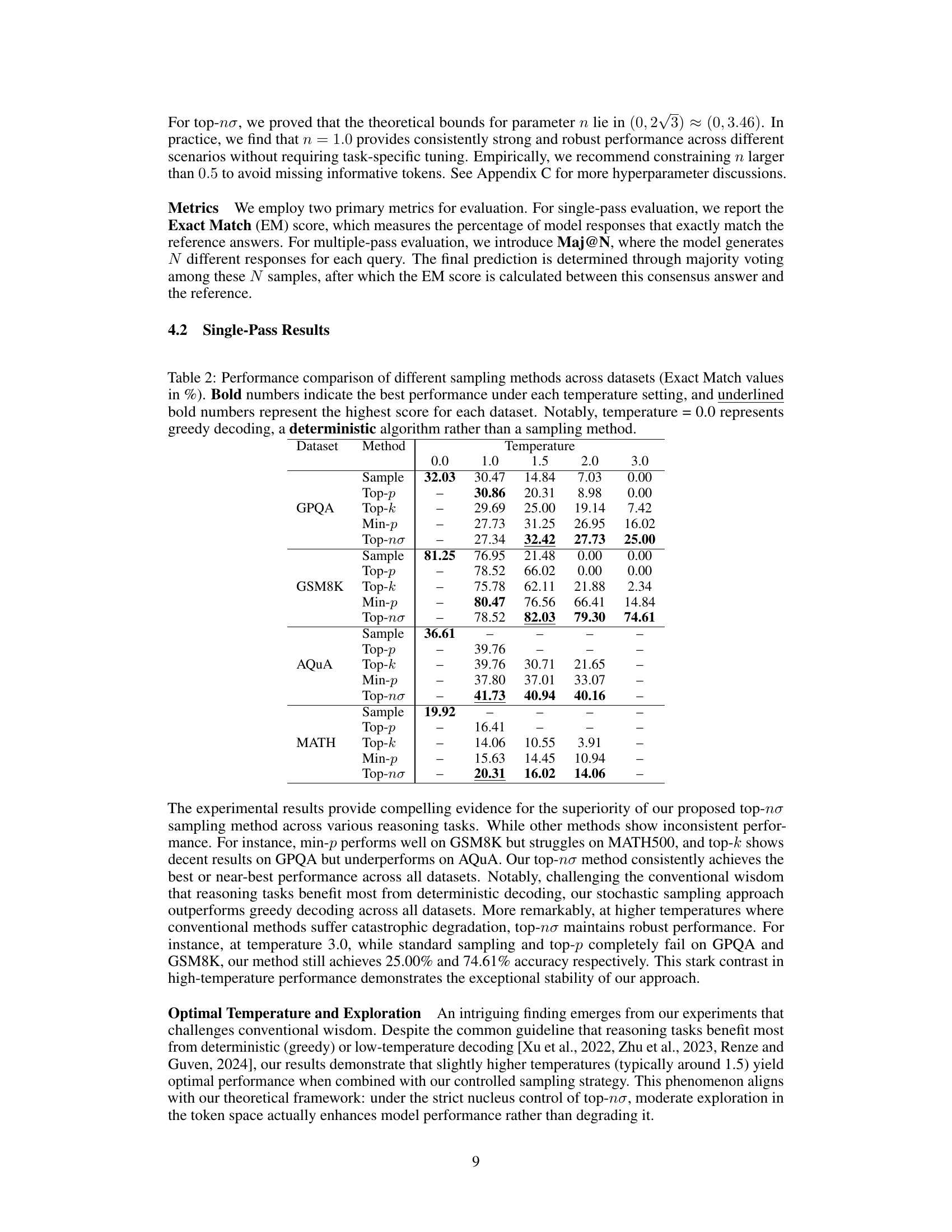
🔼 The figure shows the distribution of pre-softmax logits from the LLaMA3-8B-Instruct model on an AQUA dataset sample. The left panel (a) presents a histogram of the logits, revealing a distinct bimodal distribution. A large portion of logits cluster around a central mean, resembling a Gaussian distribution, representing ’noise’. A smaller, but more significant number of tokens have substantially larger logit values forming the ‘informative’ region, which is separate from the noise. The right panel (b) displays the token probabilities (post-softmax) sorted in descending order. It visually emphasizes how the few tokens with the largest logits contribute most of the probability mass. This illustrates that the informative tokens are easily distinguishable from the noise tokens by looking at the logits.
read the caption
(a) Distribution of logits
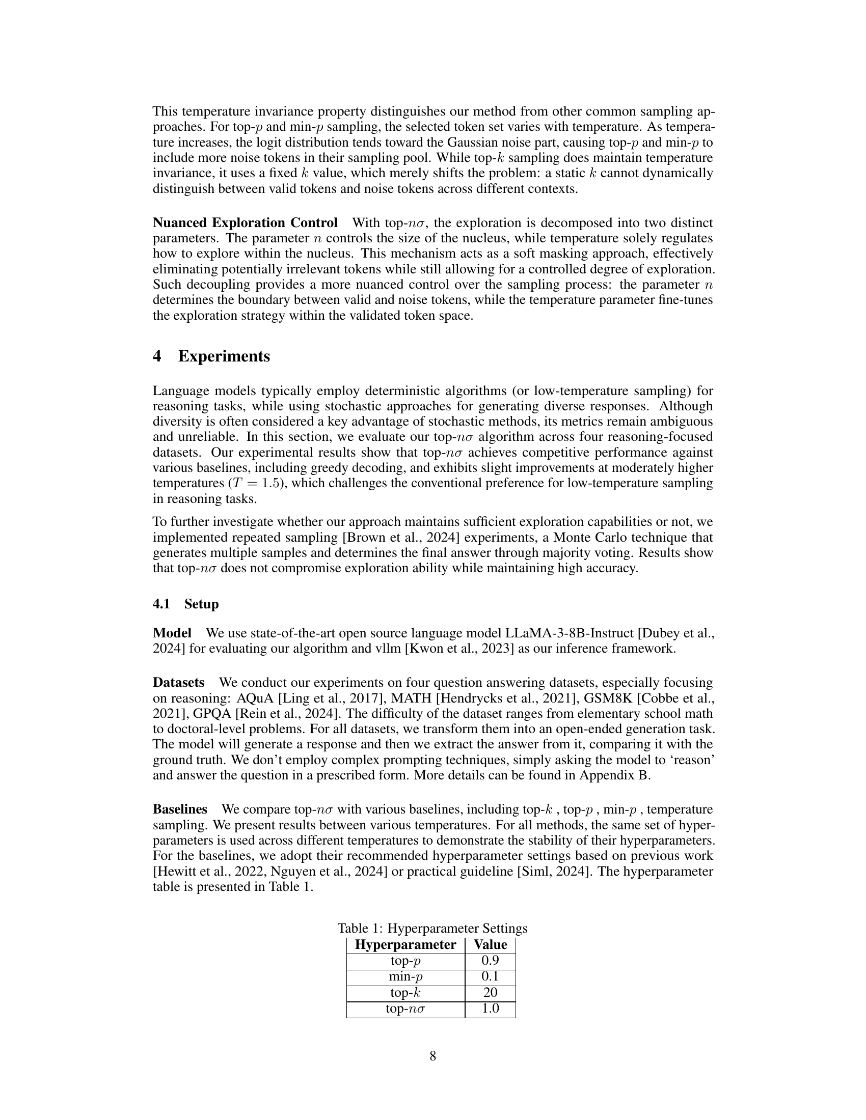
| Hyperparameter | Value |
|---|---|
| top-$p$ | 0.9 |
| min-$p$ | 0.1 |
| top-$k$ | 20 |
| top-$n\sigma$ | 1.0 |
🔼 This table shows the hyperparameter settings used for different sampling methods in the experiments. It lists the hyperparameters used for Top-p, Min-p, Top-k, and the proposed Top-ησ sampling methods. The values chosen for these hyperparameters reflect those recommended in prior work or common practices for these methods. This ensures a fair comparison between the proposed Top-ησ method and existing baselines.
read the caption
Table 1: Hyperparameter Settings
In-depth insights#
Logit Space Analysis#
A Logit Space Analysis of large language models (LLMs) would offer crucial insights into their inner workings. By directly examining pre-softmax logits, rather than post-softmax probabilities, we can gain a deeper understanding of the model’s reasoning process. This approach allows us to move beyond probability-based sampling methods, like top-k or nucleus sampling, and potentially discover more efficient and effective sampling strategies. A key aspect of such an analysis would involve characterizing the distribution of logits, potentially identifying distinct regions like a Gaussian-distributed ’noise’ region and an ‘informative’ region containing the most relevant tokens. Understanding the interplay between these regions at different temperatures is critical. The analysis could reveal how to optimally filter out noise tokens, leading to improved reasoning capabilities while retaining desirable diversity. Finally, a logit-based perspective may also offer valuable insights for model training and architecture optimization, potentially by informing strategies to reduce the magnitude of the noise region during model training, which would translate into improved performance during inference.
Top-ησ Algorithm#
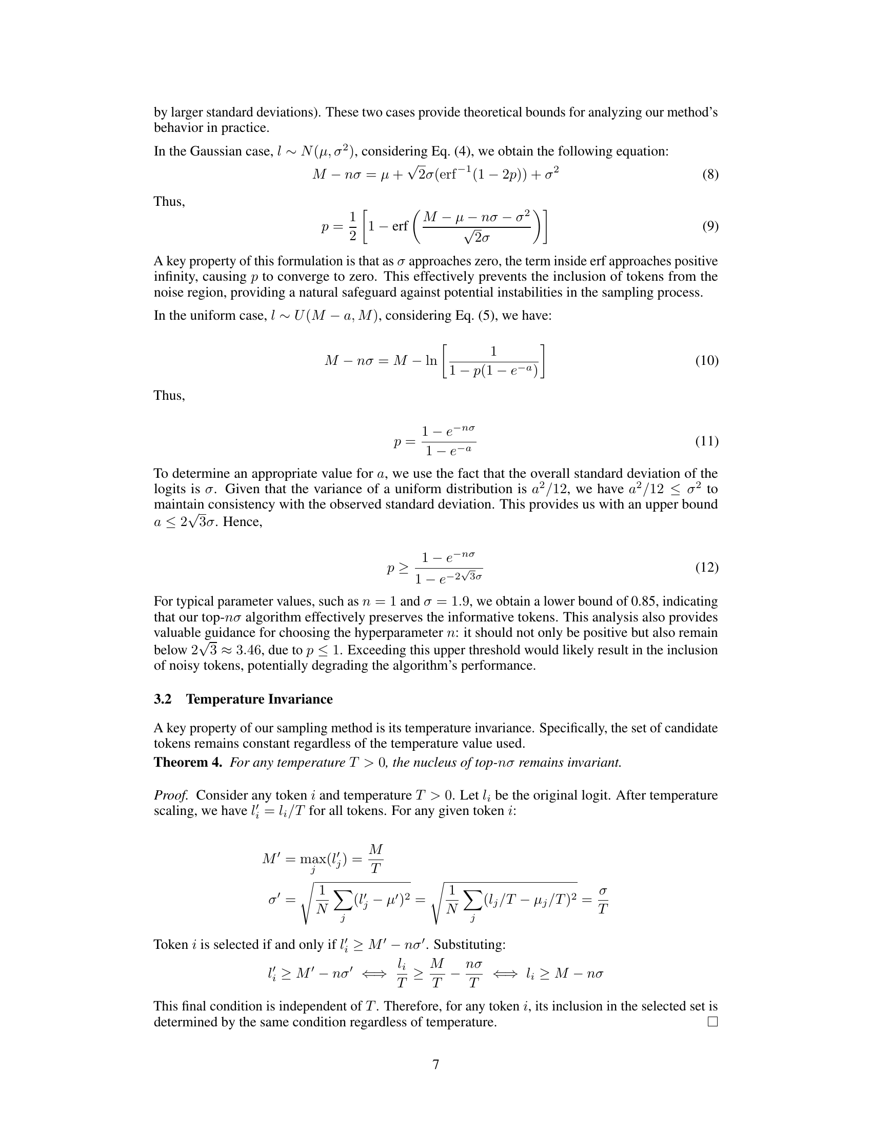
The proposed Top-ησ algorithm offers a novel approach to token sampling in large language models (LLMs). Instead of manipulating probability distributions directly (like top-p or nucleus sampling), it operates on pre-softmax logits, identifying a distinct informative region separate from a Gaussian-distributed noise region. This is achieved by using a statistical threshold based on the maximum logit and the standard deviation, effectively filtering out noisy tokens without complex probability calculations or sorting. A key advantage is its temperature invariance: the sampling space remains stable regardless of temperature scaling, unlike other methods that become increasingly noisy at higher temperatures. This robustness makes it particularly suitable for test-time scaling techniques that rely on extensive sampling. Furthermore, its simplicity and computational efficiency are noteworthy, operating directly on logits without requiring additional softmax transformations. The algorithm’s effectiveness is demonstrated empirically across various datasets, outperforming existing sampling methods and even greedy decoding. The theoretical analysis provides a solid foundation, analyzing its behavior under Gaussian and uniform logit distributions, establishing theoretical bounds and proving temperature invariance. Its ability to balance exploration and exploitation is also significant, separating control over nucleus size from temperature control.
Temp. Invariance Proof#
The temperature invariance proof is a crucial component of the research paper, demonstrating a key advantage of the proposed top-ησ sampling method. It rigorously shows that the set of selected tokens remains consistent regardless of the temperature parameter used during sampling. This temperature invariance is a significant departure from existing sampling methods like top-p and min-p, which exhibit varying token selection as temperature changes. The proof’s significance lies in ensuring the stability and reliability of top-ησ, preventing the inclusion of noisy tokens that may negatively impact performance at higher temperatures. The underlying mathematical derivation provides strong theoretical support for the algorithm’s robustness, which is further validated by the experimental results, showcasing consistent performance even in high-temperature settings. This robustness and stability are critical for applying the sampling method in situations where extensive sampling or test-time scaling techniques are necessary, thereby highlighting a key strength of top-ησ over existing methods.
Reasoning Datasets#
A dedicated section on “Reasoning Datasets” in a research paper would be crucial for evaluating the performance of large language models (LLMs) on tasks requiring logical deduction and inference. The choice of datasets is critical; they should represent a diverse range of reasoning challenges, reflecting varying levels of difficulty and complexity. Ideally, the datasets would be carefully curated to minimize biases and ensure that the evaluation fairly assesses an LLM’s reasoning capabilities. The inclusion of benchmark datasets, widely accepted in the field, would enable comparison with existing state-of-the-art models, thus providing a strong basis for performance analysis. Furthermore, a detailed description of the datasets, including their size, the nature of reasoning tasks presented, and the characteristics of the questions posed, would enhance the transparency and reproducibility of the research. Beyond established benchmarks, including newly developed or lesser-known datasets could reveal interesting aspects of LLM reasoning performance. A careful selection of both standard and novel datasets would paint a more complete picture of an LLM’s strengths and weaknesses in reasoning. This comprehensive approach ensures that the research is not only rigorous and verifiable but also advances the broader understanding of LLMs’ capabilities and limitations in performing logical reasoning.
Future Work#
The paper’s conclusion points towards promising avenues for future research. Investigating the interplay between the training data’s inherent noise and the resulting Gaussian distribution in logits is crucial. A deeper understanding could lead to improved training techniques that directly address the noise issue, potentially enhancing model performance and generalization. Furthermore, exploring how to leverage the identified properties of logit distributions during the training process itself warrants further study. This might involve developing new model architectures or training strategies that explicitly address the separation between informative and noisy regions. This targeted approach could result in more efficient and robust models. Finally, extending the top-ησ method to other test-time scaling techniques beyond repeated sampling is essential. Exploring how this approach could improve performance when coupled with techniques such as test-time augmentation or multi-sampling would provide valuable insights, and potentially lead to significant advancements in LLM capabilities.
More visual insights#
More on figures

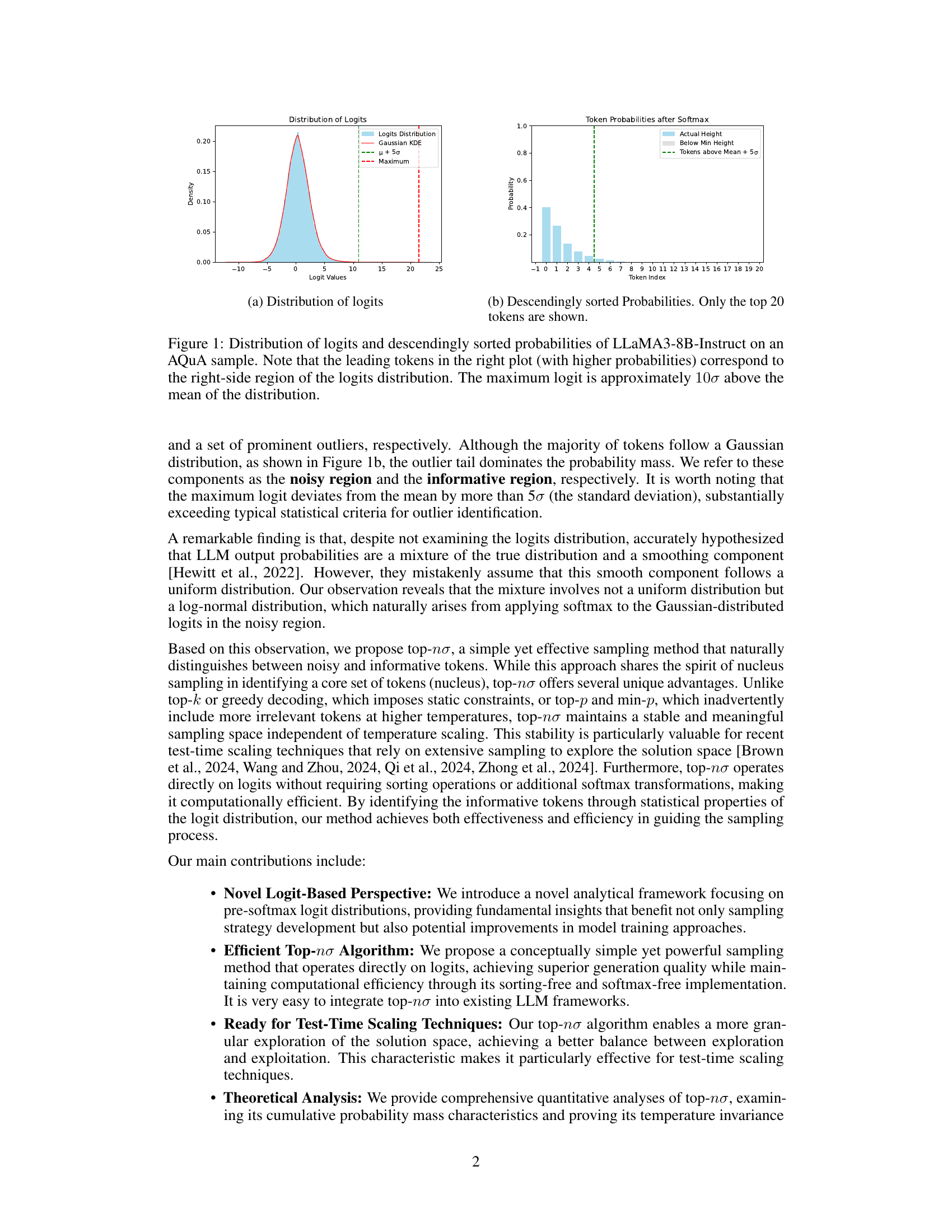
🔼 This figure’s (b) part shows the probabilities of the top 20 tokens after applying the softmax function to the logits. It visually demonstrates how a small number of tokens (the most likely ones) account for the majority of the probability mass, while the vast majority of tokens have very low probabilities. This highlights the key concept of the paper: that logits naturally separate into a Gaussian-distributed noisy region and a distinct informative region, with the informative tokens having much higher logits.
read the caption
(b) Descendingly sorted Probabilities. Only the top 20 tokens are shown.

🔼 This figure visualizes the distribution of pre-softmax logits and the resulting probabilities after applying the softmax function for a single sample from the AQuA dataset using the LLaMA3-8B-Instruct language model. The left panel (a) shows a histogram of the logits, highlighting their approximately Gaussian distribution with a significant outlier tail. A Kernel Density Estimate (KDE) curve is overlaid to emphasize the Gaussian component. The right panel (b) displays the probabilities of the top 20 tokens in descending order. The key observation is the strong correspondence between the tokens with the highest probabilities (on the right of plot (b)) and the high-logit outliers in the right tail of the logit distribution (on the right of plot (a)). The maximum logit is considerably larger than the mean of the distribution (approximately 10 standard deviations greater), clearly distinguishing a small number of ‘informative’ tokens from the bulk of ’noisy’ tokens.
read the caption
Figure 1: Distribution of logits and descendingly sorted probabilities of LLaMA3-8B-Instruct on an AQuA sample. Note that the leading tokens in the right plot (with higher probabilities) correspond to the right-side region of the logits distribution. The maximum logit is approximately 10σ10𝜎10\sigma10 italic_σ above the mean of the distribution.

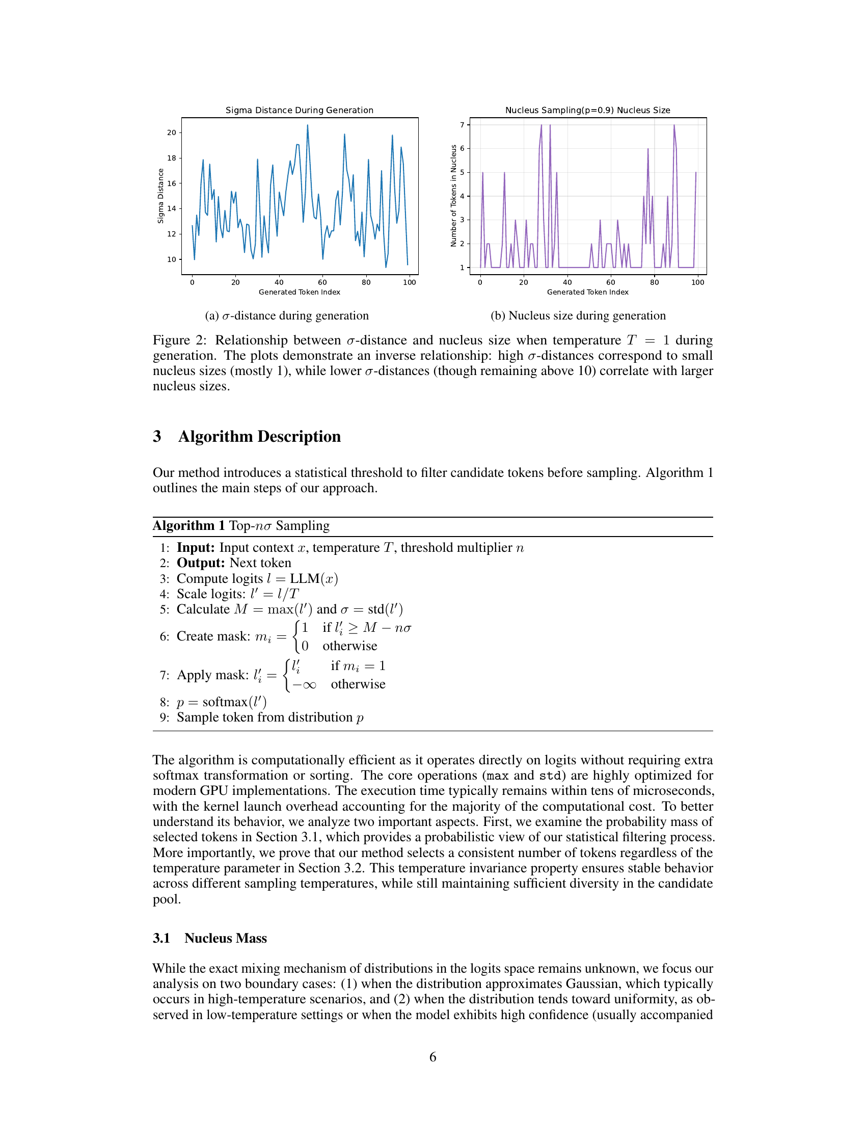
🔼 The figure shows the σ-distance, which is the number of standard deviations between the maximum probability and the mean value of the logit distribution, over the course of text generation. It visually represents how much the maximum logit value deviates from the average logit values throughout the generation process. This metric is used to assess the model’s confidence at different generation stages. A higher σ-distance implies higher confidence because the maximum logit is significantly above the average, and a lower σ-distance suggests less certainty.
read the caption
(a) σ𝜎\sigmaitalic_σ-distance during generation
More on tables
| Dataset | Method | 0.0 | 1.0 | 1.5 | 2.0 | 3.0 |
|---|---|---|---|---|---|---|
| GPQA | Sample | 32.03 | 30.47 | 14.84 | 7.03 | 0.00 |
| Top-p | 30.86 | 20.31 | 8.98 | 0.00 | ||
| Top-k | 29.69 | 25.00 | 19.14 | 7.42 | ||
| Min-p | 27.73 | 31.25 | 26.95 | 16.02 | ||
| Top-nσ | 27.34 | 32.42 | 27.73 | 25.00 | ||
| GSM8K | Sample | 81.25 | 76.95 | 21.48 | 0.00 | 0.00 |
| Top-p | 78.52 | 66.02 | 0.00 | 0.00 | ||
| Top-k | 75.78 | 62.11 | 21.88 | 2.34 | ||
| Min-p | 80.47 | 76.56 | 66.41 | 14.84 | ||
| Top-nσ | 78.52 | 82.03 | 79.30 | 74.61 | ||
| AQuA | Sample | 36.61 | – | – | – | – |
| Top-p | 39.76 | – | – | – | – | |
| Top-k | 39.76 | 30.71 | 21.65 | – | – | |
| Min-p | 37.80 | 37.01 | 33.07 | – | – | |
| Top-nσ | 41.73 | 40.94 | 40.16 | – | – | |
| MATH | Sample | 19.92 | – | – | – | – |
| Top-p | 16.41 | – | – | – | – | |
| Top-k | 14.06 | 10.55 | 3.91 | – | – | |
| Min-p | 15.63 | 14.45 | 10.94 | – | – | |
| Top-nσ | 20.31 | 16.02 | 14.06 | – | – |
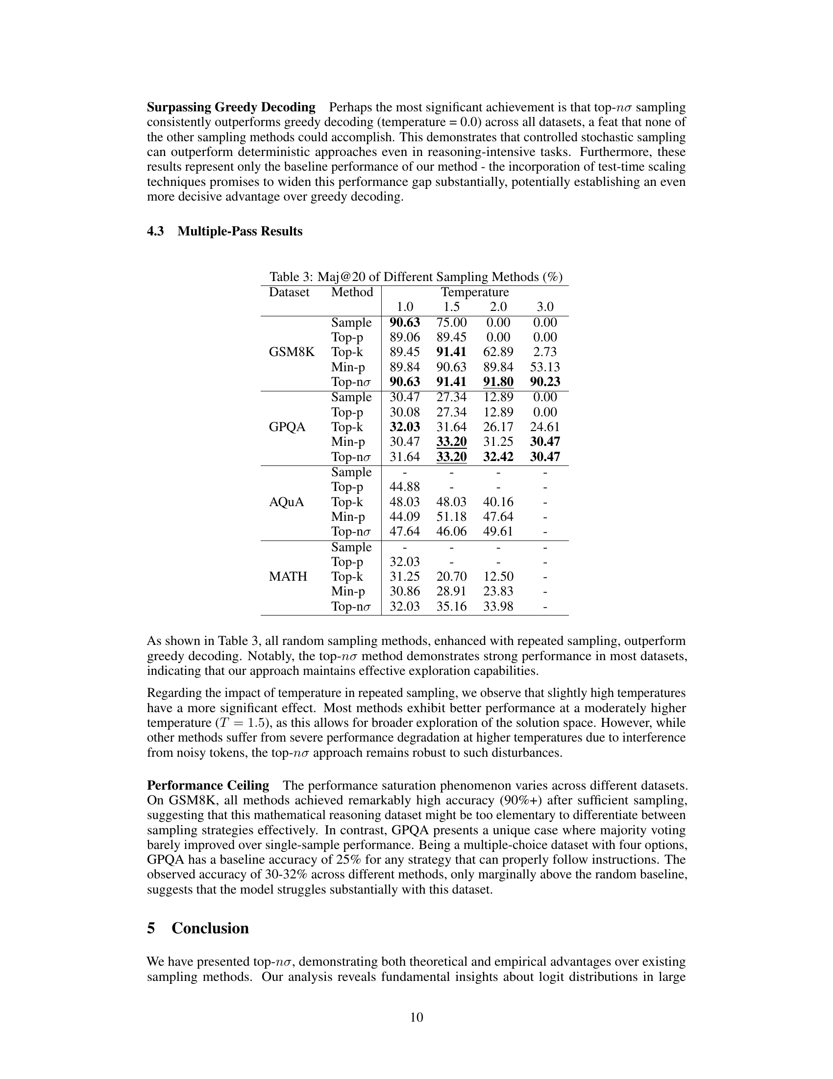
🔼 Table 2 presents a comprehensive comparison of different sampling methods’ performance across four datasets, focusing on the Exact Match (EM) metric. The EM score indicates the percentage of perfectly correct answers generated by each method. The table compares results across various temperatures (0.0, 1.0, 1.5, 2.0, 3.0). A temperature of 0.0 represents greedy decoding, a deterministic approach, while other temperatures indicate different levels of stochasticity in the sampling process. The best performance under each temperature setting is highlighted in bold, and the overall best performance for each dataset is additionally emphasized with an underline. This allows for a direct comparison of the methods’ performance across different datasets and varying degrees of randomness in the generation process.
read the caption
Table 2: Performance comparison of different sampling methods across datasets (Exact Match values in %). Bold numbers indicate the best performance under each temperature setting, and underlined bold numbers represent the highest score for each dataset. Notably, temperature = 0.0 represents greedy decoding, a deterministic algorithm rather than a sampling method.
| Dataset | Method | Temperature | ||||
|---|---|---|---|---|---|---|
| GSM8K | Sample | 90.63 | 75.00 | 0.00 | 0.00 | |
| Top-p | 89.06 | 89.45 | 0.00 | 0.00 | ||
| Top-k | 89.45 | 91.41 | 62.89 | 2.73 | ||
| Min-p | 89.84 | 90.63 | 89.84 | 53.13 | ||
| Top-nσ | 90.63 | 91.41 | 91.80 | 90.23 | ||
| GPQA | Sample | 30.47 | 27.34 | 12.89 | 0.00 | |
| Top-p | 30.08 | 27.34 | 12.89 | 0.00 | ||
| Top-k | 32.03 | 31.64 | 26.17 | 24.61 | ||
| Min-p | 30.47 | 33.20 | 31.25 | 30.47 | ||
| Top-nσ | 31.64 | 33.20 | 32.42 | 30.47 | ||
| AQuA | Sample | - | - | - | - | |
| Top-p | 44.88 | - | - | - | ||
| Top-k | 48.03 | 48.03 | 40.16 | - | ||
| Min-p | 44.09 | 51.18 | 47.64 | - | ||
| Top-nσ | 47.64 | 46.06 | 49.61 | - | ||
| MATH | Sample | - | - | - | - | |
| Top-p | 32.03 | - | - | - | ||
| Top-k | 31.25 | 20.70 | 12.50 | - | ||
| Min-p | 30.86 | 28.91 | 23.83 | - | ||
| Top-nσ | 32.03 | 35.16 | 33.98 | - |
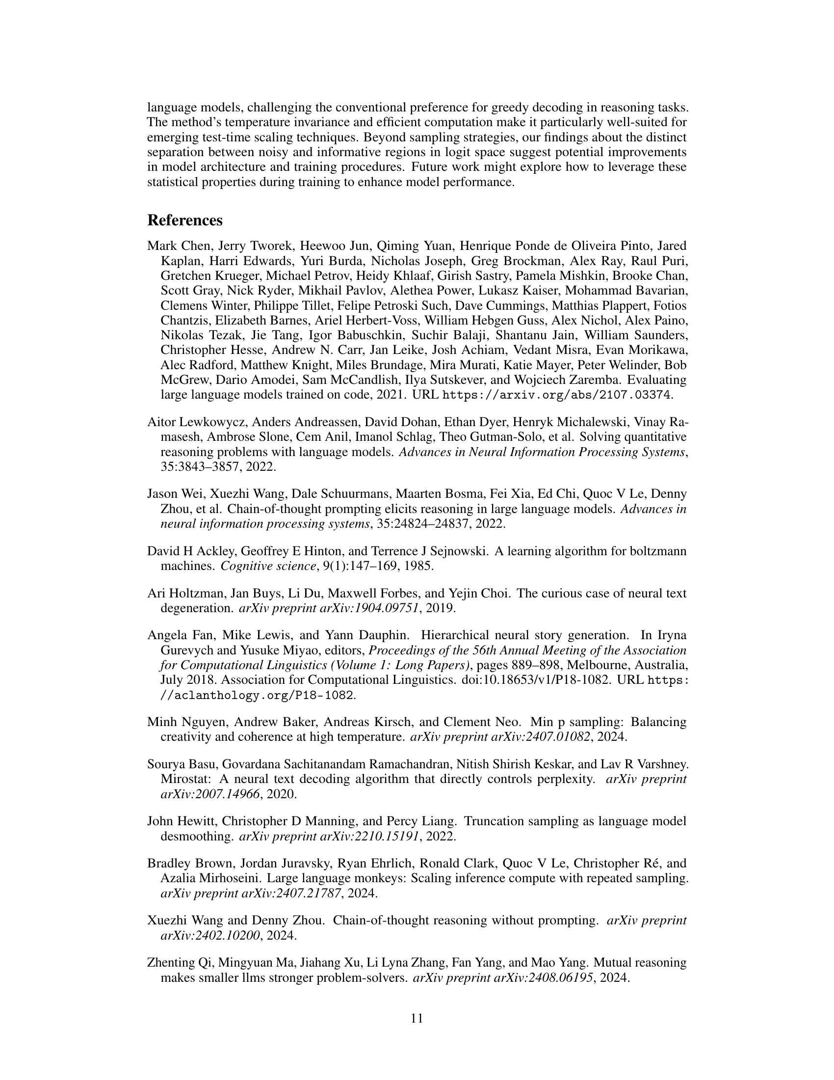
🔼 This table presents the performance of various sampling methods (Sample, Top-p, Top-k, Min-p, and Top-ησ) using the Maj@20 metric, which represents the accuracy of majority voting among 20 model-generated answers. The results are categorized by dataset (GSM8K, GPQA, AQUA, MATH) and temperature setting (1.0, 1.5, 2.0, 3.0), showing how different sampling strategies and temperature values affect the final answer’s accuracy.
read the caption
Table 3: Maj@20 of Different Sampling Methods (%)
Full paper#
