↗ arXiv ↗ Hugging Face ↗ Papers with Code
TL;DR#
Generating high-quality 3D models remains computationally expensive, particularly at high resolutions. Existing methods struggle with representing complex geometries and fine details efficiently, often sacrificing quality for computational feasibility. This results in limitations in generating detailed and diverse 3D shapes, a crucial need for many applications. This paper introduces Wavelet Latent Diffusion (WaLa), a novel approach that addresses these limitations by using wavelet-based, compact latent encodings of 3D shapes. This method efficiently trains a large-scale generative model, achieving a remarkable compression ratio without significant loss of detail.
WaLa, with its approximately one billion parameters, generates high-quality 3D shapes at 2563 resolution. The model’s performance surpasses state-of-the-art results across diverse datasets and input modalities, including text, images, sketches, point clouds, and more. Furthermore, WaLa’s fast inference times (2-4 seconds) make it highly practical for various applications. The model’s impressive performance, along with the open-sourced code and pre-trained models, makes it a significant contribution to the field of 3D generative modeling.
Key Takeaways#
Why does it matter?#
This paper is crucial because it introduces WaLa, a groundbreaking 3D generative model that achieves state-of-the-art results in both quality and speed. Its efficient wavelet-based encoding and billion-parameter scale open exciting avenues for large-scale 3D generation and diverse applications. The open-sourced code and pretrained models significantly benefit the community. The exploration of diverse input modalities is also highly relevant to current trends.
Visual Insights#

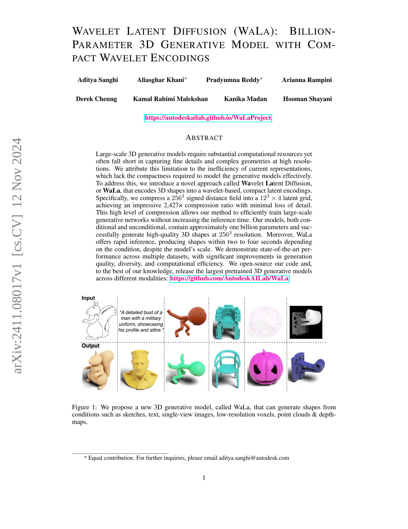
🔼 Figure 1 showcases the capabilities of the Wavelet Latent Diffusion (WaLa) model, a novel 3D generative model. The figure displays example inputs (sketches, text descriptions, single-view images, low-resolution voxel grids, point clouds, and depth maps) and their corresponding generated 3D outputs. This demonstrates the model’s ability to create diverse 3D shapes from various types of input conditions, highlighting its versatility and potential applications.
read the caption
Figure 1: We propose a new 3D generative model, called WaLa, that can generate shapes from conditions such as sketches, text, single-view images, low-resolution voxels, point clouds & depth-maps.
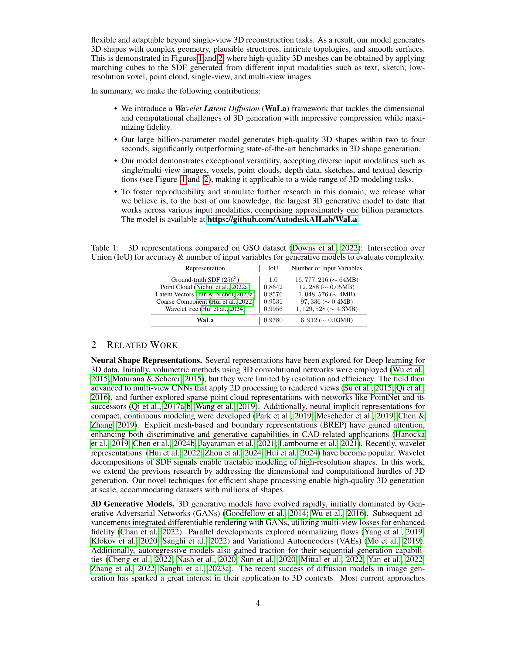
| Representation | IoU | Number of Input Variables |
|---|---|---|
| Ground-truth SDF (2563) | 1.0 | 16,777,216 (~64MB) |
| Point Cloud (Nichol et al., 2022a) | 0.8642 | 12,288 (~0.05MB) |
| Latent Vectors (Jun & Nichol, 2023a) | 0.8576 | 1,048,576 (~4MB) |
| Coarse Component (Hui et al., 2022) | 0.9531 | 97,336 (~0.4MB) |
| Wavelet tree (Hui et al., 2024) | 0.9956 | 1,129,528 (~4.3MB) |
| WaLa | 0.9780 | 6,912 (~0.03MB) |
🔼 This table compares different 3D shape representations used in generative models, focusing on their performance on the GSO dataset and their complexity. It shows the Intersection over Union (IoU) score, which measures the accuracy of the representation, and the number of input variables required for the generative model, which indicates the complexity. By comparing these two metrics, the table helps to understand the trade-offs between accuracy and complexity of various 3D shape representations for large-scale generative modeling.
read the caption
Table 1: 3D representations compared on GSO dataset (Downs et al., 2022): Intersection over Union (IoU) for accuracy & number of input variables for generative models to evaluate complexity.
In-depth insights#
Wavelet Encoding#
Wavelet encoding, in the context of 3D generative models, offers a powerful approach to compress high-dimensional shape representations like signed distance fields (SDFs). Traditional methods often struggle with the cubic complexity of 3D data, leading to computational bottlenecks. Wavelets, however, provide a multi-resolution, hierarchical decomposition that allows for efficient compression by discarding less significant details in higher frequency bands. This compression is crucial for training large-scale generative models, as it significantly reduces the input dimensionality, and thus, the computational resources needed during both training and inference. The inherent multi-resolution nature of wavelets is also beneficial for capturing both fine details and global structures in 3D shapes, which improves the quality and diversity of generated models. However, efficient and effective wavelet encoding for 3D shapes requires careful consideration of the wavelet transform used, the level of compression, and the subsequent reconstruction process to minimize information loss. The choice of wavelet basis and thresholding strategy is vital for optimizing the balance between compression and reconstruction quality. Furthermore, the integration of wavelet encodings within the overall architecture of a generative model needs careful design to leverage the benefits fully and to avoid introducing new challenges.
Diffusion Model#
Diffusion models, a class of generative models, have revolutionized image generation. Their strength lies in their ability to generate high-quality samples by gradually adding noise to data until it becomes pure noise, and then reversing this process to reconstruct the data. This approach avoids the common pitfalls of other generative models like GANs (Generative Adversarial Networks), such as mode collapse and training instability. The process of denoising is learned by a neural network, which is trained on a large dataset. Furthermore, the flexibility of diffusion models allows for easy incorporation of conditioning information such as text prompts, sketches, or other images to control the generation process, making them highly versatile tools in various creative and scientific applications. However, they are computationally expensive, requiring significant memory and processing power, especially for high-resolution outputs. Research continues to address these challenges and optimize these models for broader accessibility.
Multimodal 3D#
Multimodal 3D generation signifies a paradigm shift in 3D modeling, moving beyond single-modality approaches (like only text or images) to leverage the power of multiple input sources simultaneously. This approach is crucial because real-world object understanding often relies on integrating diverse information streams. The challenges inherent in multimodal 3D generation include: handling diverse data formats, aligning modalities effectively, and managing computational complexity. However, the rewards are significant. A successful multimodal system can produce more realistic, detailed, and nuanced 3D models. Key innovations in this field might involve novel architectures combining strengths of different model types (e.g., transformers and diffusion models) or advanced fusion techniques that effectively weigh the relative importance of various input modalities in generating a final 3D output. The potential applications of multimodal 3D are vast, ranging from game development to CAD and medical imaging. Future research directions include improving robustness to noisy or incomplete data and creating systems capable of interactive generation and editing of 3D models based on multimodal feedback.
Ablation Studies#
The ablation study section of a research paper is crucial for understanding the contribution of individual components to the overall performance. In the context of a 3D generative model, an ablation study might systematically remove or alter different parts of the model’s architecture or training process, such as the adaptive sampling loss, VQ-VAE, or the generative model itself. By observing how performance metrics change (e.g., IoU, MSE, LFD) after removing each component, researchers can assess the relative importance of each part and identify potential areas for improvement. A well-designed ablation study should systematically vary each parameter, providing a quantitative understanding of the specific impact of each component. It’s vital to have a control group, maintaining the original model for comparison. For example, removing the adaptive sampling loss might lead to a decrease in IoU, suggesting that this loss is particularly effective in reconstructing fine-grained detail in 3D shapes. Similarly, an ablation study might explore various wavelet transformations or the number of parameters in a diffusion model, showing the optimal configurations for balancing performance and computational cost. The conclusions drawn from an ablation study often dictate future research directions and help to solidify the contributions of the paper.
Future Works#
Future work could explore several promising avenues. Improving the efficiency of the wavelet encoding process is crucial; reducing the computational overhead while preserving detail would significantly enhance scalability. Exploring alternative wavelet transforms beyond biorthogonal wavelets might yield better compression ratios or reconstruction quality. Investigating more sophisticated diffusion model architectures to further enhance generation speed and fidelity is also warranted, potentially including exploring alternative architectures or incorporating attention mechanisms more effectively. Expanding the range of input modalities is vital, with a focus on high-fidelity data sources and more complex interactions between modalities. Finally, thorough investigation into zero-shot generalization capabilities and robustness to noisy or incomplete input data is necessary for broader real-world applications, and a detailed analysis of biases inherent in the dataset and model training is important to ensure fair and equitable outcomes.
More visual insights#
More on figures

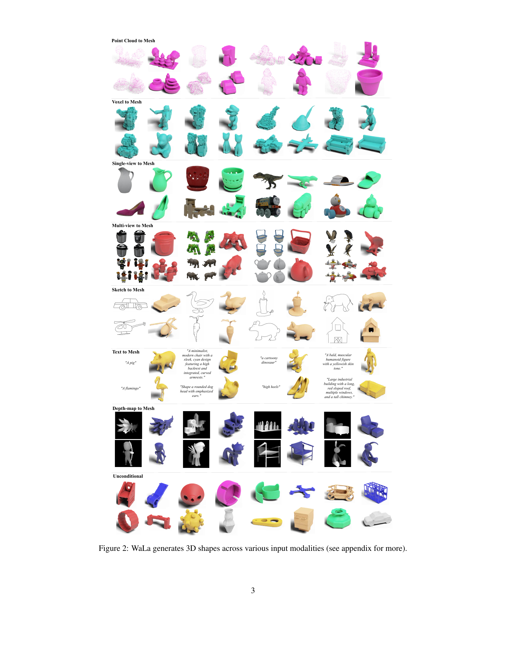
🔼 Figure 2 showcases the versatility of the WaLa model by demonstrating its ability to generate a wide variety of 3D shapes from different input types. These inputs include point clouds, voxels, single-view images, multi-view images, sketches, and text descriptions. The figure displays several example outputs for each input modality, highlighting the model’s capacity to create high-quality, detailed, and diverse 3D shapes across multiple representations and conditions. More examples are available in the paper’s appendix.
read the caption
Figure 2: WaLa generates 3D shapes across various input modalities (see appendix for more).

🔼 Figure 3 illustrates the WaLa model’s architecture and workflow. The top-left panel depicts Stage 1 training, where a VQ-VAE autoencoder compresses a high-resolution wavelet tree representation of a 3D shape (W) into a lower-dimensional latent space (Z). The top-right panel shows Stage 2, the conditional/unconditional diffusion training process on the latent representations to generate new shapes. The bottom panel details the inference process: starting with random noise, the diffusion model generates a latent code (Z), which is then decoded into a wavelet tree (W) and finally converted into a mesh representation of the 3D shape.
read the caption
Figure 3: Overview of the WaLa network architecture and 2-stage training process and inference method. Top Left: Stage 1 autoencoder training, compressing diffusible wavelet tree (W𝑊Witalic_W) shape representation into a compact latent space. Top Right: Conditional/unconditional diffusion training. Bottom: Inference pipeline, illustrating sampling from the trained diffusion model and decoding the sampled latent into a Wavelet Tree (W𝑊Witalic_W), then into a mesh.

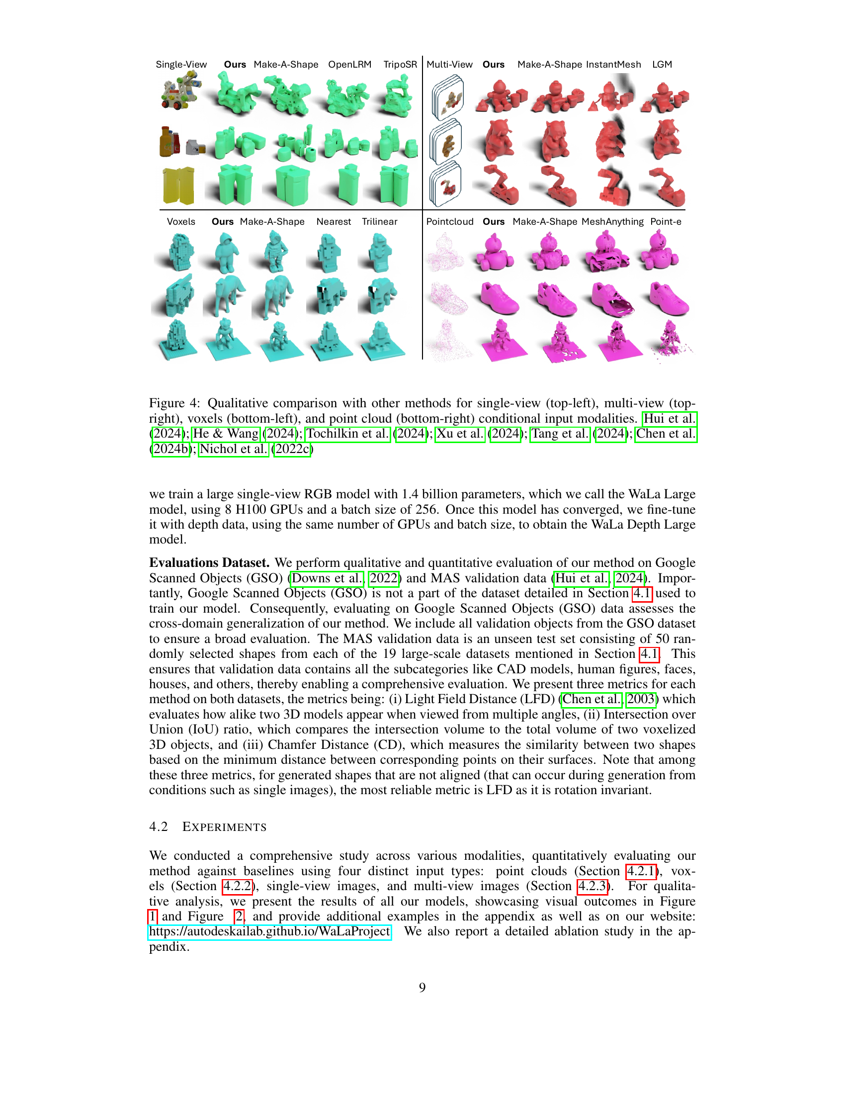
🔼 Figure 4 presents a qualitative comparison of 3D shape generation results using different methods and input modalities. The top-left quadrant shows single-view image input results, comparing the authors’ model (WaLa) against Make-A-Shape, OpenLRM, and TripoSR. The top-right quadrant displays multi-view image input results comparing WaLa to Make-A-Shape and InstantMesh. The bottom-left quadrant showcases voxel input results, comparing WaLa against Make-A-Shape, Nearest, and Trilinear. Finally, the bottom-right quadrant displays point cloud input results comparing WaLa against Make-A-Shape and MeshAnything. This figure visually demonstrates the performance of WaLa compared to other state-of-the-art 3D generative models across various input modalities, highlighting its ability to generate high-quality shapes.
read the caption
Figure 4: Qualitative comparison with other methods for single-view (top-left), multi-view (top-right), voxels (bottom-left), and point cloud (bottom-right) conditional input modalities. Hui et al. (2024); He & Wang (2024); Tochilkin et al. (2024); Xu et al. (2024); Tang et al. (2024); Chen et al. (2024b); Nichol et al. (2022c)

🔼 Figure 5 showcases six distinct methods for generating sketches from a 3D model (mesh from Fu et al., 2021). These methods are: Grease Pencil (a Blender tool creating artistic strokes), Canny edge detection (for outlining shapes), HED (Holistically-Nested Edge Detection, a deep learning technique to highlight edges), HED+potrace (HED output further processed using potrace to clean up the lines), HED+scribble (HED output with a scribble effect), and CLIPasso (a method generating sketches from a depth map, using strokes consistent with a given caption). A reference depth map is also included for comparison.
read the caption
Figure 5: The 6 different sketch types. From left to right: Grease Pencil, Canny, HED, HED+potrace, HED+scribble, CLIPaasso, and a depth map for reference. Mesh taken from (Fu et al., 2021).

🔼 Figure 6 shows the eight different viewpoints from which sketches were generated for use as input to the 3D shape generation model. The images were created using Blender’s Grease Pencil tool, with a mesh from the Fu et al. (2021) paper as the base. The CLIPasso technique, an alternative method for sketch generation, was only used for three of the eight views (the first, fifth, and sixth from the left). These sketches represent a variety of perspectives of the same object used to train the model, which likely helps the model learn to generalize the object from various angles.
read the caption
Figure 6: The 8 different views for which sketches were generated. Images created using the Grease Pencil technique on a mesh taken from Fu et al. (2021). The CLIPasso technique was only used on the first, fifth, and sixth views from the left.

🔼 Figure 7 showcases the model’s ability to generate detailed and diverse 3D shapes from text descriptions. Each row displays a unique text prompt and the corresponding 3D renderings produced by the model. The variety of shapes demonstrates the model’s capacity to handle diverse textual inputs and produce high-quality, detailed outputs.
read the caption
Figure 7: This figure presents more results from the text-to-3D generation task. Each row corresponds to a unique text prompt, with the resulting 3D renderings highlighting the model’s capability to produce detailed and varied shapes from these inputs.

🔼 This figure showcases the model’s ability to generate diverse 3D models from the same text prompt. For each of the listed text prompts, four different 3D variations are shown. Despite the variations, all four models maintain a strong thematic resemblance to the prompt. This demonstrates the model’s flexibility in producing multiple creative and distinct outputs while staying true to the core concept represented in the text.
read the caption
Figure 8: Here, for each caption, four different 3D variations are displayed. This figure emphasizes the model’s flexibility in generating multiple distinct outputs for the same text description while maintaining thematic consistency.

🔼 Figure 9 showcases the model’s ability to generate diverse 3D models from the same text prompt. For each of the nine text prompts shown, four distinct 3D variations are presented. This demonstrates the model’s flexibility and capacity to produce multiple creative outputs while maintaining a consistent theme or concept for each prompt. The variations are subtle yet noticeable, highlighting the model’s ability to explore different interpretations of the same input instruction.
read the caption
Figure 9: Here, for each caption, four different 3D variations are displayed. This figure emphasizes the model’s flexibility in generating multiple distinct outputs for the same text description while maintaining thematic consistency.
More on tables
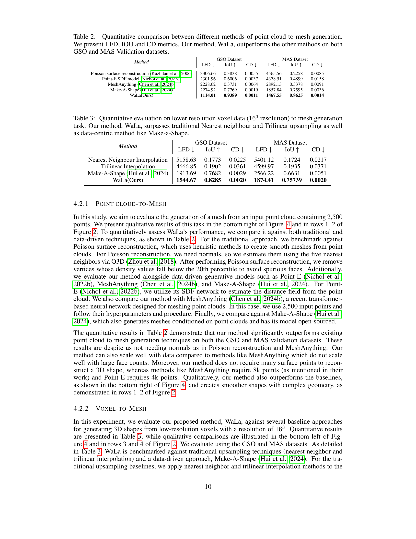
| Method | GSO Dataset LFD ↓ | GSO Dataset IoU ↑ | GSO Dataset CD ↓ | MAS Dataset LFD ↓ | MAS Dataset IoU ↑ | MAS Dataset CD ↓ |
|---|---|---|---|---|---|---|
| Poisson surface reconstruction (Kazhdan et al., 2006) | 3306.66 | 0.3838 | 0.0055 | 4565.56 | 0.2258 | 0.0085 |
| Point-E SDF model (Nichol et al., 2022c) | 2301.96 | 0.6006 | 0.0037 | 4378.51 | 0.4899 | 0.0158 |
| MeshAnything (Chen et al., 2024b) | 2228.62 | 0.3731 | 0.0064 | 2892.13 | 0.3378 | 0.0091 |
| Make-A-Shape (Hui et al., 2024) | 2274.92 | 0.7769 | 0.0019 | 1857.84 | 0.7595 | 0.0036 |
| WaLa(Ours) | 1114.01 | 0.9389 | 0.0011 | 1467.55 | 0.8625 | 0.0014 |
🔼 Table 2 presents a quantitative comparison of various methods used for generating 3D meshes from point cloud data. The comparison uses three key metrics: Light Field Distance (LFD), Intersection over Union (IoU), and Chamfer Distance (CD). Lower LFD and CD values indicate better mesh quality, while higher IoU values suggest more accurate reconstruction of the original shape. The results demonstrate that the Wavelet Latent Diffusion (WaLa) method significantly outperforms other existing techniques on both the Google Scanned Objects (GSO) and MAS validation datasets.
read the caption
Table 2: Quantitative comparison between different methods of point cloud to mesh generation. We present LFD, IOU and CD metrics. Our method, WaLa, outperforms the other methods on both GSO and MAS Validation datasets.
| Method | GSO Dataset LFD ↓ | GSO Dataset IoU ↑ | GSO Dataset CD ↓ | MAS Dataset LFD ↓ | MAS Dataset IoU ↑ | MAS Dataset CD ↓ |
|---|---|---|---|---|---|---|
| Nearest Neighbour Interpolation | 5158.63 | 0.1773 | 0.0225 | 5401.12 | 0.1724 | 0.0217 |
| Trilinear Interpolation | 4666.85 | 0.1902 | 0.0361 | 4599.97 | 0.1935 | 0.0371 |
| Make-A-Shape (Hui et al., 2024) | 1913.69 | 0.7682 | 0.0029 | 2566.22 | 0.6631 | 0.0051 |
| WaLa(Ours) | 1544.67 | 0.8285 | 0.0020 | 1874.41 | 0.75739 | 0.0020 |
🔼 This table presents a quantitative comparison of different methods for generating 3D meshes from low-resolution (16^3) voxel data. The methods compared include traditional upsampling techniques (nearest neighbor and trilinear interpolation) and a data-centric approach (Make-a-Shape). The evaluation metrics used are Light Field Distance (LFD), Intersection over Union (IoU), and Chamfer Distance (CD). The results demonstrate that the Wavelet Latent Diffusion (WaLa) method significantly outperforms the other approaches in terms of mesh quality, as measured by these metrics.
read the caption
Table 3: Quantitative evaluation on lower resolution voxel data (163superscript16316^{3}16 start_POSTSUPERSCRIPT 3 end_POSTSUPERSCRIPT resolution) to mesh generation task. Our method, WaLa, surpasses traditional Nearest neighbour and Trilinear upsampling as well as data-centric method like Make-a-Shape.
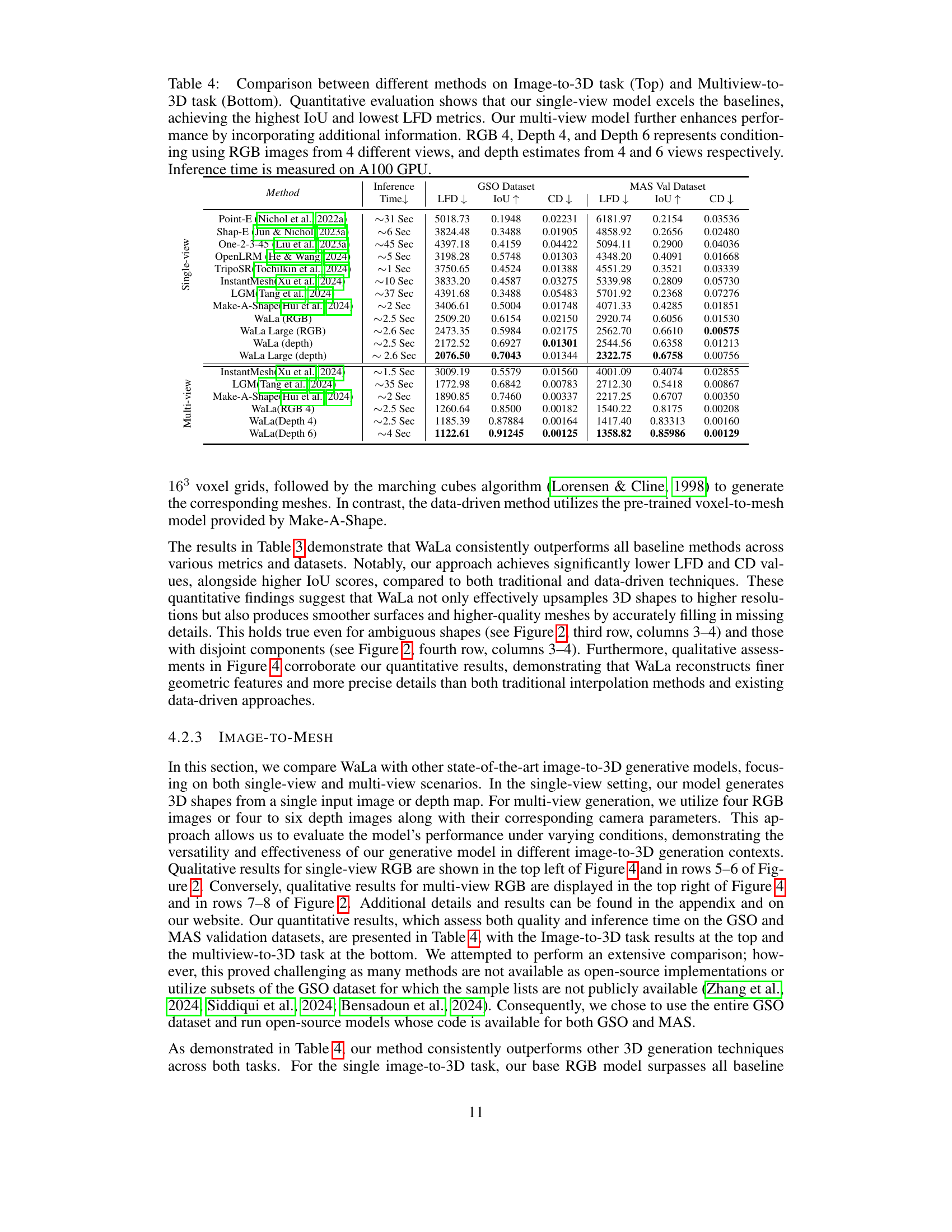
| Method | Inference Time | GSO Dataset LFD↓ | GSO Dataset IoU↑ | GSO Dataset CD↓ | MAS Val Dataset LFD↓ | MAS Val Dataset IoU↑ | MAS Val Dataset CD↓ |
|---|---|---|---|---|---|---|---|
| Point-E (Nichol et al., 2022a) | ~31 Sec | 5018.73 | 0.1948 | 0.02231 | 6181.97 | 0.2154 | 0.03536 |
| Shap-E (Jun & Nichol, 2023a) | ~6 Sec | 3824.48 | 0.3488 | 0.01905 | 4858.92 | 0.2656 | 0.02480 |
| Single-view One-2-3-45 (Liu et al., 2023a) | ~45 Sec | 4397.18 | 0.4159 | 0.04422 | 5094.11 | 0.2900 | 0.04036 |
| OpenLRM (He & Wang, 2024) | ~5 Sec | 3198.28 | 0.5748 | 0.01303 | 4348.20 | 0.4091 | 0.01668 |
| TripoSR (Tochilkin et al., 2024) | ~1 Sec | 3750.65 | 0.4524 | 0.01388 | 4551.29 | 0.3521 | 0.03339 |
| InstantMesh (Xu et al., 2024) | ~10 Sec | 3833.20 | 0.4587 | 0.03275 | 5339.98 | 0.2809 | 0.05730 |
| LGM (Tang et al., 2024) | ~37 Sec | 4391.68 | 0.3488 | 0.05483 | 5701.92 | 0.2368 | 0.07276 |
| Make-A-Shape (Hui et al., 2024) | ~2 Sec | 3406.61 | 0.5004 | 0.01748 | 4071.33 | 0.4285 | 0.01851 |
| WaLa (RGB) | ~2.5 Sec | 2509.20 | 0.6154 | 0.02150 | 2920.74 | 0.6056 | 0.01530 |
| WaLa Large (RGB) | ~2.6 Sec | 2473.35 | 0.5984 | 0.02175 | 2562.70 | 0.6610 | 0.00575 |
| WaLa (depth) | ~2.5 Sec | 2172.52 | 0.6927 | 0.01301 | 2544.56 | 0.6358 | 0.01213 |
| WaLa Large (depth) | ~2.6 Sec | 2076.50 | 0.7043 | 0.01344 | 2322.75 | 0.6758 | 0.00756 |
| InstantMesh (Xu et al., 2024) | ~1.5 Sec | 3009.19 | 0.5579 | 0.01560 | 4001.09 | 0.4074 | 0.02855 |
| Multi-view LGM (Tang et al., 2024) | ~35 Sec | 1772.98 | 0.6842 | 0.00783 | 2712.30 | 0.5418 | 0.00867 |
| Make-A-Shape (Hui et al., 2024) | ~2 Sec | 1890.85 | 0.7460 | 0.00337 | 2217.25 | 0.6707 | 0.00350 |
| WaLa(RGB 4) | ~2.5 Sec | 1260.64 | 0.8500 | 0.00182 | 1540.22 | 0.8175 | 0.00208 |
| WaLa(Depth 4) | ~2.5 Sec | 1185.39 | 0.87884 | 0.00164 | 1417.40 | 0.83313 | 0.00160 |
| WaLa(Depth 6) | ~4 Sec | 1122.61 | 0.91245 | 0.00125 | 1358.82 | 0.85986 | 0.00129 |
🔼 Table 4 presents a quantitative comparison of various methods for generating 3D models from images, specifically focusing on single-view and multi-view scenarios. The key performance indicators are the Intersection over Union (IoU), measuring the overlap between the generated and ground truth 3D models, and the Light Field Distance (LFD), representing the dissimilarity in appearance from multiple viewpoints. The table demonstrates that the proposed Wavelet Latent Diffusion (WaLa) model significantly outperforms existing methods in both single-view and multi-view settings. The improvement in multi-view is attributed to the inclusion of additional information from multiple perspectives. Different conditioning strategies are explored using RGB images and depth estimations from varying numbers of views. Inference times are also provided, all measured using an A100 GPU.
read the caption
Table 4: Comparison between different methods on Image-to-3D task (Top) and Multiview-to-3D task (Bottom). Quantitative evaluation shows that our single-view model excels the baselines, achieving the highest IoU and lowest LFD metrics. Our multi-view model further enhances performance by incorporating additional information. RGB 4, Depth 4, and Depth 6 represents conditioning using RGB images from 4 different views, and depth estimates from 4 and 6 views respectively. Inference time is measured on A100 GPU.
| Sampling Loss | Amount of finetune data | IOU ↑ | MSE ↓ | D-IOU ↑ | D-MSE ↓ |
|---|---|---|---|---|---|
| No1 | - | 0.91597 | 0.00270 | 0.91597 | 0.00270 |
| Yes1 | - | 0.92619 | 0.00136 | 0.91754 | 0.00229 |
| Yes | - | 0.95479 | 0.00090 | 0.94093 | 0.00169 |
| Yes | 2500 | 0.95966 | 0.00078 | 0.94808 | 0.00149 |
| Yes | 5000 | 0.95873 | 0.00078 | 0.94793 | 0.00149 |
| Yes | 10000 | 0.95979 | 0.00078 | 0.94820 | 0.00148 |
| Yes | 20000 | 0.95707 | 0.00079 | 0.94659 | 0.00150 |
1Results for the first two rows are based on 200k iterations.
🔼 This table presents the results of an ablation study conducted to evaluate the impact of adaptive sampling loss and VQ-VAE finetuning on the performance of the model. It shows how different combinations of these techniques affect the model’s ability to reconstruct shapes accurately, as measured by Intersection over Union (IoU) and Mean Squared Error (MSE). The study also considers D-IoU and D-MSE metrics, which take data imbalance into account. The results demonstrate the effectiveness of adaptive sampling loss and balanced fine-tuning for improved accuracy.
read the caption
Table 5: Ablation study on adaptive sampling as well finetuning of the VQ-VAE model.
| Architecture | hidden dim | No. of layers | post or pre | LFD ↓ | IoU ↑ | CD ↓ |
|---|---|---|---|---|---|---|
| U-VIT | 384 | 32 | pre | 1523.74 | 0.8211 | 0.001544 |
| U-VIT | 768 | 32 | pre | 1618.73 | 0.7966 | 0.001540 |
| U-VIT | 1152 | 8 | pre | 1596.88 | 0.8020 | 0.001561 |
| U-VIT | 1152 | 16 | pre | 1521.81 | 0.8237 | 0.001573 |
| U-VIT | 1152 | 32 | pre | 1507.43 | 0.8199 | 0.001482 |
| DiT | 1152 | 32 | pre | 1527.16 | 0.8145 | 0.001602 |
| U-VIT | 1152 | 32 | post | 1576.07 | 0.8176 | 0.001695 |
🔼 This ablation study investigates the impact of different design choices on the generative model’s performance. It examines the effects of varying the hidden dimension and the number of layers in the U-ViT architecture, comparing the results with a DiT architecture. It also explores the impact of applying the generative model before or after quantization and the effect of using a different number of layers in the attention block.
read the caption
Table 6: Ablation study on the generative model design choices.
| Method | Number of Parameters |
|---|---|
| Autoencoder Model | 12.9 million |
| Uncondition Model | 1.1 billion |
| Single View Model | 956 million |
| Single View Model Large | 1.4 billion |
| Depth View Model | 956 million |
| Depth View Model Large | 1.4 billion |
| Pointcloud Model | 966.7 million |
| Multi View Model (Depth and Image) | 956 million |
| 6 view Depth Model | 898 million |
| Voxel Model | 906.9 million |
🔼 This table presents the number of parameters used in each of the models developed in the study. It breaks down the model sizes for different model types including the autoencoder, various conditional models (single-view image, depth, multi-view), an unconditional model and the voxel model, providing a clear view of the model complexity and scale for each task.
read the caption
Table 7: Number of Parameters for Different Models
| Model | Scale | Timestep |
|---|---|---|
| Voxel | 1.5 | 5 |
| Pointcloud | 1.3 | 8 |
| Single-View RGB | 1.8 | 5 |
| Single-View Depth | 1.8 | 5 |
| Multi-View RGB | 1.3 | 5 |
| Multi-View Depth | 1.3 | 5 |
| 6 Multi-View Depth | 1.5 | 10 |
| Unconditional | - | 1000 |
🔼 This table lists the hyperparameters used for the classifier-free guidance in the diffusion model during inference. Specifically, it shows the classifier-free guidance scale and the number of timesteps used for generating 3D shapes from different input modalities, including voxels, point clouds, single-view and multi-view RGB images, and multi-view depth maps, as well as for unconditional generation.
read the caption
Table 8: Classifier free scale and timestep used in the paper
Full paper#
