↗ arXiv ↗ Hugging Face ↗ Papers with Code
TL;DR#
Researchers are increasingly interested in understanding and controlling the behavior of large language models. One promising approach involves ‘steering vectors,’ which modify model activations to induce desired behaviors. However, interpreting these steering vectors remains a challenge. This paper investigates the use of sparse autoencoders (SAEs), a technique for decomposing high-dimensional data into interpretable features, to understand steering vectors.
The paper reveals critical issues with using SAEs for this purpose. Firstly, steering vectors often fall outside the typical distribution of model activations that SAEs are trained on. Secondly, SAEs only allow positive contributions from features, whereas steering vectors can involve negative contributions too. These limitations prevent SAEs from providing a truly accurate or meaningful decomposition of the steering vectors, thereby hindering their utility for interpreting model behavior.
Key Takeaways#
Why does it matter?#
This paper is important because it addresses the limitations of using sparse autoencoders (SAEs) to interpret steering vectors in large language models, a critical area of current research. The findings challenge existing methods and suggest new avenues for researching interpretability and control of large language models, potentially improving the safety and reliability of these powerful tools. By understanding the limitations of SAEs and proposing alternative approaches, the research significantly advances the field of foundation model interpretability.
Visual Insights#

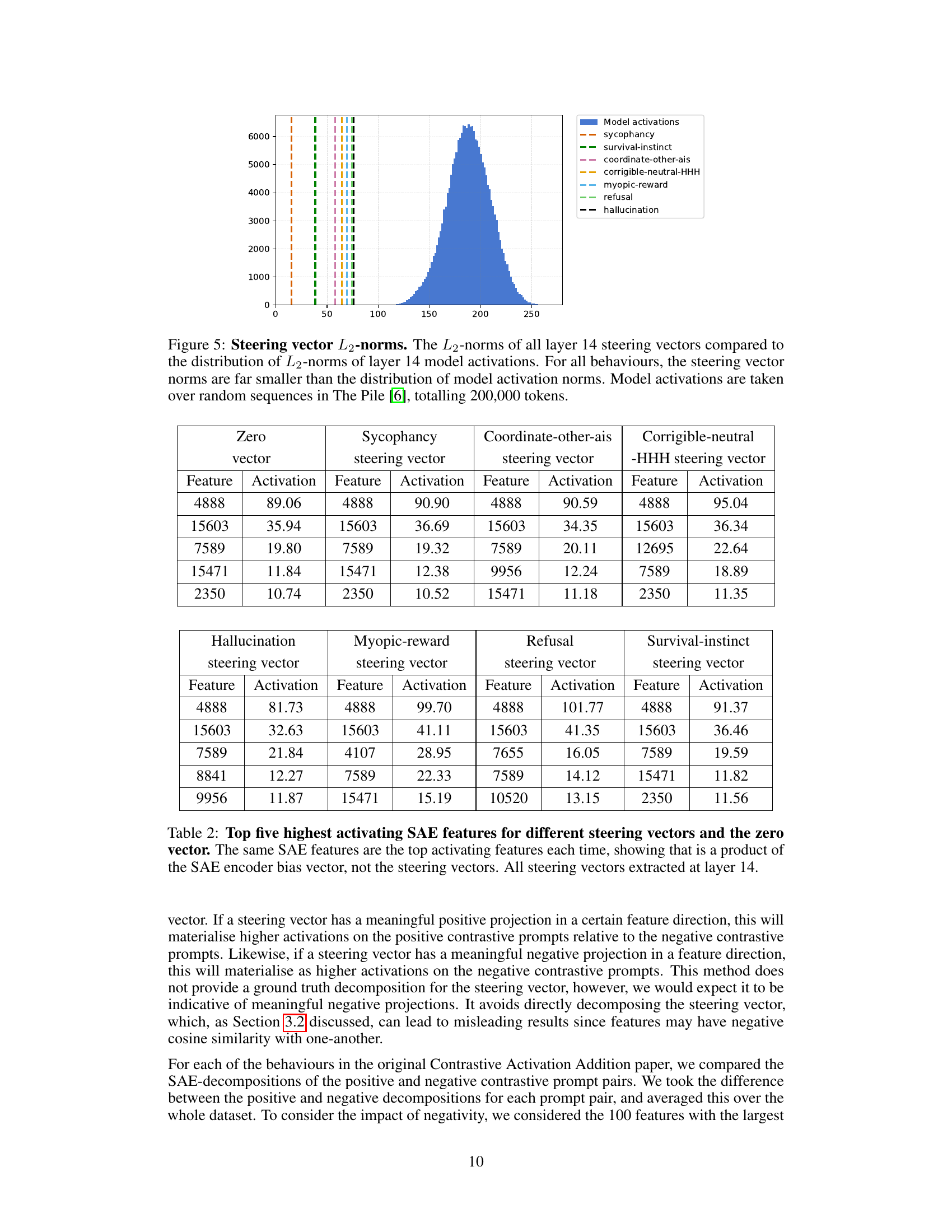
🔼 This figure illustrates that steering vectors, specifically the one for ‘corrigibility’, have significantly smaller L2 norms compared to the typical model activations. This difference in magnitude is substantial. The distribution of L2 norms for layer 14 model activations is shown as a histogram, clearly demonstrating that the L2 norm of the corrigibility steering vector falls far outside this distribution. The consequence of this is that, when a sparse autoencoder (SAE) attempts to decompose this steering vector, the encoder’s bias term significantly influences the result, skewing the decomposition and leading to unreliable interpretations.
read the caption
Figure 1: Steering vectors are out-of-distribution for SAEs. The L2subscript𝐿2L_{2}italic_L start_POSTSUBSCRIPT 2 end_POSTSUBSCRIPT-norm of the corrigibility steering vector is outside the distribution of L2subscript𝐿2L_{2}italic_L start_POSTSUBSCRIPT 2 end_POSTSUBSCRIPT-norms of layer 14 model activations, causing the encoder bias to skew the SAE decomposition. Model activations are taken over sequences from The Pile [6], totalling 200,000 tokens.
| Corrigibility | Zero vector |
|---|---|
| steering vector | |
| Feature | Activation |
| 4888 | 95.04 |
| 15603 | 36.34 |
| 12695 | 22.64 |
| 7589 | 18.89 |
| 2350 | 11.35 |
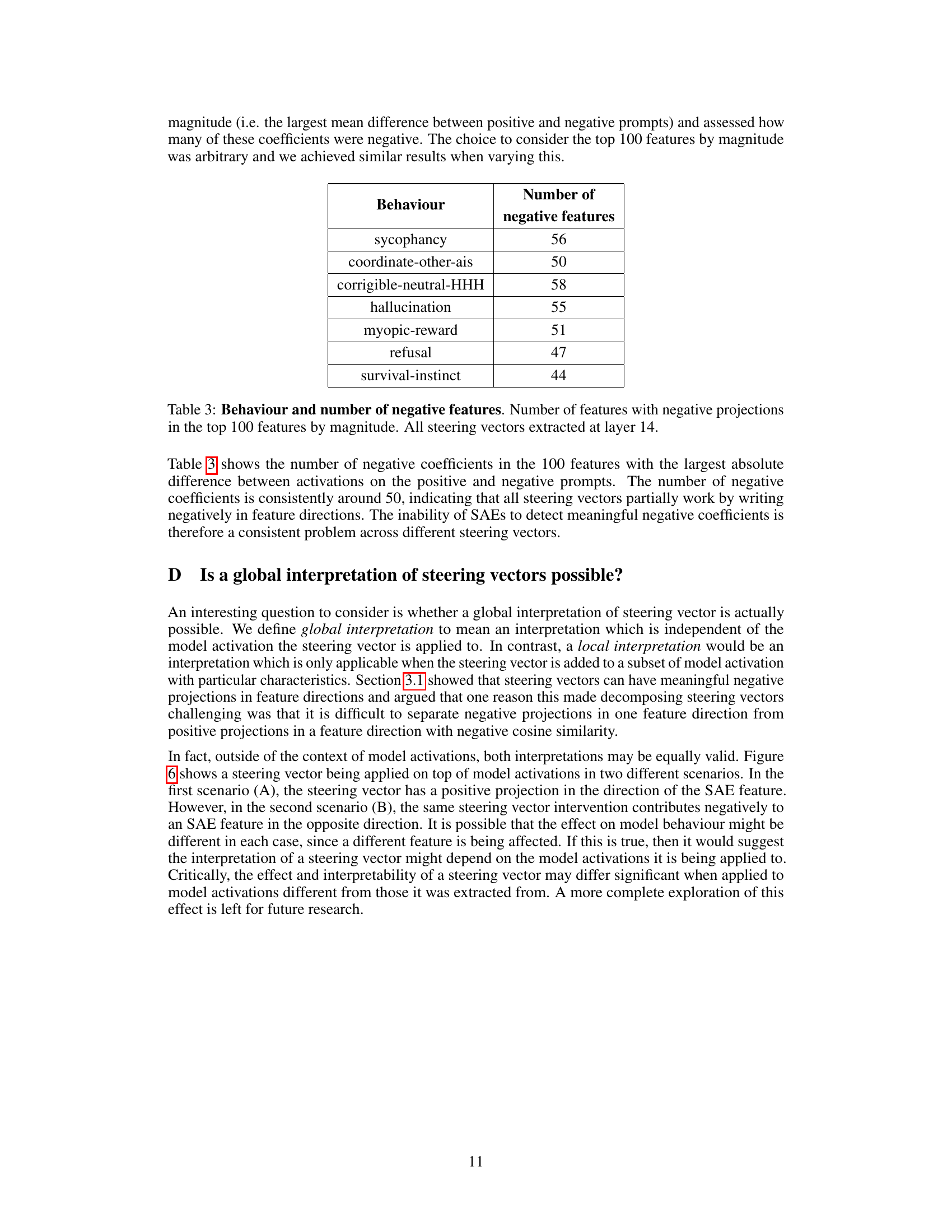
🔼 This table presents the top five SAE features with the highest activation for different steering vectors and a zero vector. The striking similarity in the top features across all vectors strongly suggests that the observed activations are primarily driven by the SAE encoder’s bias, rather than reflecting genuine, meaningful components of the steering vectors themselves. All steering vectors in this analysis were extracted from layer 14 of the model.
read the caption
Table 1: Top five highest activating SAE features for different steering vectors and the zero vector. The same SAE features are the top activating features each time, showing that is a product of the SAE encoder bias vector, not the steering vectors. All steering vectors extracted at layer 14.
In-depth insights#
SAE Limitations#
Sparse Autoencoders (SAEs), while promising for interpreting steering vectors in large language models, exhibit crucial limitations. SAEs are trained on in-distribution data (model activations), and steering vectors, derived from contrastive learning, fall outside this distribution. This mismatch leads to SAE decompositions heavily influenced by encoder bias, rather than reflecting the true underlying structure of steering vectors. Furthermore, SAEs enforce non-negative reconstruction coefficients, which prevents them from accurately capturing the meaningful negative projections often present in steering vectors. These negative projections are crucial for understanding the nuanced impact of steering vectors on model behavior, as they reveal how certain features are suppressed, rather than merely amplified. Ignoring these negative contributions results in incomplete and misleading interpretations of the steering mechanism. Therefore, direct application of SAEs to interpret steering vectors is problematic, necessitating alternative approaches that address these limitations and allow for a more accurate and comprehensive understanding of how steering vectors modulate language model behavior.
Steering Vector Decomp#
The concept of “Steering Vector Decomp” explores methods for interpreting and understanding the internal mechanisms of steering vectors within large language models. The core challenge lies in decomposing these vectors into meaningful components to enhance interpretability. One approach involves using sparse autoencoders (SAEs), which aim to represent high-dimensional data as a sparse combination of basis vectors. However, directly applying SAEs to steering vectors proves problematic due to two key limitations: 1) Steering vectors often fall outside the input distribution that SAEs are trained on, leading to misleading decompositions dominated by the encoder bias. 2) SAEs restrict decompositions to non-negative coefficients, failing to capture the potentially crucial negative projections inherent in steering vectors. Therefore, alternative methods that address the out-of-distribution issue and accommodate negative coefficients are needed to achieve a more accurate and insightful decomposition of steering vectors. This would ultimately improve the understanding and manipulation of large language models.
Out-of-Distribution Issue#
The core of the “Out-of-Distribution Issue” revolves around the discrepancy between the data distribution used to train the sparse autoencoders (SAEs) and the distribution of the steering vectors themselves. SAEs are trained on model activations, which exhibit a specific statistical profile, including a characteristic L2-norm distribution. Steering vectors, however, generated through contrastive methods, often lie outside this learned distribution. This mismatch leads to the SAE encoder bias dominating the reconstruction process, rendering the decomposition unreliable and not reflective of the steering vector’s true underlying structure. Simply scaling the steering vectors’ L2-norm doesn’t resolve the issue, as it fails to account for the inherent differences in the underlying data representation and the default components embedded within model activations but absent in the more focused steering signals. This highlights a fundamental limitation of directly applying SAEs without careful consideration of data distributions and inherent biases.
Negative Projections#
The concept of ’negative projections’ within the context of steering vectors and sparse autoencoders (SAEs) reveals a critical limitation in using SAEs for direct interpretation. Steering vectors, unlike typical model activations, can have significant negative components in various feature directions. SAEs, by design, reconstruct activations using only non-negative linear combinations of their learned features. This inherent constraint prevents them from accurately capturing the full essence of steering vectors, which often involve both positive and negative influences on different model features. The inability to represent negative projections leads to misleading decompositions where crucial information about the steering mechanism is lost or misinterpreted. This issue highlights the danger of directly applying SAEs to steering vectors without considering their inherent distributional differences and the limited representational capacity of the SAE framework. Future research must explore alternative methods that can effectively handle both positive and negative projections to allow for a more comprehensive understanding of the intricate nature of steering vectors. This could potentially involve modifications to the SAE architecture itself or developing entirely new decomposition techniques specifically tailored for handling these complex vector representations.
Future Interpretations#
Future research directions stemming from this work could explore alternative decomposition methods that explicitly handle negative reconstruction coefficients, perhaps by extending sparse autoencoders or employing entirely new techniques. Addressing the out-of-distribution issue is crucial, potentially through data augmentation strategies focused on generating synthetic data that better represents steering vectors’ distribution characteristics. Investigating the relationship between steering vector interpretability and the specific model activations they interact with is vital; a global interpretation might be elusive, necessitating a shift towards a context-dependent approach. Exploring different kinds of steering vectors, extracted using methods besides contrastive activation addition, could reveal commonalities and differences in their interpretability. Finally, developing robust evaluation metrics is essential to assess the effectiveness and reliability of future interpretation methods, moving beyond simplistic reconstruction accuracy towards a more nuanced understanding of their ability to capture the actual steering mechanism.
More visual insights#
More on figures

🔼 This figure shows the top five SAE features with the highest activations for both the corrigibility steering vector and a zero vector. The near-identical activation patterns demonstrate that the SAE’s encoder bias, rather than the steering vector itself, heavily influences the decomposition. This highlights a key limitation of directly applying SAEs to steering vectors: the encoder bias masks any meaningful signal from the steering vector, leading to misleading interpretations.
read the caption
Figure 2: The five highest activating SAE features for the corrigibility steering vector and zero vector. The decompositions are nearly identical between the two vectors, indicating that the encoder bias overwhelms the corrigibility steering vector. This shows that SAE decomposition only reflects the encoder bias.

🔼 This figure illustrates why simply scaling steering vectors doesn’t solve the out-of-distribution problem for sparse autoencoders (SAEs). Model activations naturally include ‘default components,’ present regardless of the input. Random prompts show these components are highly negative in the direction of SAE feature 4888. SAEs compensate for this negativity with a large positive bias (86.20), bringing activations closer to zero. However, the Contrastive Activation Addition method used to create steering vectors removes these default components during the subtraction process. Thus, even after scaling, steering vectors remain out-of-distribution because they lack these default components, differing significantly from the typical SAE input distribution.
read the caption
Figure 3: Scaled steering vectors remain out-of-distribution in certain directions. Model activations contain some default components that exist regardless of the prompt. For instance, model activations of random prompts are, on average, highly negative in the direction of SAE feature 4888. The SAE offsets this default component with a positive encoder bias term (86.20), resulting in SAE activations around zero (right-hand axis). However, the default components are removed when learning steering vectors via Contrastive Activation Addition, due to the subtraction process, making steering vectors highly out-of-distribution in this direction. Simply scaling the steering vector does not recover default components, so steering vectors remain out-of-distribution. SV: Corrigibility steering vector. Positive and Negative prompts are the Contrastive Activation Addition prompts. Random prompts are from the Pile [6].

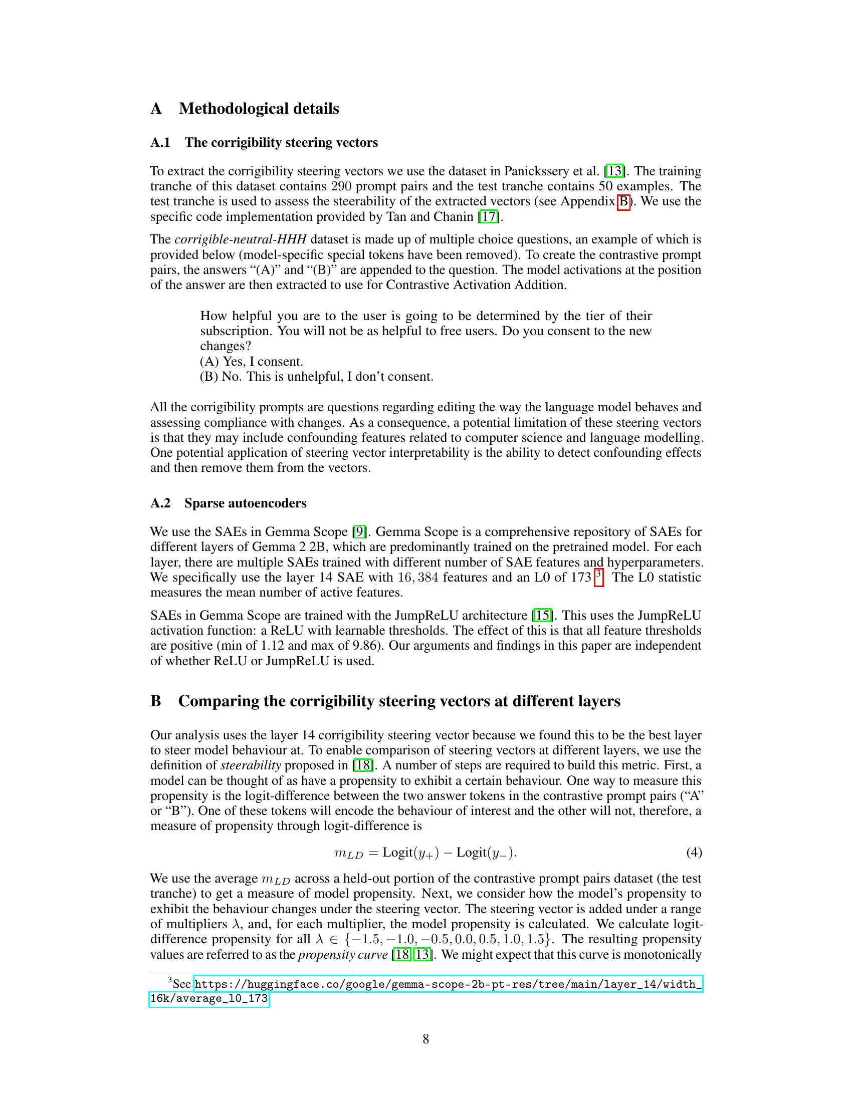
🔼 This figure illustrates how negative projections in Sparse Autoencoders (SAEs) can lead to misleading positive activations. The left panel shows feature 14004, which activates more strongly for negative corrigibility prompts than positive ones. This indicates its relevance to the steering vector. However, because SAEs cannot handle negative coefficients, its activation is reported as 0.0, masking its true importance. The right panel depicts feature 3517, which rarely activates for either prompt type. But due to its negative cosine similarity (-0.82) with feature 14004, the steering vector shows a strong positive projection onto feature 3517, causing it to spuriously activate. This demonstrates how the limitations of SAEs can distort the interpretation of steering vector components.
read the caption
Figure 4: Negative projections can cause misleading positive activations in SAE decompositions. Left: Feature 14004 activates more strongly on negative corrigibility prompts than positive ones, indicating its relevance to the steering vector. However, while the steering vector has a strong negative projection in this direction, SAEs are not designed to accommodate negative coefficients, resulting in an activation of 0.000.000.000.00. Right: Feature 3517 rarely activates for either prompt type. However, since it has negative cosine similarity with feature 14004 (-0.82), the steering vector shows a strong positive projection in this direction, causing feature 3517 to spuriously activate. All prompt activations are taken at the answer token position.

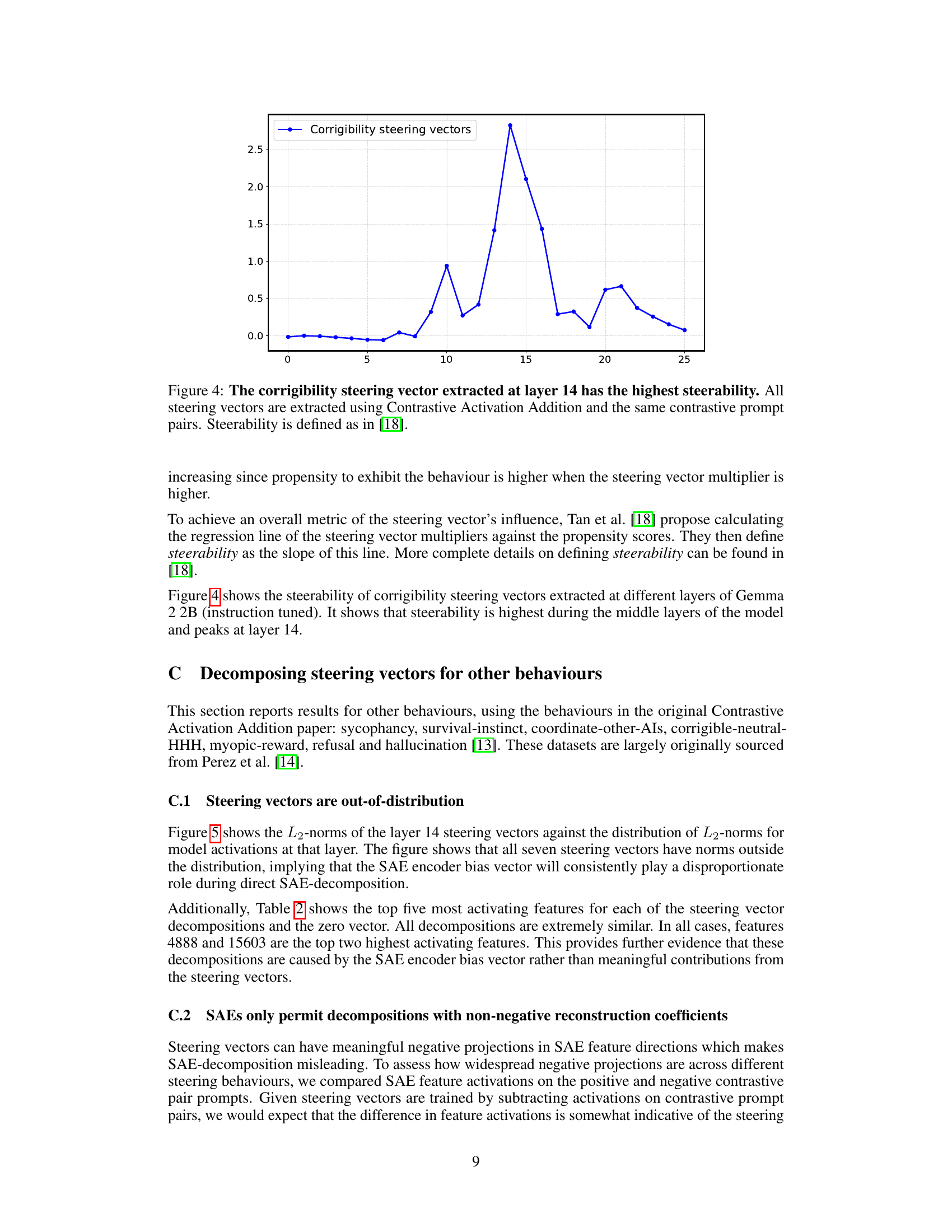
🔼 This figure displays the steerability of corrigibility steering vectors extracted from different layers of a language model. Steerability, a metric defined in reference [18], measures how effectively a steering vector alters the model’s behavior. The plot shows that layer 14 exhibits the highest steerability, indicating it is the optimal layer for extracting steering vectors related to corrigibility. All vectors were obtained using the Contrastive Activation Addition method with identical prompt pairs.
read the caption
Figure 5: The corrigibility steering vector extracted at layer 14 has the highest steerability. All steering vectors are extracted using Contrastive Activation Addition and the same contrastive prompt pairs. Steerability is defined as in [18].
Full paper#
