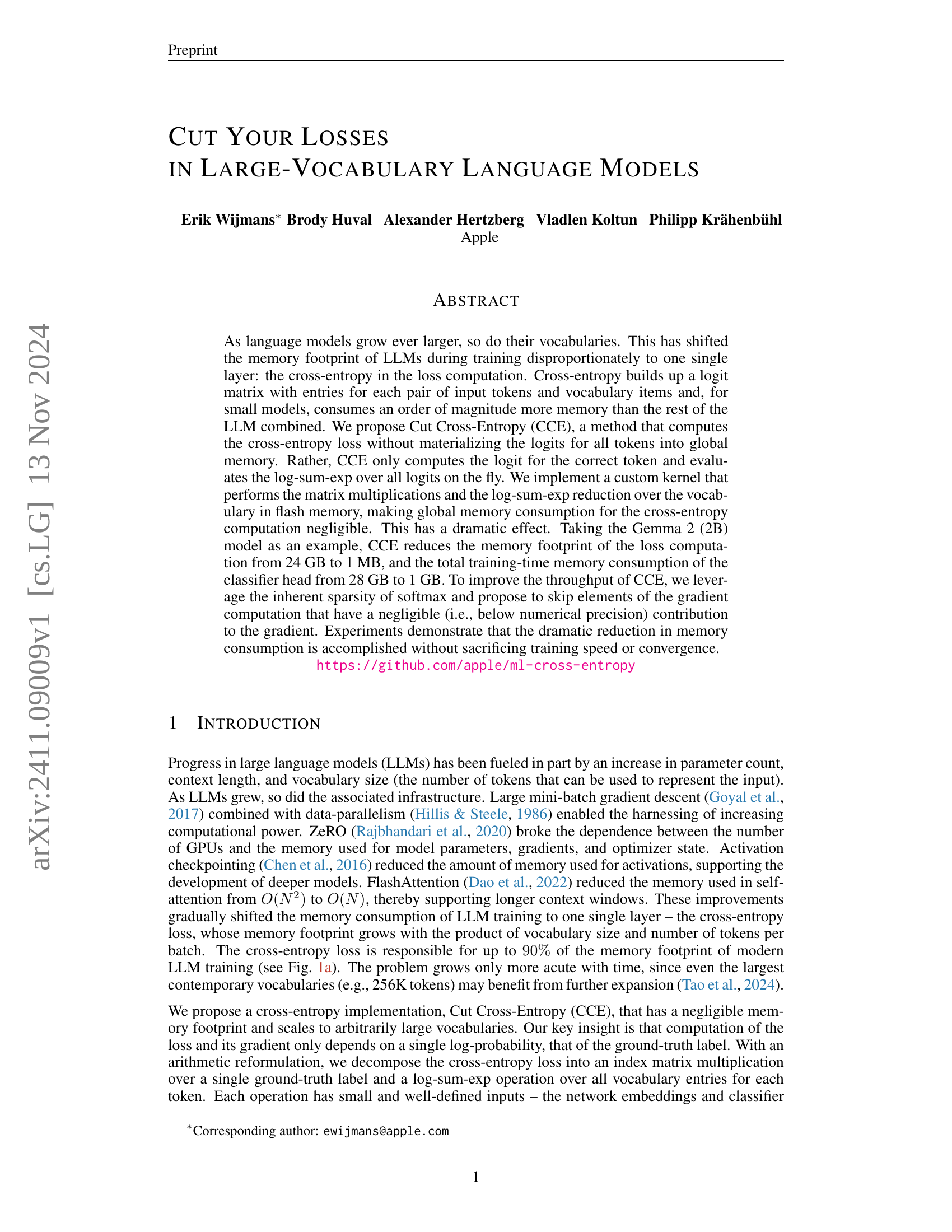
↗ arXiv ↗ Hugging Face ↗ Papers with Code
TL;DR#
Training large language models (LLMs) is computationally expensive, particularly as vocabulary sizes grow. A major memory bottleneck arises from the cross-entropy loss calculation, which requires storing a large logit matrix. This limits the scalability of LLMs and restricts the use of bigger batch sizes. Existing techniques to address this involve trade-offs between memory and latency.
The paper introduces Cut Cross-Entropy (CCE), a novel method to tackle this memory limitation. CCE cleverly reformulates the cross-entropy calculation to avoid creating the large logit matrix, instead computing logits on-the-fly. It employs custom kernels to perform matrix multiplications and log-sum-exp reductions in fast memory, significantly reducing the memory footprint. Experiments show that CCE drastically reduces memory usage without compromising training speed or convergence, paving the way for training larger, more powerful LLMs.
Key Takeaways#
Why does it matter?#
This paper is crucial for researchers working with large language models (LLMs) because it directly addresses the significant memory bottleneck in training LLMs with large vocabularies. The proposed Cut Cross-Entropy (CCE) method offers a practical solution to a major scalability challenge, enabling the training of even larger and more powerful LLMs. Furthermore, the techniques used in CCE, such as gradient filtering and vocabulary sorting, are applicable to other memory-intensive machine learning tasks. This makes it highly relevant to current research trends in efficient deep learning.
Visual Insights#

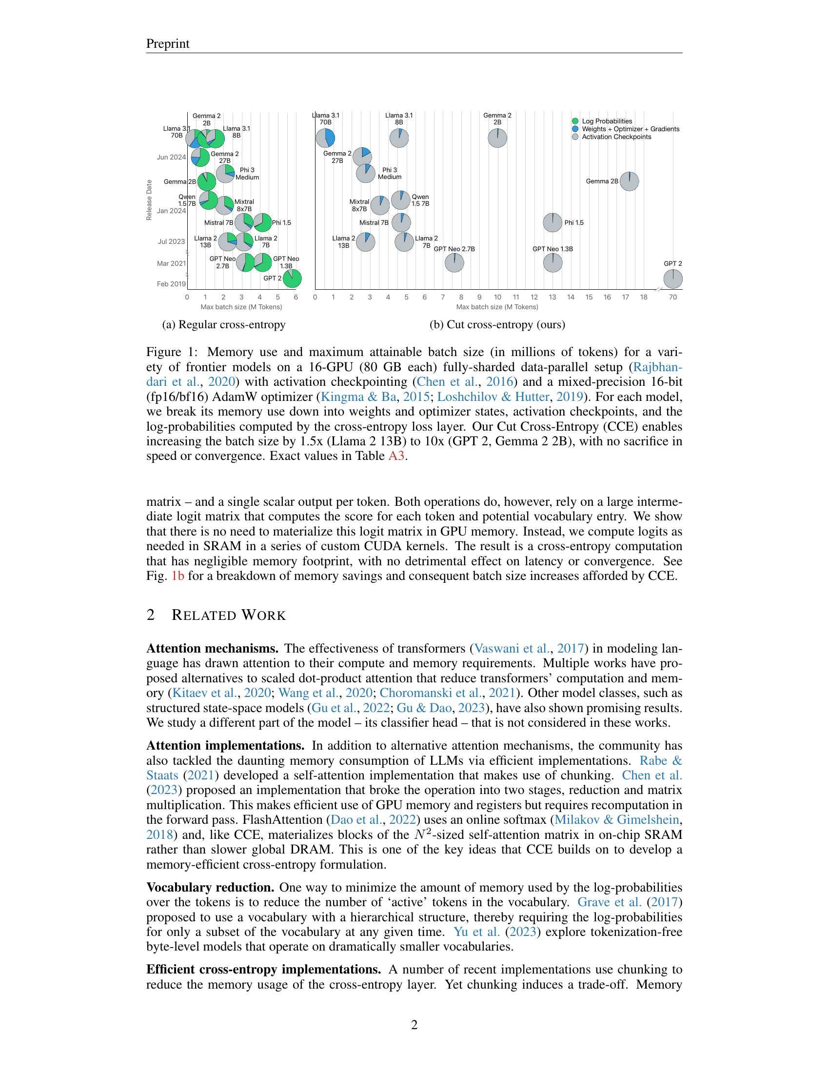
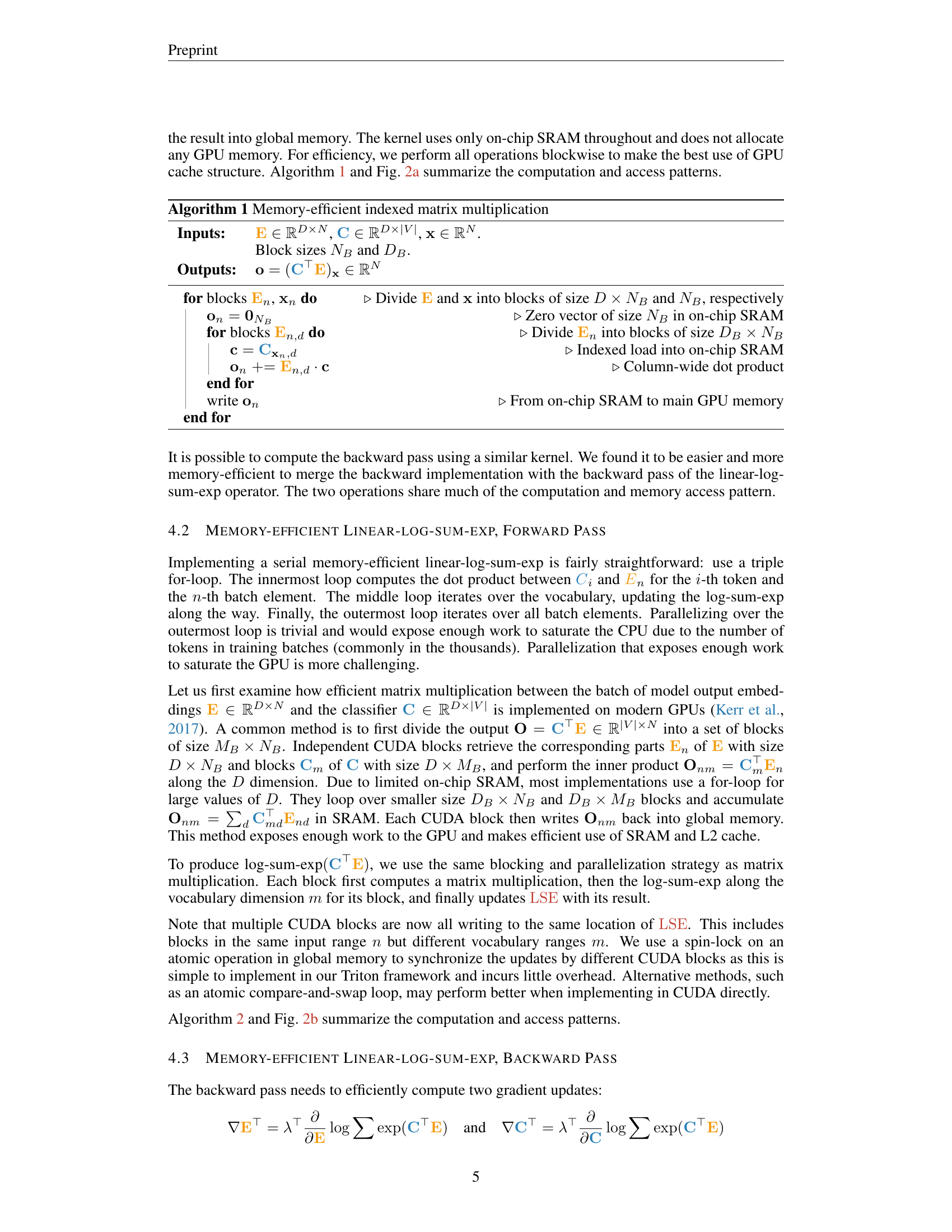
🔼 This figure shows a comparison of memory usage for different language models using regular cross-entropy and the proposed Cut Cross-Entropy (CCE). Subfigure (a) displays memory usage for various models when using the standard cross-entropy loss computation. It breaks down the memory usage into different components: log probabilities, weights and optimizer states, and activation checkpoints. The x-axis represents the maximum batch size in millions of tokens, while the y-axis represents the memory usage in gigabytes (GB). Each point represents a specific language model. The different colored parts of the points represent the memory consumption of each part of the model. The subfigure shows that the log probabilities of the cross-entropy loss consume a significant portion of the memory.
read the caption
(a) Regular cross-entropy
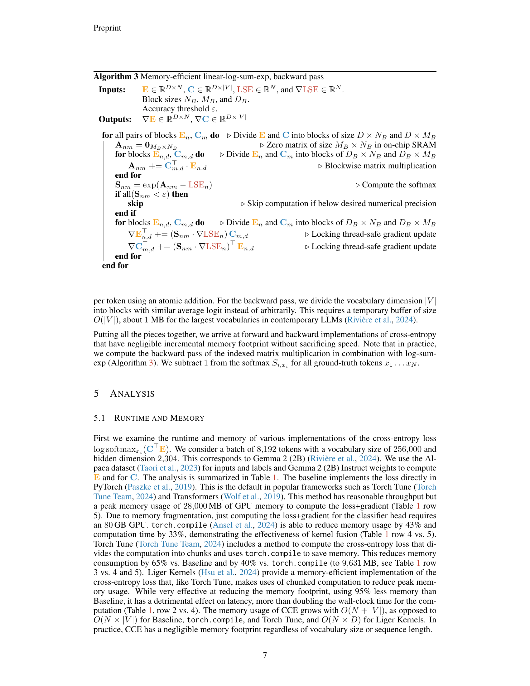
🔼 This table compares the peak memory usage and runtime for different methods of computing the cross-entropy loss and its gradient. It includes a baseline PyTorch implementation, optimized versions using
torch.compileand Torch Tune, the Liger Kernels approach, and the proposed Cut Cross-Entropy (CCE) method. The comparison considers memory usage for the loss computation, gradient calculation, and their combination. The experiment used a batch size of 8192 tokens and a vocabulary size of 256,000, with a hidden dimension of 2304, running on an A100-SXM4 GPU with 80GB of RAM. The lower bound represents the minimum memory needed for the output gradients. Note that memory reuse between loss and gradient computations can sometimes reduce the overall peak memory.read the caption
Table 1: Peak memory footprint and time to compute the loss, its gradient, and their combination. Note that intermediate buffers can often (but not always) be reused between the loss and gradient computation, resulting in lower peak memory consumption than the sum of the parts. Batch of 8192819281928192 tokens with a vocabulary size of 256000256000256000256000 and hidden dimension 2304. Embedding and classifier matrix taken during Gemma 2 (2B) training on Alpaca. Measured on an A100-SXM4 GPU with \qty80GB of RAM, PyTorch 2.4.1, CUDA 12.4, rounded to closest MB. Some numbers are multiples of 1000100010001000 due to dimensions chosen and PyTorch’s allocation strategy. ‘Lower bound’ is the amount of memory required for the output buffer(s), i.e., ∇𝐄∇𝐄\nabla\mathbf{{\color[rgb]{0.953125,0.61328125,0.0703125}\definecolor[named]{% pgfstrokecolor}{rgb}{0.953125,0.61328125,0.0703125}E}}∇ bold_E and ∇𝐂∇𝐂\nabla\mathbf{{\color[rgb]{0.16015625,0.5,0.7265625}\definecolor[named]{% pgfstrokecolor}{rgb}{0.16015625,0.5,0.7265625}C}}∇ bold_C, this is the lower bound for the memory footprint of any method.
In-depth insights#
Cross-Entropy Bottleneck#
The concept of a “Cross-Entropy Bottleneck” in large language models (LLMs) highlights a critical performance limitation. The cross-entropy loss calculation, a core component of LLM training, becomes increasingly memory-intensive as vocabulary size grows. This is because it requires constructing and storing a large logit matrix, representing the probabilities of all vocabulary items for each input token. This memory constraint directly impacts the ability to train models with massive vocabularies and large batch sizes. The bottleneck stems from the quadratic relationship between memory consumption and both vocabulary size and batch size. Addressing this bottleneck is crucial for advancing the field, as it significantly limits the scalability of LLM training. Solutions explored often involve clever memory management techniques, exploiting sparsity inherent in softmax calculations, or alternative loss functions entirely. Ultimately, overcoming this bottleneck is key to unlocking the potential of even larger and more powerful LLMs.
CCE: Memory-Efficient#
The heading ‘CCE: Memory-Efficient’ suggests a focus on a novel technique, Cut Cross-Entropy (CCE), designed to drastically reduce memory consumption in large language models (LLMs). The core innovation likely involves optimizing the computation of cross-entropy loss, a major memory bottleneck in LLMs, especially those with extensive vocabularies. Instead of materializing the entire logit matrix in global memory, which is computationally expensive, CCE probably employs a more efficient strategy. This might involve clever reformulations of the cross-entropy calculation, possibly leveraging efficient computation on-chip SRAM. The method’s memory efficiency is expected to significantly boost training throughput and enable scaling to even larger vocabularies. The reduction in memory footprint would likely translate to an increase in the maximum batch size attainable during training, a critical factor impacting model convergence speed. Furthermore, CCE’s memory efficiency likely comes without sacrificing training speed or accuracy, which is a significant accomplishment. Additional optimizations might be incorporated to further improve efficiency, such as techniques exploiting the sparsity of softmax and gradient filtering.
Sparsity Exploitation#
Sparsity exploitation is a crucial technique for optimizing large language models (LLMs). The inherent sparsity in the softmax probabilities, particularly in the context of a large vocabulary, can be leveraged to significantly reduce computational costs and memory consumption. By identifying and ignoring elements of the gradient with negligible contributions, gradient filtering effectively speeds up the backpropagation process. Furthermore, smart vocabulary sorting can group frequently used tokens together, enhancing the efficiency of blockwise operations and reducing data access latency. These optimization methods are vital for training and deploying LLMs with expansive vocabularies, making it feasible to achieve substantial gains in efficiency and memory management without significant loss in accuracy. The interplay between gradient filtering and vocabulary sorting allows the system to maximize the benefits of sparsity, highlighting the importance of a holistic approach in LLM optimization.
Gradient Filtering#
Gradient filtering, as described in the context of this research paper, is a crucial optimization technique designed to enhance the efficiency of the backpropagation process in large language models (LLMs). It leverages the inherent sparsity of the softmax probability distribution, recognizing that many gradient components are below numerical precision and thus inconsequential to the overall gradient update. By skipping these negligible elements, gradient filtering dramatically reduces the computational cost and memory footprint associated with the backpropagation step. This is particularly beneficial for LLMs with vast vocabularies, where the softmax calculation can become a computational bottleneck. The effectiveness of this technique stems from the observation that the softmax probabilities decay rapidly, making many elements effectively zero. The research demonstrates that this filtering process leads to significant speed improvements without compromising training convergence or accuracy. The thoughtful design of this method highlights the importance of exploiting inherent properties of the data to optimize resource consumption and training time. The combination of this technique with other optimizations, such as vocabulary sorting, further demonstrates a commitment to comprehensive system optimization for training efficiency.
Future: Extensibility#
The heading ‘Future: Extensibility’ suggests a discussion on the scalability and adaptability of the research’s contributions. A thoughtful analysis would explore how the presented methods or models can handle future growth in data size, model complexity, or vocabulary size. Key aspects to consider would be the computational cost and memory requirements as these factors scale. The analysis should investigate whether the proposed techniques remain efficient and practical under these conditions. A critical point would be an assessment of the algorithm’s ability to accommodate new features or functionalities without requiring substantial redesign. Does the architecture allow for seamless integration of improved components or advancements in related fields? Furthermore, the discussion should consider the ease of implementation and deployment. Is the technology sufficiently modular and flexible to be adopted by diverse users and integrated with existing systems? Finally, exploring limitations is crucial. Are there inherent constraints that may prevent widespread adoption or limit scalability in specific scenarios? Addressing these aspects would provide a robust evaluation of the research’s long-term viability and potential impact.
More visual insights#
More on figures
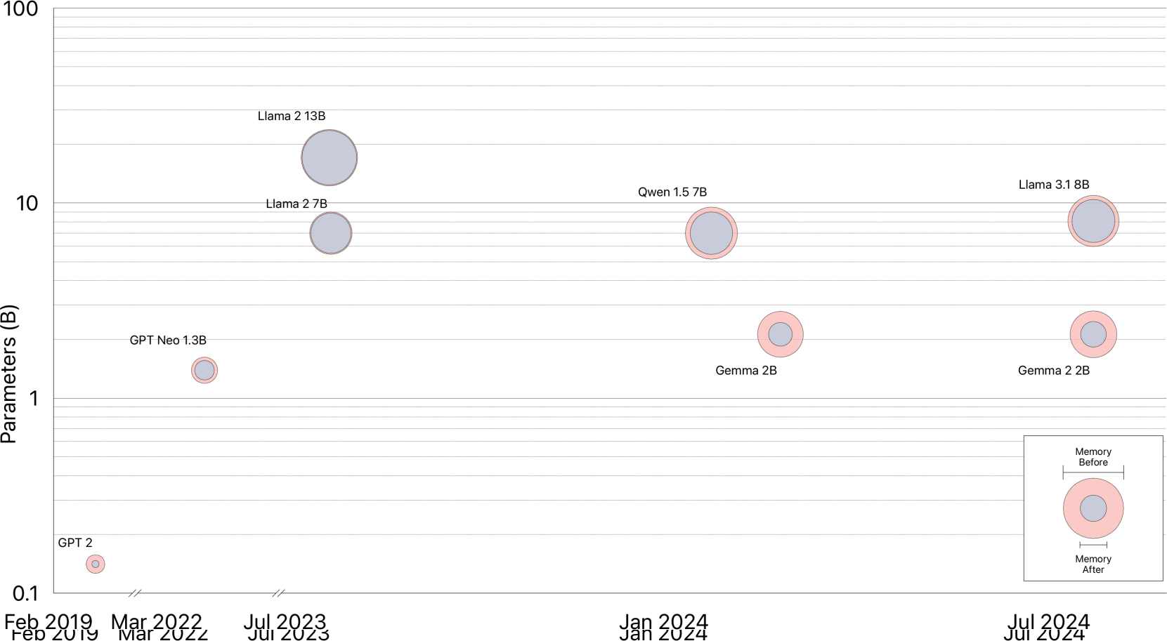
🔼 This figure shows the memory usage and maximum attainable batch size for various language models when using the Cut Cross-Entropy (CCE) method. It demonstrates that CCE significantly reduces the memory footprint of the loss computation, thereby enabling the use of larger batch sizes without sacrificing training speed or convergence. The chart visually compares CCE’s performance to regular cross-entropy, showcasing the dramatic reduction in memory consumption achieved by CCE.
read the caption
(b) Cut cross-entropy (ours)

🔼 Figure 1 is a comparison of memory usage and maximum batch size for various large language models (LLMs) under two different cross-entropy loss implementations: regular cross-entropy and the authors’ proposed Cut Cross-Entropy (CCE). The models are trained using a 16-GPU setup with fully-sharded data parallelism, activation checkpointing, and a mixed-precision AdamW optimizer. The figure shows that the memory consumption of the cross-entropy loss is significantly reduced by CCE. This allows for a substantial increase in the maximum batch size attainable during training (ranging from 1.5x to 10x), without affecting training speed or convergence. Memory usage is broken down by component (weights, optimizer states, activations, and log-probabilities). Table A3 provides more details on the exact memory usage numbers.
read the caption
Figure 1: Memory use and maximum attainable batch size (in millions of tokens) for a variety of frontier models on a 16-GPU (80 GB each) fully-sharded data-parallel setup (Rajbhandari et al., 2020) with activation checkpointing (Chen et al., 2016) and a mixed-precision 16-bit (fp16/bf16) AdamW optimizer (Kingma & Ba, 2015; Loshchilov & Hutter, 2019). For each model, we break its memory use down into weights and optimizer states, activation checkpoints, and the log-probabilities computed by the cross-entropy loss layer. Our Cut Cross-Entropy (CCE) enables increasing the batch size by 1.5x (Llama 2 13B) to 10x (GPT 2, Gemma 2 2B), with no sacrifice in speed or convergence. Exact values in Table A3.

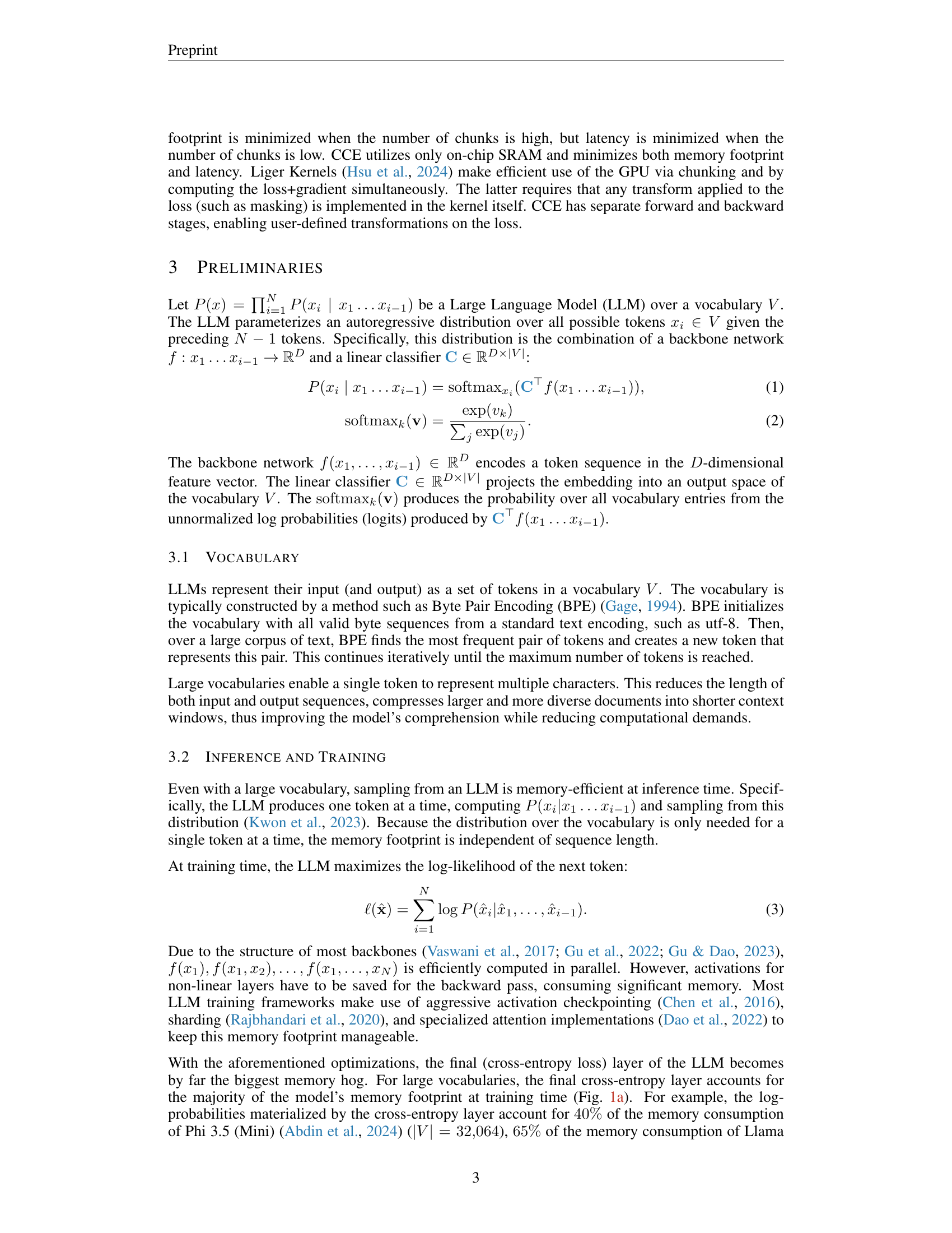
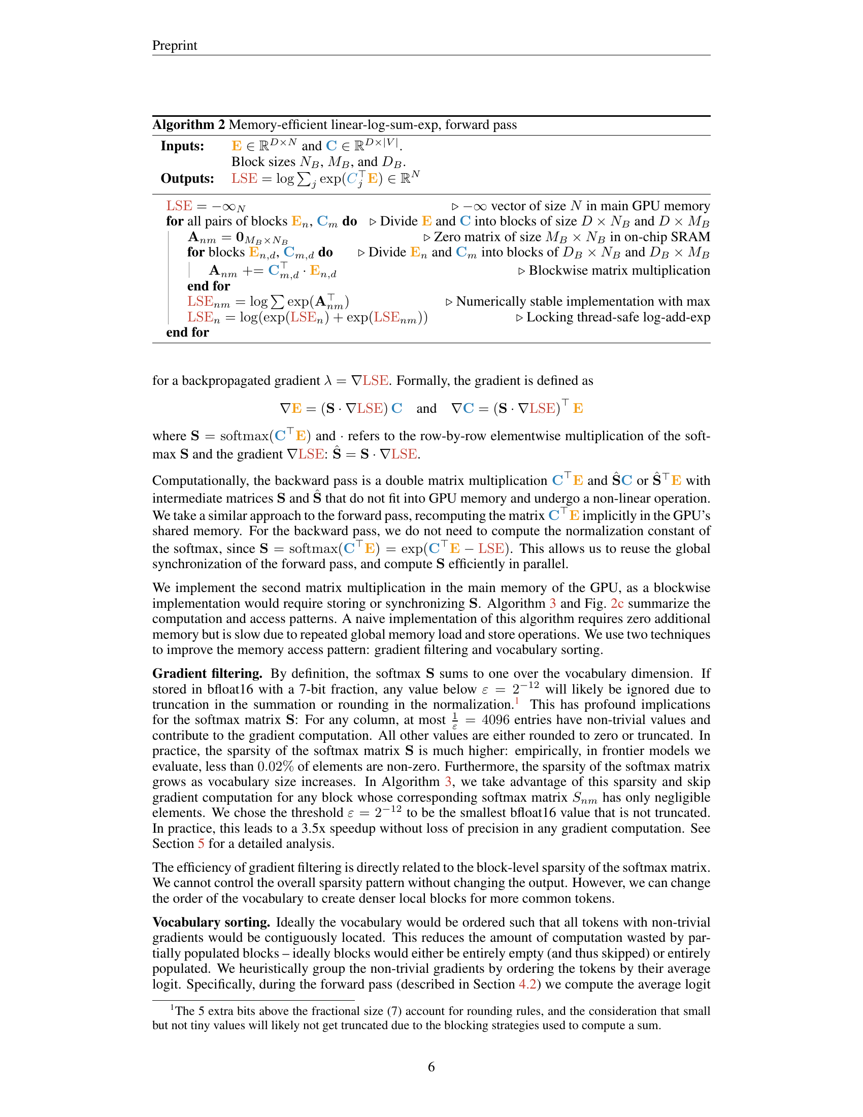
🔼 This figure illustrates the access patterns and computation involved in the indexed matrix multiplication during the forward pass of the Cut Cross-Entropy (CCE) algorithm. It’s a block diagram showing how the algorithm efficiently computes the dot product between network embeddings and classifier weights without materializing the entire logit matrix in global memory. The inputs, including embeddings (E) and classifier weights (C), are divided into blocks, and the operations are performed blockwise to leverage GPU cache efficiently. The result of the indexed matrix multiplication is written to global memory.
read the caption
(a) Indexed matmul (forward)

🔼 This figure shows the forward pass of the linear-log-sum-exp operation used in the Cut Cross-Entropy (CCE) method. The linear-log-sum-exp computation is a crucial part of calculating the cross-entropy loss efficiently in CCE. The diagram illustrates the process of computing the log-sum-exp (LSE) values, which involves intermediate matrix multiplications and reduction operations performed on smaller blocks to optimize memory usage. The specific access patterns and computations are shown to highlight the efficiency of this approach.
read the caption
(b) Linear-log-sum-exp, forward pass

🔼 This figure shows the backward pass of the linear-log-sum-exp operation. The backward pass is crucial for calculating gradients during training, allowing the model to adjust its weights and improve its accuracy. The illustration details the computational steps and memory access patterns involved in this process, highlighting the efficiency and memory savings achieved by the proposed Cut Cross-Entropy (CCE) method. It shows how the CCE method efficiently handles large vocabularies while keeping memory consumption low.
read the caption
(c) Linear-log-sum-exp, backward pass

🔼 Figure 2 illustrates the computational steps and memory access patterns of three key operations within the Cut Cross-Entropy (CCE) method. Panel (a) shows the blockwise indexed matrix multiplication, which efficiently computes the dot product of the classifier weights and embeddings, avoiding the need to store the entire logit matrix. This is followed by (b) the linear-log-sum-exp forward pass, illustrating how the log-sum-exp operation is performed efficiently in a blockwise manner to prevent memory overflow. Finally, (c) displays the corresponding backward pass, outlining how gradients are calculated efficiently using the same blockwise approach. Algorithms 1, 2, and 3 in the paper provide detailed pseudocode for each of these operations.
read the caption
Figure 2: Access patterns and computation of blockwise (a) indexed matrix multiplication, (b) linear-log-sum-exp forward pass, and (c) linear-log-sum-exp backward pass. See Algorithms 1, 2 and 3 for the corresponding algorithms.

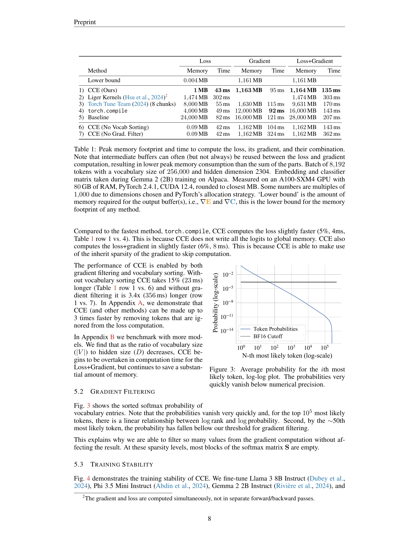
🔼 This log-log plot displays the average probability of the i-th most likely token in the vocabulary. The y-axis represents the probability (on a logarithmic scale), and the x-axis represents the rank (also on a logarithmic scale). The graph shows how rapidly the probabilities decrease as the token rank increases. This demonstrates that the probabilities for many less frequent tokens fall below the level of numerical precision, which has implications for memory efficiency in computing cross-entropy loss, as detailed in the paper.
read the caption
Figure 3: Average probability for the i𝑖iitalic_ith most likely token, log-log plot. The probabilities very quickly vanish below numerical precision.

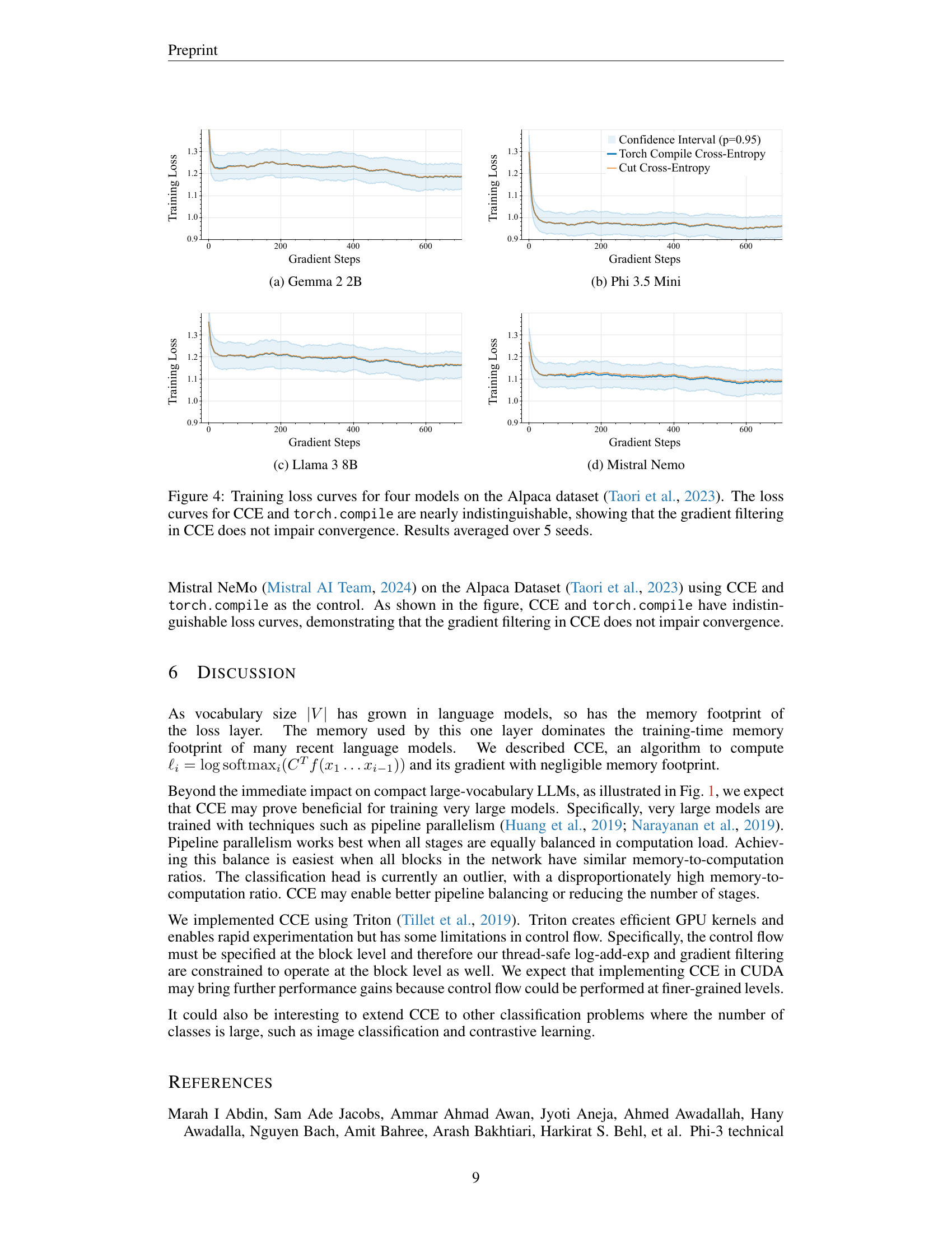
🔼 The figure shows training loss curves for the Gemma 2 2B model, comparing the performance of Cut Cross-Entropy (CCE) and Torch Compile Cross-Entropy. Both methods exhibit nearly identical loss curves over the course of training, indicating that CCE’s gradient filtering does not negatively impact convergence. The graph plots training loss against the number of gradient steps. Confidence intervals are shown to illustrate the variability across multiple training runs.
read the caption
(a) Gemma 2 2B

🔼 This figure displays the training loss curves for the Phi 3.5 Mini language model. The curves compare the performance of Cut Cross-Entropy (CCE) against a baseline method (torch.compile). The near-identical curves demonstrate that CCE’s gradient filtering technique does not negatively impact the model’s convergence during training. Results are averaged over five separate training runs (seeds) for a more robust comparison.
read the caption
(b) Phi 3.5 Mini
More on tables
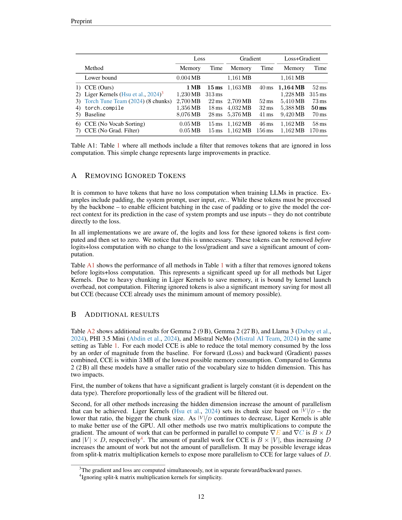
🔼 Table A1 presents a revised version of Table 1, incorporating a filter that excludes tokens not contributing to the loss calculation (e.g., padding tokens). This simple modification significantly improves the efficiency of all the methods evaluated, as shown by the runtime and memory consumption data. The table provides a direct comparison of various cross-entropy loss computation methods, highlighting how effectively this pre-processing step reduces the memory footprint and computation time for each.
read the caption
Table A1: Table 1 where all methods include a filter that removes tokens that are ignored in loss computation. This simple change represents large improvements in practice.
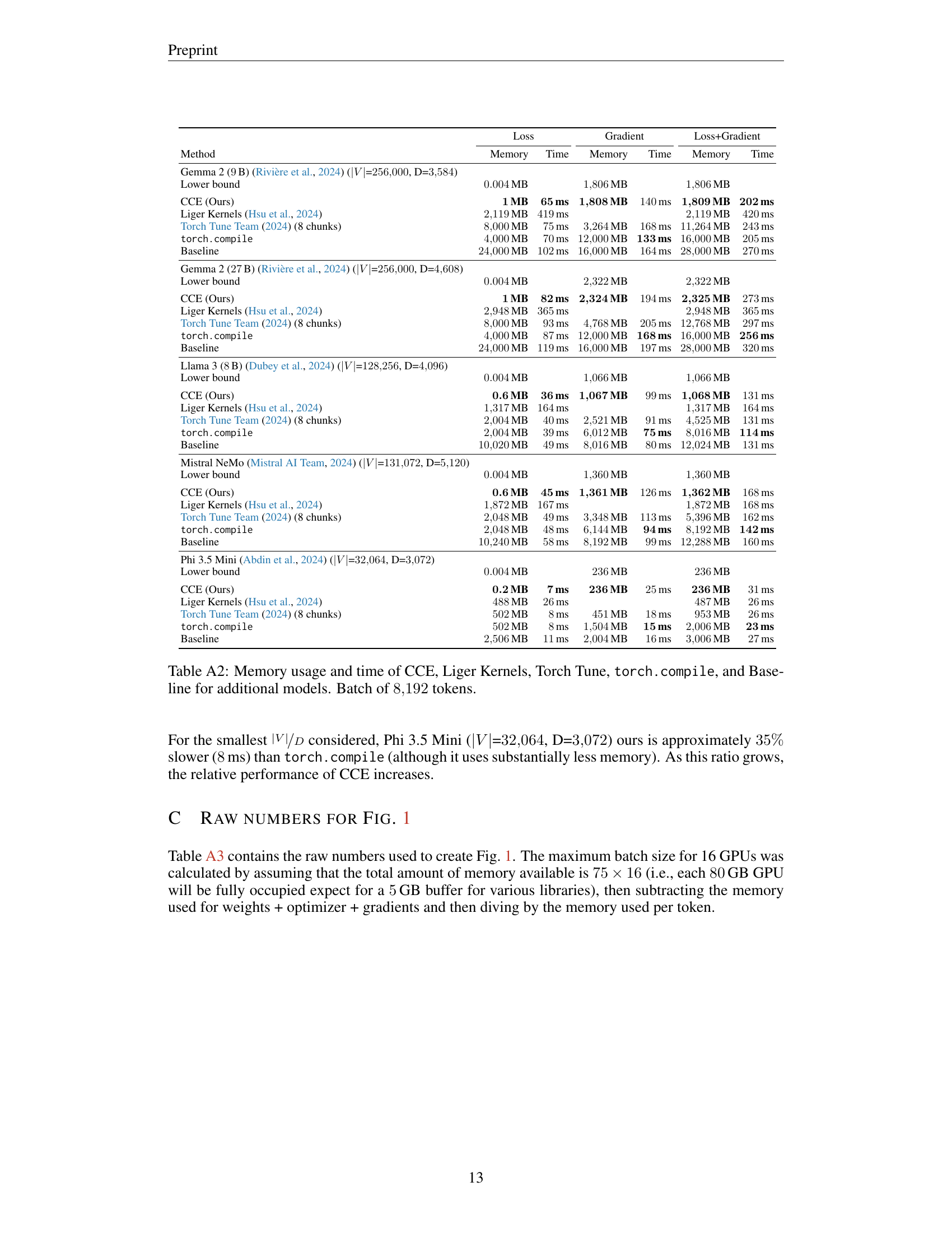
🔼 This table presents a comparison of the memory usage and runtime performance of different cross-entropy loss computation methods across various large language models. The methods compared are Cut Cross-Entropy (CCE), Liger Kernels, Torch Tune, Torch Compile, and a baseline PyTorch implementation. The models used include Gemma 2 (9B, 27B), Llama 3 (8B), Mistral NeMo, and Phi 3.5 Mini. The experiment uses a batch size of 8,192 tokens for each model. For each method and model, the table shows the memory usage for loss computation, gradient calculation, and both together, along with the corresponding computation times. The results highlight CCE’s superior memory efficiency compared to other methods, demonstrating significant reductions in memory consumption while maintaining competitive runtime performance.
read the caption
Table A2: Memory usage and time of CCE, Liger Kernels, Torch Tune, torch.compile, and Baseline for additional models. Batch of 8192819281928192 tokens.
| Method | Loss Memory | Loss Time | Gradient Memory | Gradient Time | Loss+Gradient Memory | Loss+Gradient Time |
|---|---|---|---|---|---|---|
| Lower bound | 0.004MB | 1161MB | 1161MB | |||
| 1) CCE (Ours) | 1MB | 43ms | 1163MB | 95ms | 1164MB | 135ms |
| 2) Liger Kernels (Hsu et al., 2024)2 | 1474MB | 302ms | 1474MB | 303ms | ||
| 3) Torch Tune Team (2024) (8 chunks) | 8000MB | 55ms | 1630MB | 115ms | 9631MB | 170ms |
4) torch.compile | 4000MB | 49ms | 12000MB | 92ms | 16000MB | 143ms |
| 5) Baseline | 24000MB | 82ms | 16000MB | 121ms | 28000MB | 207ms |
| 6) CCE (No Vocab Sorting) | 0.09MB | 42ms | 1162MB | 104ms | 1162MB | 143ms |
| 7) CCE (No Grad. Filter) | 0.09MB | 42ms | 1162MB | 324ms | 1162MB | 362ms |
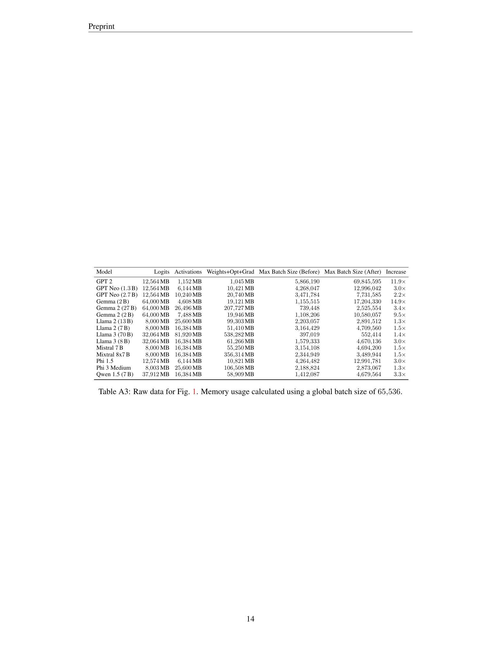
🔼 This table provides the raw data used to generate Figure 1 in the paper. It details the memory usage breakdown for various large language models (LLMs), categorized into log probabilities, activations, and weights/optimizer/gradients. The memory usage is calculated using a global batch size of 65,536 tokens. For each model, the table shows the maximum batch size attainable before and after applying the Cut Cross-Entropy (CCE) optimization, along with the resulting increase in batch size.
read the caption
Table A3: Raw data for Fig. 1. Memory usage calculated using a global batch size of 65536655366553665536.
Full paper#
