↗ arXiv ↗ Hugging Face ↗ Papers with Code
TL;DR#
Deploying large multimodal language models (MLLMs) on mobile phones is hindered by limitations in memory and processing power. Existing solutions often struggle with slow speeds and high resource consumption, limiting their practicality for real-time applications. This is a critical issue because mobile phones offer a seamless platform for integrating MLLMs into everyday tasks.
This paper introduces BlueLM-V-3B, which tackles these challenges via a novel co-design strategy. This involves optimizing the model’s architecture for smaller size and faster inference, as well as implementing system optimizations tailored for mobile hardware. BlueLM-V-3B achieves a generation speed of 24.4 tokens/s on a MediaTek Dimensity 9300 processor and attains the highest average score among comparable models on the OpenCompass benchmark. The results demonstrate a significant step toward making MLLMs more readily available and usable on mobile platforms.
Key Takeaways#
Why does it matter?#
This paper is important because it presents BlueLM-V-3B, a significant advancement in deploying large multimodal language models (MLLMs) on mobile devices. It directly addresses the challenges of limited memory and computational power on mobile phones by using a co-design approach that optimizes both algorithms and system architecture. This work opens new avenues for research on efficient on-device AI and expands the potential applications of MLLMs in mobile environments, impacting areas such as real-time translation and augmented reality.
Visual Insights#

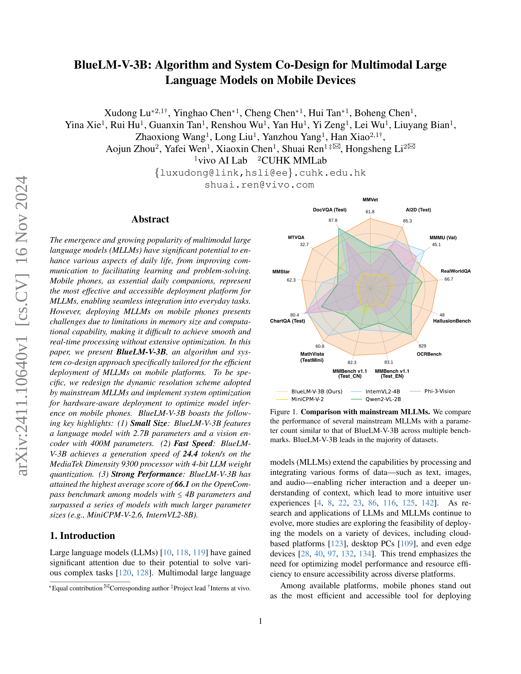
🔼 This figure presents a comparison of BlueLM-V-3B’s performance against other mainstream multimodal large language models (MLLMs) on various benchmark datasets. The models selected for comparison have a similar parameter count to BlueLM-V-3B, ensuring a fair comparison based on model size. The benchmarks assess the MLLMs’ capabilities across a variety of tasks, and the radar chart visually represents the performance of each model on each benchmark. The key takeaway is that BlueLM-V-3B outperforms most of the other models in a majority of the benchmark datasets.
read the caption
Figure 1: Comparison with mainstream MLLMs. We compare the performance of several mainstream MLLMs with a parameter count similar to that of BlueLM-V-3B across multiple benchmarks. BlueLM-V-3B leads in the majority of datasets.
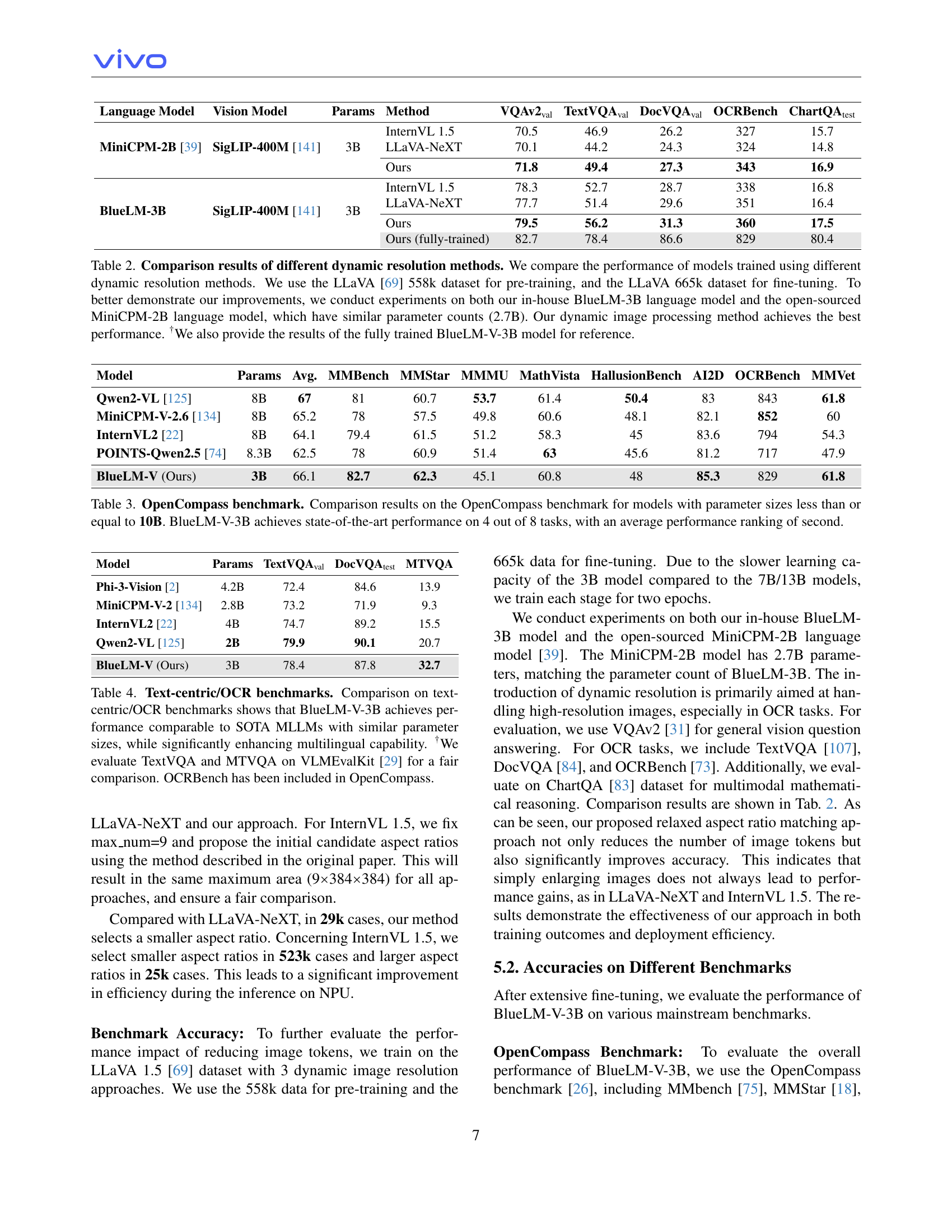
| Type | Public (M) | In-House (M) | In-House / Public |
|---|---|---|---|
| Pure Text | 2.2 | 64.7 | 29.4 |
| Caption | 10.0 | 306.3 | 30.6 |
| VQA | 20.3 | 44.4 | 2.2 |
| OCR | 23.3 | 173.9 | 7.5 |
| Total | 55.8 | 589.3 | 10.6 |
🔼 This table presents a detailed breakdown of the dataset used for the fine-tuning stage of the BlueLM-V-3B model. It includes the number of data points (in millions) for each category (Pure Text, Caption, VQA, OCR) and specifies whether the data originates from publicly available sources or internal (in-house) collections. The in-house/public ratio is also provided for each category, offering insights into the composition of the training data.
read the caption
Table 1: Detailed statistics of the fine-tuning dataset. Summary of dataset types, counts (in millions), and in-house/public ratios for each category used in fine-tuning.
In-depth insights#
Mobile MLLM Design#
Designing Mobile MLLMs presents unique challenges due to limited computational resources and memory constraints of mobile devices. Effective mobile MLLM design necessitates a multi-pronged approach encompassing model compression techniques, such as quantization and pruning, to reduce model size and improve inference speed. Efficient architectures are crucial, potentially employing lightweight models or specialized designs for mobile hardware. Furthermore, system-level optimizations are key, including efficient memory management, optimized data transfer between CPU/GPU/NPU, and hardware-aware parallelization strategies. Addressing the dynamic resolution problem in image processing within MLLMs is vital for both accuracy and efficiency on mobile devices. A successful design will balance model performance, speed, and resource usage, ensuring a smooth user experience in real-world mobile applications. Algorithm and system co-design becomes essential to achieve the best possible results.
Dynamic Resolution#
Dynamic resolution in large language models (LLMs) aims to optimize processing of high-resolution images by adapting the resolution to the model’s needs, thereby improving efficiency and reducing computational demands. However, naive implementations can lead to excessive image enlargement, resulting in a significant increase in image tokens and consequently, slower processing. The paper highlights the problem of exaggerated image enlargement in existing methods and proposes a relaxed aspect ratio matching method. This improved approach reduces the number of image tokens without sacrificing accuracy by strategically selecting resolutions, preventing unnecessary upscaling and improving deployment efficiency on mobile devices. Careful system design, including batched image encoding and pipeline parallelism, further accelerates the image processing, making real-time performance on mobile phones feasible. The overall approach emphasizes algorithm-system co-design, showing that effective optimization needs to go beyond algorithmic improvements and consider the specific constraints and capabilities of the target hardware.
System Optimization#
Optimizing system performance for mobile deployment of large multimodal language models (MLLMs) is crucial due to resource constraints. Hardware-aware optimization is key, focusing on efficient utilization of the mobile Neural Processing Unit (NPU). This involves techniques like mixed-precision quantization (INT4/INT8 for weights and INT16/FP16 for activations) to minimize memory footprint and accelerate computation. Pipeline parallelism and batched processing of image patches further enhance efficiency during image encoding. Addressing the limitations of NPUs in handling long sequences, techniques like token downsampling reduce the number of tokens processed, thereby improving overall speed. Careful framework design, including decoupling image encoding from instruction processing, and implementing chunked computation for input tokens, contributes significantly to the overall efficiency. These strategies, when combined, enable real-time performance of complex MLLMs on resource-constrained mobile devices. Efficient memory management is implicitly addressed to prevent memory issues and ensure seamless operation.
Benchmark Results#
A thorough analysis of benchmark results in a research paper requires a multi-faceted approach. First, identify the specific benchmarks used; understanding their strengths and limitations is crucial for interpreting the results. Next, examine the metrics reported; are they appropriate for the task and model type? Consider the scale of the benchmarks: larger, more diverse datasets generally lead to more robust evaluations. Analyze the performance relative to baselines and state-of-the-art models: how significant is the improvement? Statistical significance is key: mere performance gains are not enough; results should be backed by statistical testing. Pay close attention to any error bars or confidence intervals presented to assess the reliability of the findings. Finally, consider potential biases or limitations: were any specific conditions favorable to a particular model, and does this impact the overall generalizability? A well-written benchmark analysis section will address all of these points, providing a clear, unbiased assessment of the model’s performance.
Future Work#
The paper’s ‘Future Work’ section could explore several promising avenues. Extending BlueLM-V-3B’s multilingual capabilities is crucial, given its current strong but not exhaustive performance. Further research into optimizing the model for a wider range of mobile devices with varying processing power and memory is essential to maximize accessibility. Investigating more sophisticated training techniques including advanced quantization methods or novel architectures to further enhance efficiency and performance is another important area. Finally, exploring different deployment strategies, such as edge computing or model compression, could significantly improve the real-time response and user experience. A detailed analysis of potential failure modes and robustness testing would also solidify the model’s reliability and pave the way for wider adoption.
More visual insights#
More on figures

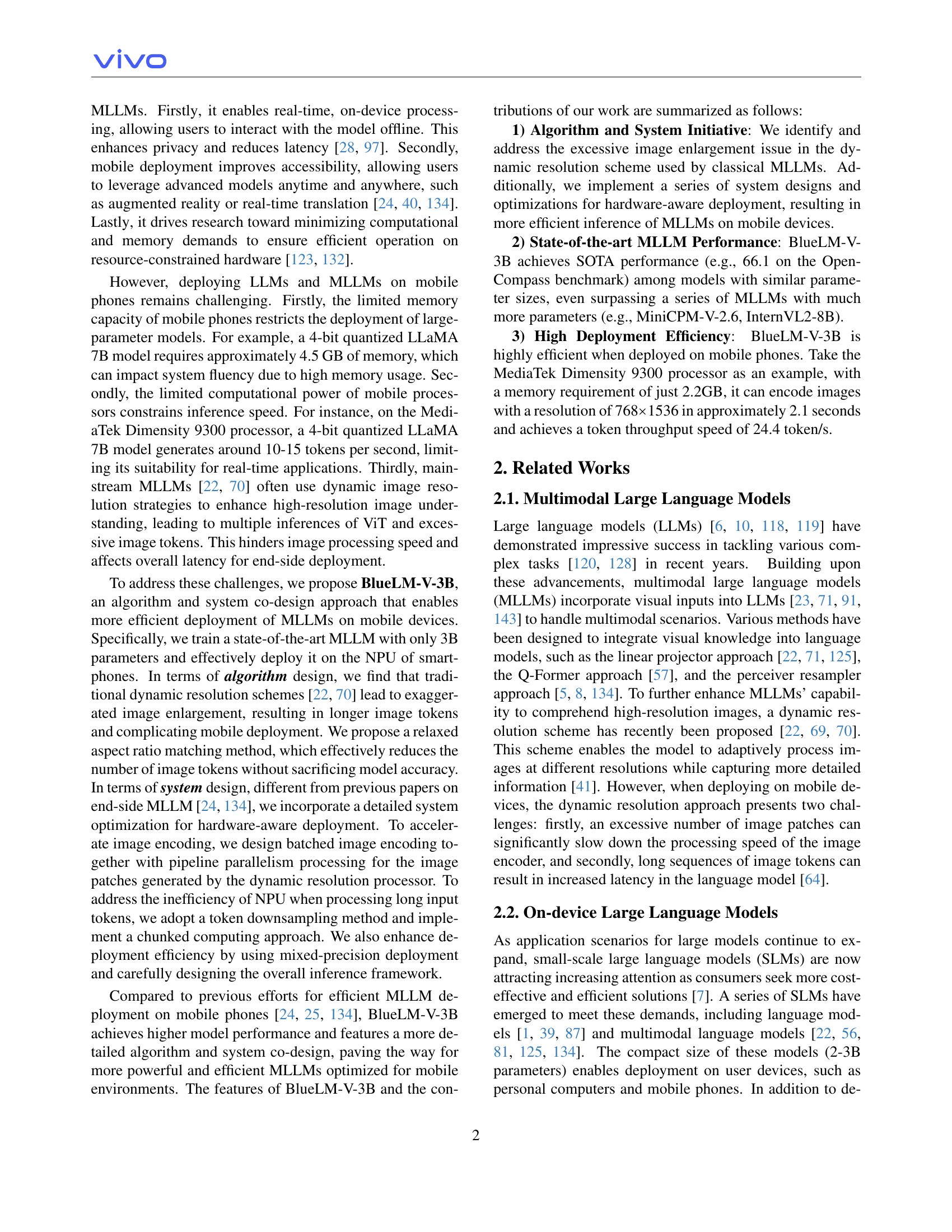
🔼 BlueLM-V-3B’s architecture is a modified version of the LLaVA approach. It consists of an image encoder (SigLIP-400M), an MLP projector, and a language model (BlueLM-2.7B). To handle high-resolution images efficiently, a dynamic resolution processing module is included, similar to those used in LLaVA-NeXT and InternVL 1.5. A token downsampler is added to reduce the number of tokens, which improves efficiency for mobile devices. The diagram shows how images and text are processed and passed to the language model for response generation.
read the caption
Figure 2: Model architecture of BlueLM-V-3B. The architecture of BlueLM-V-3B follows the classical LLaVA approach. We integrate a dynamic resolution processing module (as in LLaVA-NeXT [70] and InternVL 1.5 [22]) to enhance model capabilities and apply token downsampling to reduce deployment complexity.

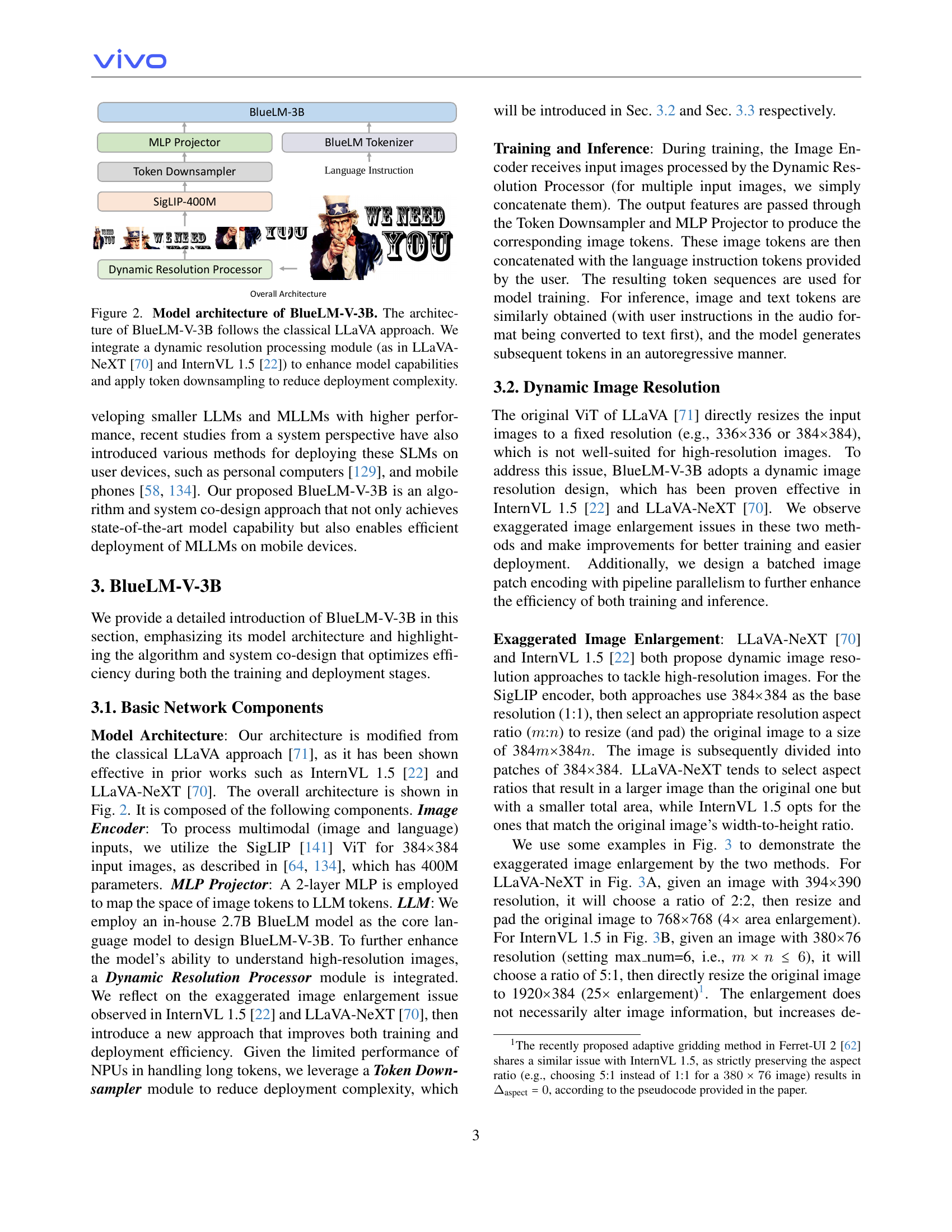
🔼 This figure compares the image processing approaches of three different Multimodal Large Language Models (MLLMs): LLaVA-NeXT, InternVL 1.5, and the authors’ proposed BlueLM-V-3B. It highlights how each model handles high-resolution images. LLaVA-NeXT and InternVL 1.5 both utilize dynamic resolution schemes but tend to significantly enlarge images, leading to a larger number of image tokens after processing by the Vision Transformer (ViT). LLaVA-NeXT increases the image area by 4 times, while InternVL 1.5 increases it by 25 times. In contrast, BlueLM-V-3B uses a fixed 1:1 aspect ratio, minimizing image enlargement and resulting in the fewest image tokens. This optimized approach leads to more efficient model training and deployment on mobile devices.
read the caption
Figure 3: Existing methods overly enlarge images. (A) For LLaVA-NeXT, an image with resolution 394×\times×390 selects a 2:2 aspect ratio and is resized and padded to 768×\times×768 (4×\times× area enlargement). (B) For InternVL 1.5, an image with resolution 380×\times×76 chooses a 5:1 aspect ratio and is directly resized to 1920×\times×384 (25×\times× area enlargement). BlueLM-V-3B, in contrast, selects a 1:1 aspect ratio for both resolutions, resulting in the minimum number of image tokens after ViT encoding, which can facilitate both model training and deployment.

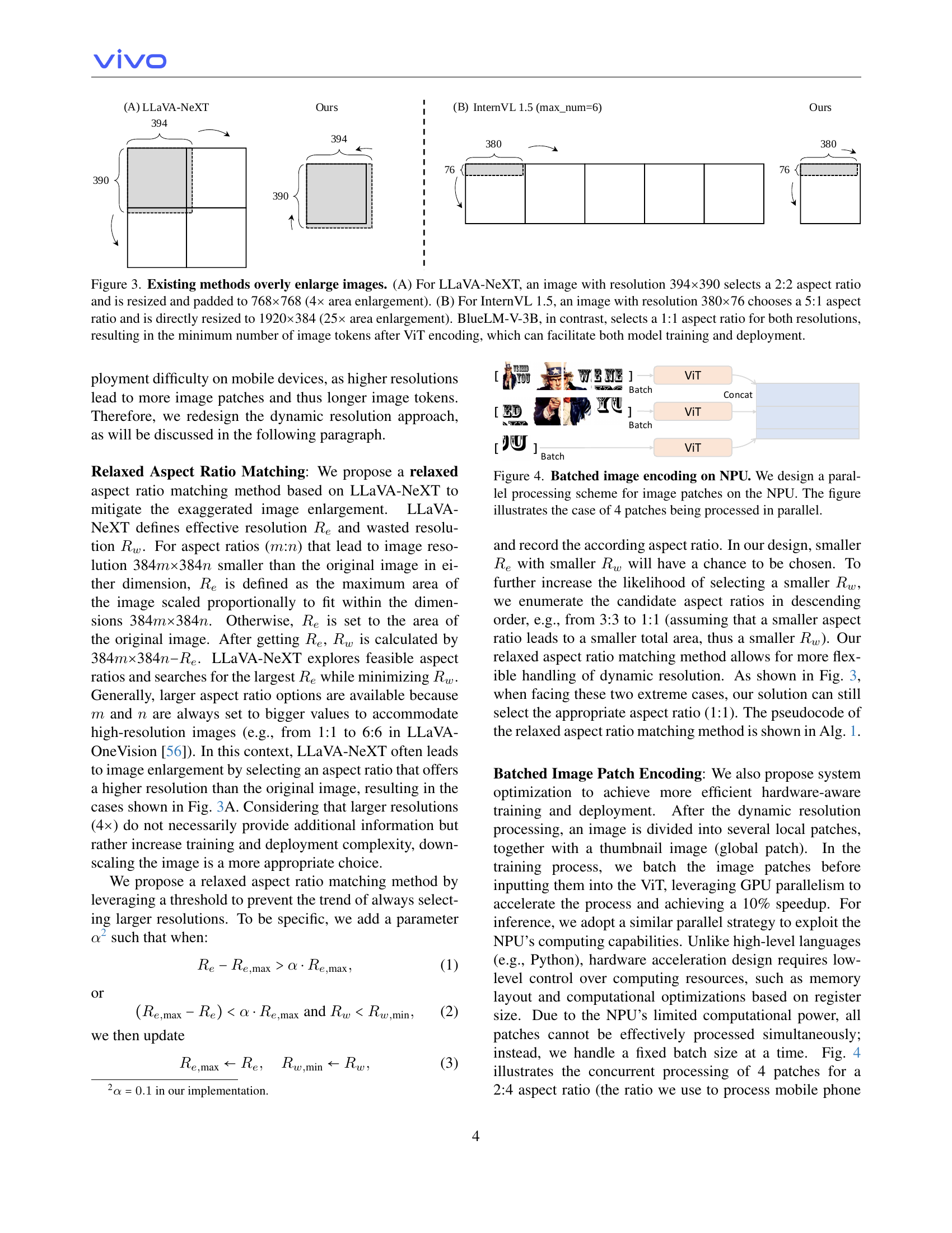
🔼 This figure illustrates the parallel processing of image patches on the Neural Processing Unit (NPU) of a mobile device, a key optimization in BlueLM-V-3B. The image shows four patches being processed concurrently using the batched image encoding approach, significantly improving processing speed. This contrasts with sequential processing of patches, which would be much slower. The system utilizes a pipeline to take advantage of the NPU’s capabilities and minimize latency.
read the caption
Figure 4: Batched image encoding on NPU. We design a parallel processing scheme for image patches on the NPU. The figure illustrates the case of 4 patches being processed in parallel.

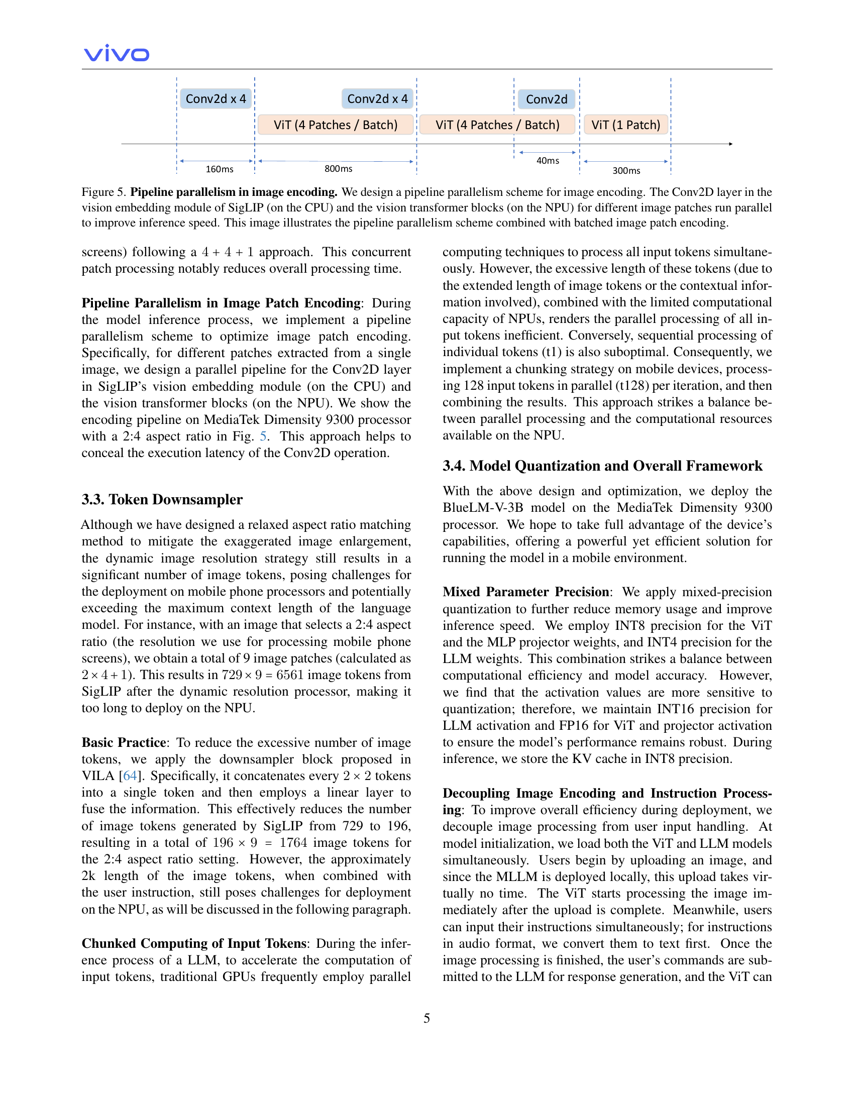
🔼 This figure illustrates how pipeline parallelism and batched image encoding are used in BlueLM-V-3B to speed up image processing. The process begins with multiple image patches from a single image, which are encoded in parallel using the Conv2D layer of SigLIP on the CPU. These intermediate results then feed into the Vision Transformer blocks on the NPU for further parallel processing, significantly shortening the overall inference time.
read the caption
Figure 5: Pipeline parallelism in image encoding. We design a pipeline parallelism scheme for image encoding. The Conv2D layer in the vision embedding module of SigLIP (on the CPU) and the vision transformer blocks (on the NPU) for different image patches run parallel to improve inference speed. This image illustrates the pipeline parallelism scheme combined with batched image patch encoding.

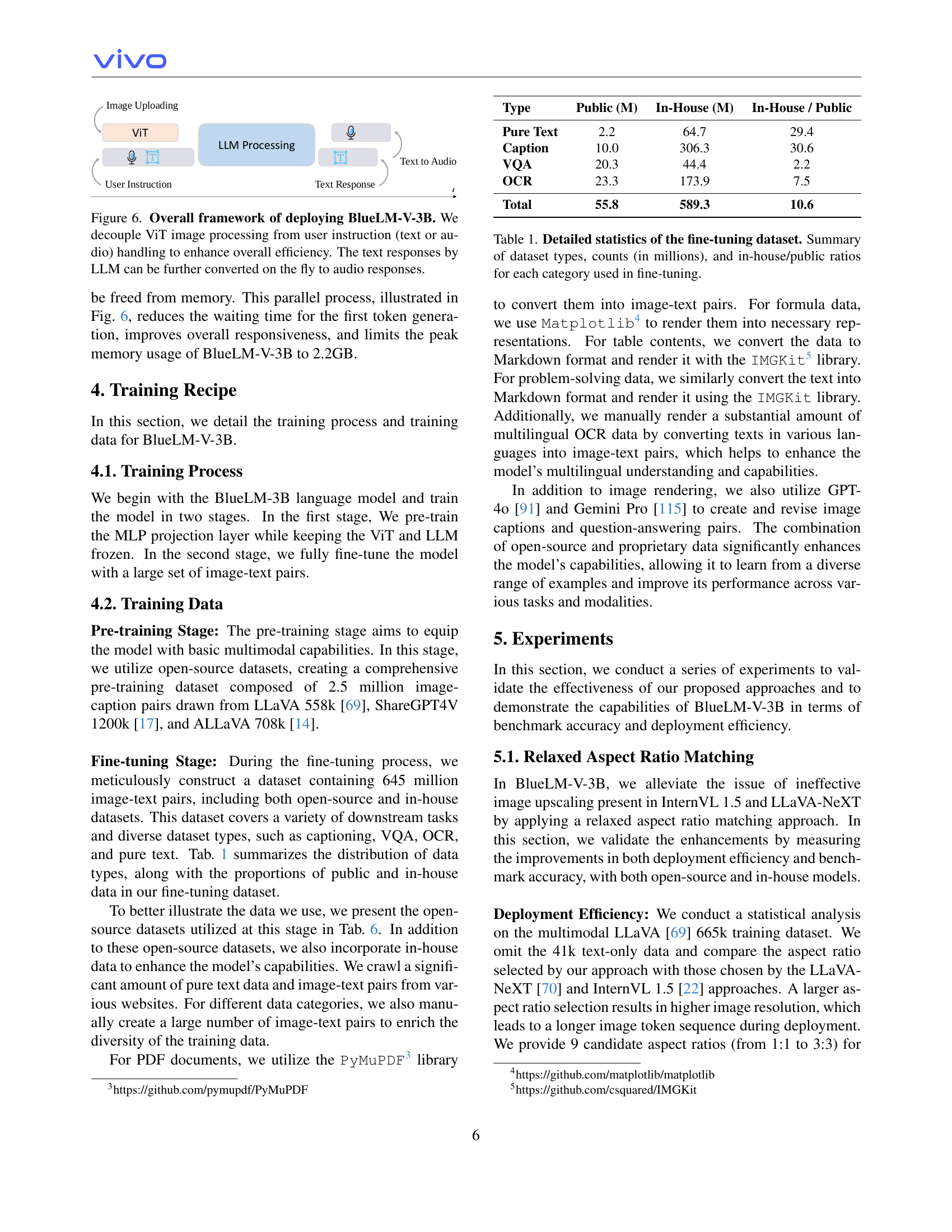
🔼 The figure illustrates the overall framework of the BlueLM-V-3B deployment. It highlights a key efficiency improvement: decoupling the image processing (handled by the ViT) from user input processing (text or audio instructions). This allows parallel processing, where image encoding happens concurrently with the handling of user instructions. Once the image encoding is finished, the user instruction is submitted to the LLM for response generation. For added user-friendliness, the generated text responses can be converted into audio responses in real-time.
read the caption
Figure 6: Overall framework of deploying BlueLM-V-3B. We decouple ViT image processing from user instruction (text or audio) handling to enhance overall efficiency. The text responses by LLM can be further converted on the fly to audio responses.

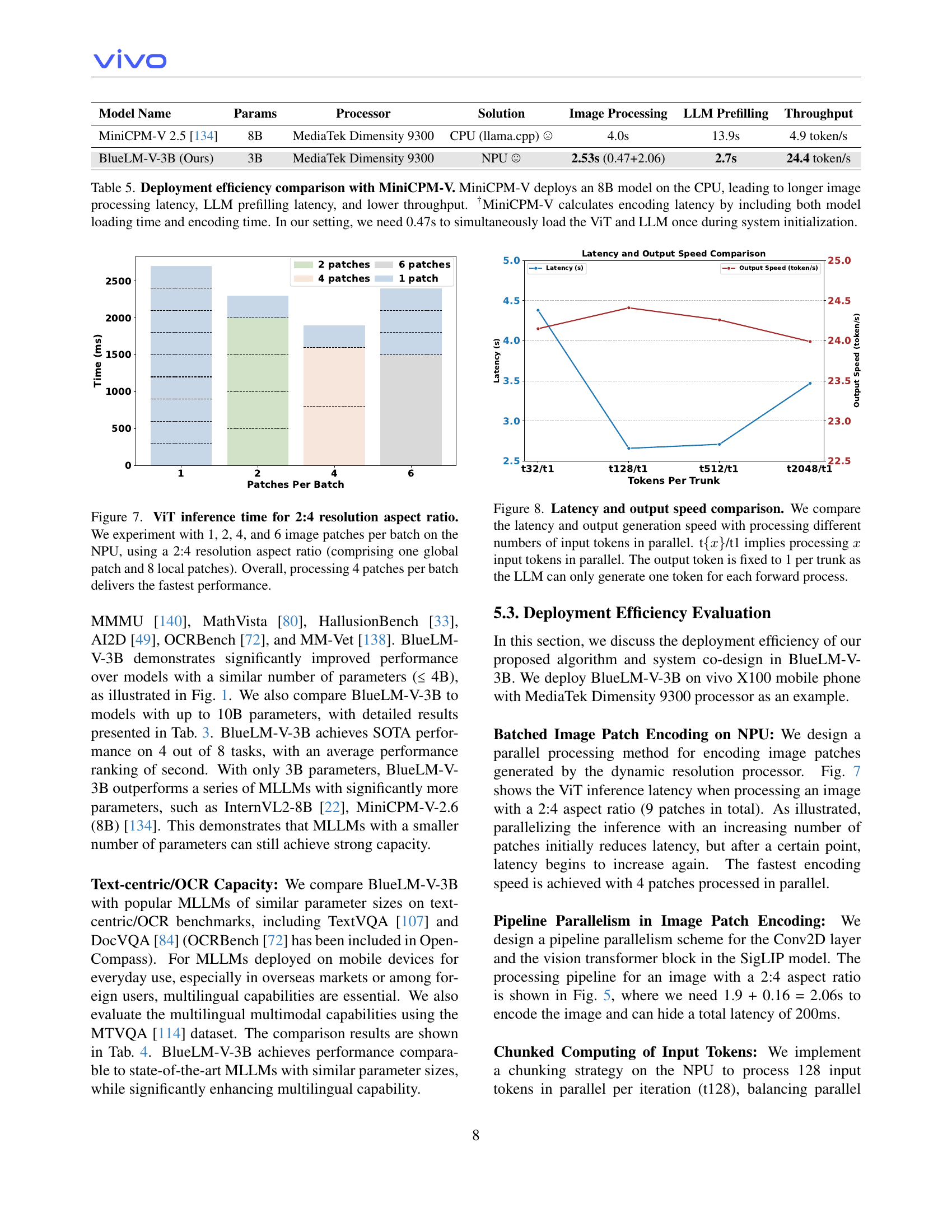
🔼 This figure shows the inference time of the Vision Transformer (ViT) model when processing image patches with a 2:4 aspect ratio. The experiment varies the number of image patches processed per batch on the Neural Processing Unit (NPU): 1, 2, 4, and 6. Each batch consists of a global patch and 8 local patches. The results show that processing 4 patches per batch achieves the fastest inference time, indicating an optimal balance between parallelization and computational overhead.
read the caption
Figure 7: ViT inference time for 2:4 resolution aspect ratio. We experiment with 1, 2, 4, and 6 image patches per batch on the NPU, using a 2:4 resolution aspect ratio (comprising one global patch and 8 local patches). Overall, processing 4 patches per batch delivers the fastest performance.

🔼 Figure 8 illustrates the trade-off between latency and throughput when processing various numbers of input tokens concurrently in the BlueLM-V-3B model. The x-axis represents the number of tokens processed in parallel (t{x}/t1 denotes processing x tokens in parallel), while the y-axis shows both latency (in seconds) and output speed (in tokens per second). The figure highlights that increasing the number of parallel tokens initially reduces latency and increases throughput, but beyond a certain point, this trend reverses likely due to the limitations of NPU resources. The output token count remains fixed at one per forward pass, independent of the number of parallel tokens processed, reflecting the autoregressive nature of the LLM. This emphasizes the efficiency optimization achieved in BlueLM-V-3B.
read the caption
Figure 8: Latency and output speed comparison. We compare the latency and output generation speed with processing different numbers of input tokens in parallel. t{x𝑥xitalic_x}/t1 implies processing x𝑥xitalic_x input tokens in parallel. The output token is fixed to 1 per trunk as the LLM can only generate one token for each forward process.

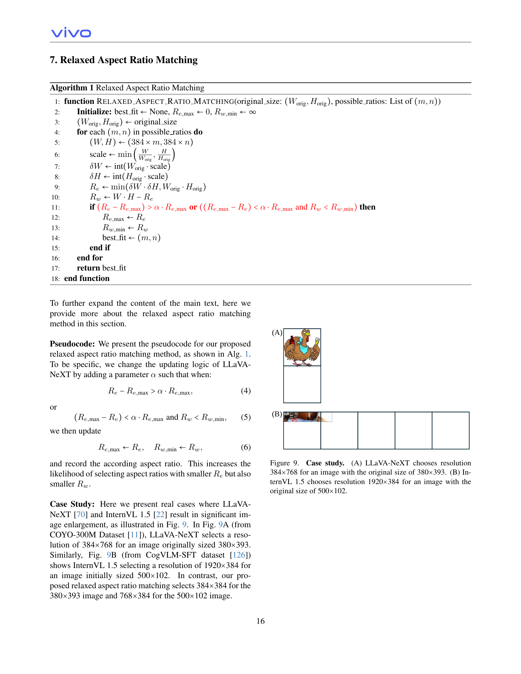
🔼 This figure demonstrates the exaggerated image resolution in existing methods. Panel (A) shows that LLaVA-NeXT chooses a resolution of 384x768 for an image originally sized 380x393, significantly increasing the image size. Panel (B) illustrates InternVL 1.5 selecting a resolution of 1920x384 for an image initially sized 500x102, further highlighting the issue of excessive enlargement. This excessive enlargement increases the number of image tokens, hindering efficient deployment on mobile devices.
read the caption
Figure 9: Case study. (A) LLaVA-NeXT chooses resolution 384×\times×768 for an image with the original size of 380×\times×393. (B) InternVL 1.5 chooses resolution 1920×\times×384 for an image with the original size of 500×\times×102.
More on tables
| Language Model | Vision Model | Params | Method | VQAv2val | TextVQAval | DocVQAval | OCRBench | ChartQAtest |
|---|---|---|---|---|---|---|---|---|
| MiniCPM-2B [39] | SigLIP-400M [141] | 3B | InternVL 1.5 | 70.5 | 46.9 | 26.2 | 327 | 15.7 |
| LLaVA-NeXT | 70.1 | 44.2 | 24.3 | 324 | 14.8 | |||
| Ours | 71.8 | 49.4 | 27.3 | 343 | 16.9 | |||
| BlueLM-3B | SigLIP-400M [141] | 3B | InternVL 1.5 | 78.3 | 52.7 | 28.7 | 338 | 16.8 |
| LLaVA-NeXT | 77.7 | 51.4 | 29.6 | 351 | 16.4 | |||
| Ours | 79.5 | 56.2 | 31.3 | 360 | 17.5 | |||
| Ours (fully-trained) | 82.7 | 78.4 | 86.6 | 829 | 80.4 |
🔼 This table compares the performance of different dynamic image resolution methods used in training multimodal large language models (MLLMs). The comparison uses two models with similar parameter counts: the in-house BlueLM-3B and the open-source MiniCPM-2B (both around 2.7B parameters). The LLaVA dataset (558k for pre-training and 665k for fine-tuning) was used for training. The table highlights the superior performance of the proposed dynamic image processing method in BlueLM-V-3B, and also includes results for a fully trained BlueLM-V-3B model for additional context.
read the caption
Table 2: Comparison results of different dynamic resolution methods. We compare the performance of models trained using different dynamic resolution methods. We use the LLaVA [69] 558k dataset for pre-training, and the LLaVA 665k dataset for fine-tuning. To better demonstrate our improvements, we conduct experiments on both our in-house BlueLM-3B language model and the open-sourced MiniCPM-2B language model, which have similar parameter counts (2.7B). Our dynamic image processing method achieves the best performance. †We also provide the results of the fully trained BlueLM-V-3B model for reference.
| Model | Params | Avg. | MMBench | MMStar | MMMU | MathVista | HallusionBench | AI2D | OCRBench | MMVet |
|---|---|---|---|---|---|---|---|---|---|---|
| Qwen2-VL [125] | 8B | 67 | 81 | 60.7 | 53.7 | 61.4 | 50.4 | 83 | 843 | 61.8 |
| MiniCPM-V-2.6 [134] | 8B | 65.2 | 78 | 57.5 | 49.8 | 60.6 | 48.1 | 82.1 | 852 | 60 |
| InternVL2 [22] | 8B | 64.1 | 79.4 | 61.5 | 51.2 | 58.3 | 45 | 83.6 | 794 | 54.3 |
| POINTS-Qwen2.5 [74] | 8.3B | 62.5 | 78 | 60.9 | 51.4 | 63 | 45.6 | 81.2 | 717 | 47.9 |
| BlueLM-V (Ours) | 3B | 66.1 | 82.7 | 62.3 | 45.1 | 60.8 | 48 | 85.3 | 829 | 61.8 |
🔼 This table presents a comparison of BlueLM-V-3B’s performance against other large language models (LLMs) on the OpenCompass benchmark. OpenCompass is a comprehensive evaluation suite for foundation models, assessing performance across a range of tasks. The table focuses on models with 10 billion parameters or fewer. BlueLM-V-3B, despite having only 3 billion parameters, achieves state-of-the-art results on four out of the eight tasks evaluated and ranks second overall.
read the caption
Table 3: OpenCompass benchmark. Comparison results on the OpenCompass benchmark for models with parameter sizes less than or equal to 10B. BlueLM-V-3B achieves state-of-the-art performance on 4 out of 8 tasks, with an average performance ranking of second.
| Model | Params | TextVQAval | DocVQAtest | MTVQA |
|---|---|---|---|---|
| Phi-3-Vision [2] | 4.2B | 72.4 | 84.6 | 13.9 |
| MiniCPM-V-2 [134] | 2.8B | 73.2 | 71.9 | 9.3 |
| InternVL2 [22] | 4B | 74.7 | 89.2 | 15.5 |
| Qwen2-VL [125] | 2B | 79.9 | 90.1 | 20.7 |
| BlueLM-V (Ours) | 3B | 78.4 | 87.8 | 32.7 |
🔼 Table 4 presents a comparison of BlueLM-V-3B’s performance on text-centric and OCR benchmarks against other state-of-the-art (SOTA) Multimodal Large Language Models (MLLMs). The focus is on models with similar parameter sizes. The results show BlueLM-V-3B achieves comparable performance to these SOTA models but with a significant advantage in multilingual capabilities. To ensure fairness, TextVQA and MTVQA evaluations used the VLMEvalKit [29]. Note that OCRBench results are included within the OpenCompass benchmark.
read the caption
Table 4: Text-centric/OCR benchmarks. Comparison on text-centric/OCR benchmarks shows that BlueLM-V-3B achieves performance comparable to SOTA MLLMs with similar parameter sizes, while significantly enhancing multilingual capability. †We evaluate TextVQA and MTVQA on VLMEvalKit [29] for a fair comparison. OCRBench has been included in OpenCompass.
| Model Name | Params | Processor | Solution | Image Processing | LLM Prefilling | Throughput |
|---|---|---|---|---|---|---|
| MiniCPM-V 2.5 [134] | 8B | MediaTek Dimensity 9300 | CPU (llama.cpp) ☹ | 4.0s | 13.9s | 4.9 token/s |
| BlueLM-V-3B (Ours) | 3B | MediaTek Dimensity 9300 | NPU ☺ | 2.53s (0.47+2.06) | 2.7s | 24.4 token/s |
🔼 This table compares the deployment efficiency of BlueLM-V-3B with MiniCPM-V. MiniCPM-V uses an 8B parameter model and runs on the CPU, resulting in significantly slower image processing, LLM pre-filling (preparing the language model for generation), and overall throughput (tokens generated per second) compared to BlueLM-V-3B. The difference is attributed to MiniCPM-V’s CPU deployment and the inclusion of model loading time in its latency calculation. BlueLM-V-3B’s superior efficiency stems from its smaller 3B parameter model and use of the NPU (Neural Processing Unit). The 0.47s load time for BlueLM-V-3B accounts for the simultaneous loading of both Vision Transformer (ViT) and Language Model (LLM) components at the start of the system initialization.
read the caption
Table 5: Deployment efficiency comparison with MiniCPM-V. MiniCPM-V deploys an 8B model on the CPU, leading to longer image processing latency, LLM prefilling latency, and lower throughput. †MiniCPM-V calculates encoding latency by including both model loading time and encoding time. In our setting, we need 0.47s to simultaneously load the ViT and LLM once during system initialization.
| Task | Dataset |
|---|---|
| Text-only | ALLaVA [14], ScienceQA [79], Orca-Math [90], OpenOrca [63], MetaMathQA [137], WizardLM [130], MathInstruct [117] |
| Caption | TextCaps [104], Screen2Words [122], VizWiz [36], Laion [99], COCO [20], LLaVA [71], ALLaVA [14], SVIT [146], SA1B [51], VSR [66], Chart2Text [48], MultiMath [94], ArXivCap [59], COYO [11] |
| OCR | Wukong [32], HierText [76], TextOCR [108], WildReceipt [111], DocILE [105], SVRD [139], DocLayNet [95], XFUND [131], COCO-Text [121], SROIE [42], FUNSD [44], CORD [92], Paper2Fig100k [98], Docmatix [53], LAION-2B-OCR [65], SynthDoG [50], WebSight [54], DeepForm [112], Kleister [110], TabFact [19] |
| VQA | LVIS-Instruct4V [124], CLEVR [45], TallyQA [3], LNQA [96], Geo170K [102], ALLaVA [14], DocVQA [84], ChartQA [83], ArxivQA [59], GEOS [100], PMC-VQA [144], KVQA [101], Geometry3K [77], MapQA [13], PlotQA [88], ViQuAE [55], VQA-RAD [52], ST-VQA [9], TextVQA [106], LLaVAR [145], SIBR [133], MMC-Inst [68], IconQA [78], GQA [43], SciGraphQA [60], LRV-Instruction [67], DVQA [46], InfographicVQA [85], FigureQA [47], WikiTableQuestions [93], TAT-DQA [147], VisualMRC [113], ScienceQA [79], OCR-VQA [89], WebSRC [21], PathVQA [37], UniGeo [15], ScreenQA [38], VizWiz [35], SVIT [146], CogVLM [126], FM-IQA [30], VQAv2 [31], OK-VQA [82], EST-VQA [127], VisDial [27], Shikra [16], Super-CLEVR [61], LLaVA [69], IDK [12], AlfWorld [103], M-HalDetect [34], Cambrian7M [116], LLaVA-OneVision [56], mPLUG-DocOwl [135], UReader [136] |
🔼 Table 6 lists the open-source datasets used in the fine-tuning stage of the BlueLM-V-3B model training. It details the datasets used for each task category (Text-only, Caption, OCR, and VQA), showing the specific datasets contributing to each category. The table connects these datasets to the data volumes reported in Table 1 of the paper, providing context for the scale of the fine-tuning data used. Note that some datasets may be used in multiple categories.
read the caption
Table 6: Training data. This table presents the open-source datasets used in the fine-tuning stage, corresponding with the categories and data volume in Tab. 1 of the main text.
| Configuration | Stage 1 |
|---|---|
| LLM Sequence Length | 4096 |
| Dynamic Resolution | None (384×384) |
| Optimizer | AdamW |
| Optimizer Hyperparams | β₁=0.9, β₂=0.98, ϵ=10⁻⁶ |
| Peak LR | 10⁻³ |
| LR Schedule | Cosine Decay |
| Weight Decay | 0.05 |
| Training Steps | 3.434k |
| Warm-up Steps | 34 |
| Global Batch Size | 720 |
| Gradient Accumulation | 1 |
| Numerical Precision | bfloat16 |
🔼 This table details the hyperparameters used during the pre-training phase (stage 1) of the BlueLM-V-3B model. It includes settings for the optimizer (AdamW), learning rate schedule (cosine decay), weight decay, training steps, warm-up steps, batch size, gradient accumulation, and numerical precision. These settings are crucial for controlling the training process and achieving optimal model performance.
read the caption
Table 7: Hyper-parameters. Hyper-parameters for the pre-training stage (stage 1).
| Configuration | Stage 2 |
|---|---|
| LLM Sequence Length | 4096 |
| Dynamic Resolution | Up to 16 patches (1536x1536) |
| Optimizer | AdamW |
| Optimizer Hyperparams | β₁=0.9, β₂=0.98, ϵ=10⁻⁶ |
| Peak LR | 10⁻⁴ |
| LR Schedule | Cosine Decay |
| Weight Decay | 0.05 |
| ViT Layer-wise LR Decay | 0.9 |
| Training Steps | 131k |
| Warm-up Steps | 1310 |
| Global Batch Size | 5760 |
| Gradient Accumulation | 8 |
| Numerical Precision | bfloat16 |
🔼 This table details the hyperparameters used during the fine-tuning stage of the BlueLM-V-3B model training. It includes settings for the optimizer (AdamW), learning rate schedule (cosine decay), weight decay, batch size, and other relevant parameters. Note that because of upsampling for some smaller datasets, the total number of training steps and the batch size might exceed the total volume of data.
read the caption
Table 8: Hyper-parameters. Hyper-parameters for the fine-tuning stage (stage 2).
Full paper#
