↗ arXiv ↗ Hugging Face ↗ Papers with Code
TL;DR#
Large Language Models (LLMs) are computationally expensive and slow for inference. While Mixture-of-Experts (MoE) addresses computational costs, it has high memory access latency. The paper proposes UltraMem, a novel architecture using a large-scale, ultra-sparse memory layer to improve inference speed. This addresses the memory access bottleneck of existing approaches.
UltraMem significantly reduces inference time (up to 6 times faster than MoE) while maintaining comparable performance. The researchers demonstrated that UltraMem exhibits favorable scaling properties and outperforms traditional models in experiments with up to 20 million memory slots. This demonstrates UltraMem’s potential for efficient deployment of large LLMs in resource-constrained environments and opens up new avenues for building even larger and more effective models.
Key Takeaways#
Why does it matter?#
This paper is crucial for researchers working on large language models because it introduces a novel architecture that significantly improves inference speed and efficiency while maintaining high performance. This addresses a major bottleneck in deploying LLMs for real-world applications, especially in resource-constrained environments. The findings and methods presented open new avenues for creating more efficient and scalable language models, directly impacting current research trends and pushing the boundaries of LLM capabilities.
Visual Insights#

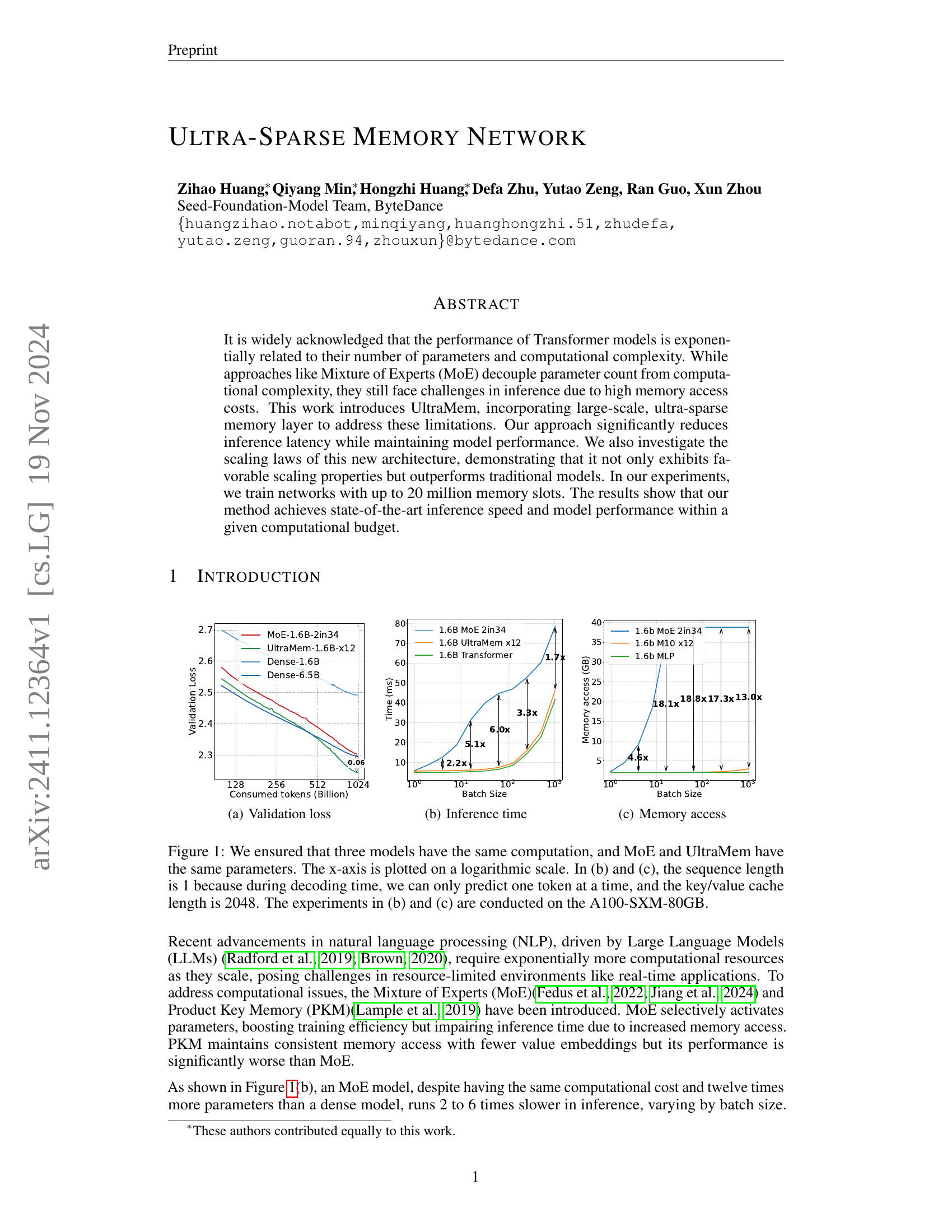
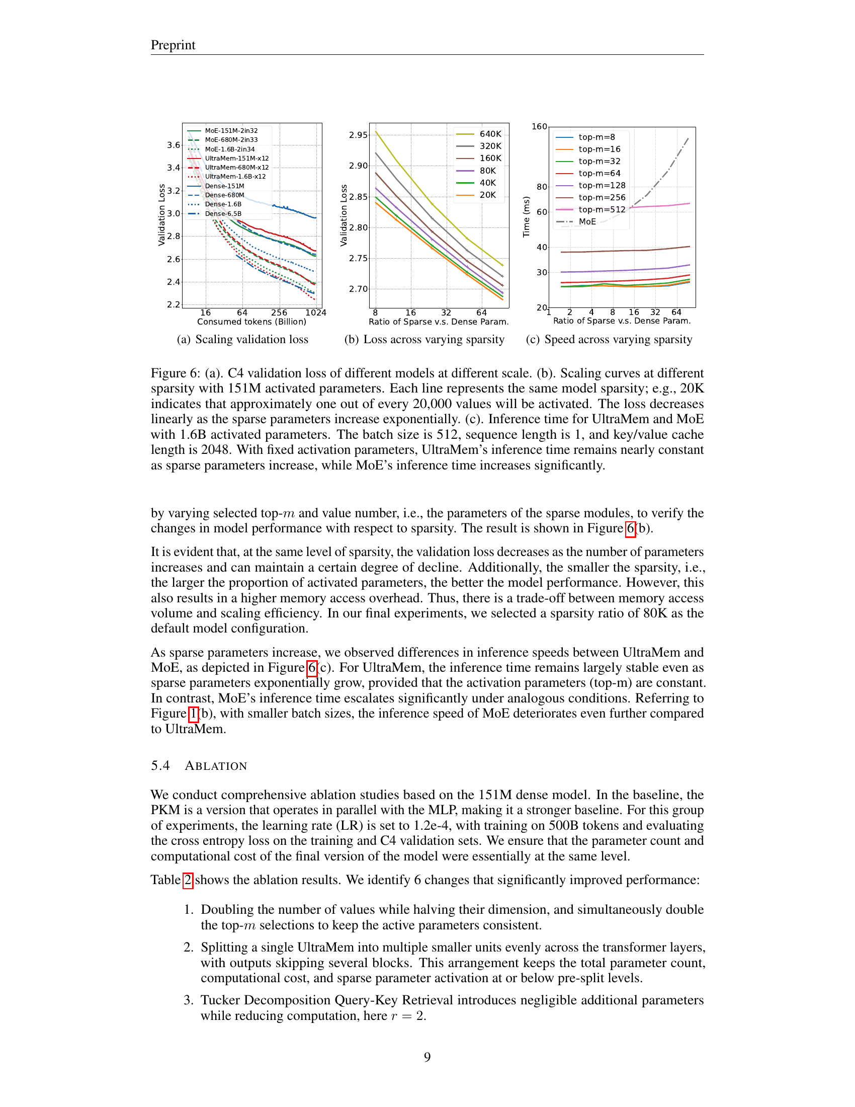
🔼 This figure shows the validation loss curves for various model architectures during training. The x-axis represents the number of consumed tokens (in billions) during training, indicating the training progress. The y-axis displays the validation loss, which is a measure of how well the model generalizes to unseen data. Lower validation loss signifies better generalization performance. Different lines represent different models, allowing for a comparison of their training performance and convergence rates. The models compared include dense models (with various numbers of parameters), MoE models (Mixture of Experts), and UltraMem models (the proposed model in this paper). The figure helps illustrate the effectiveness of UltraMem in maintaining performance while scaling up the model’s capacity.
read the caption
(a) Validation loss
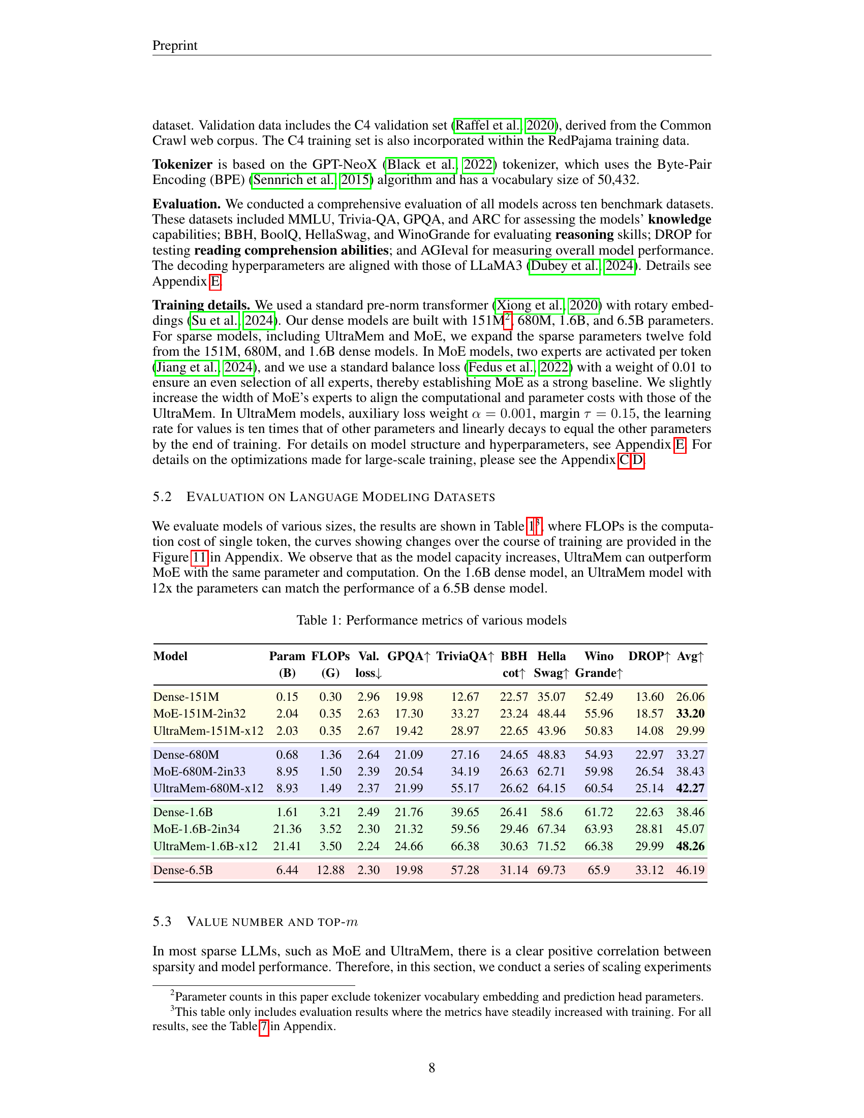
| Model | Param (B) | FLOPs (G) | Val. loss ↓ | GPQA ↑ | TriviaQA ↑ | BBH ↑ | HellaSwag ↑ | WinoGrande ↑ | Avg ↑ |
|---|---|---|---|---|---|---|---|---|---|
| Dense-151M | 0.15 | 0.30 | 2.96 | 19.98 | 12.67 | 22.57 | 35.07 | 52.49 | 26.06 |
| MoE-151M-2in32 | 2.04 | 0.35 | 2.63 | 17.30 | 33.27 | 23.24 | 48.44 | 55.96 | 33.20 |
| UltraMem-151M-x12 | 2.03 | 0.35 | 2.67 | 19.42 | 28.97 | 22.65 | 43.96 | 50.83 | 29.99 |
| Dense-680M | 0.68 | 1.36 | 2.64 | 21.09 | 27.16 | 24.65 | 48.83 | 54.93 | 33.27 |
| MoE-680M-2in33 | 8.95 | 1.50 | 2.39 | 20.54 | 34.19 | 26.63 | 62.71 | 59.98 | 38.43 |
| UltraMem-680M-x12 | 8.93 | 1.49 | 2.37 | 21.99 | 55.17 | 26.62 | 64.15 | 60.54 | 42.27 |
| Dense-1.6B | 1.61 | 3.21 | 2.49 | 21.76 | 39.65 | 26.41 | 58.6 | 61.72 | 38.46 |
| MoE-1.6B-2in34 | 21.36 | 3.52 | 2.30 | 21.32 | 59.56 | 29.46 | 67.34 | 63.93 | 45.07 |
| UltraMem-1.6B-x12 | 21.41 | 3.50 | 2.24 | 24.66 | 66.38 | 30.63 | 71.52 | 66.38 | 48.26 |
| Dense-6.5B | 6.44 | 12.88 | 2.30 | 19.98 | 57.28 | 31.14 | 69.73 | 65.9 | 46.19 |
🔼 This table presents a comparison of the performance metrics across different language models. It includes both dense models (standard Transformer architectures) and sparse models (Mixture of Experts (MoE) and Ultra-Sparse Memory Network (UltraMem)). The metrics shown are validation loss, and several downstream task performance scores (GPQA, TriviaQA, BBH, HellaSwag, Winogrande, DROP), along with the average score across these tasks. Model parameters and FLOPs (floating-point operations per second) are also provided to contextualize performance in relation to model size and computational cost.
read the caption
Table 1: Performance metrics of various models
In-depth insights#
UltraSparse Memory#
UltraSparse Memory Networks represent a novel approach to address the limitations of traditional Transformer models, particularly concerning their exponential scaling in parameters and computational complexity. By integrating a large-scale, ultra-sparse memory layer, UltraSparse Memory Networks significantly reduce inference latency without sacrificing model performance. This architecture achieves this by effectively decoupling parameter count from computational demands during inference. Unlike methods like Mixture of Experts (MoE), which face challenges due to high memory access costs, UltraSparse Memory Networks demonstrate favorable scaling properties, outperforming traditional models within a given computational budget. The ultra-sparse nature of the memory layer is a key innovation, enabling the handling of massive numbers of memory slots while maintaining efficient access. Further research will focus on fully exploring the scaling laws, exploring various sparsity configurations, and investigating the application of this architecture to larger language models. Ultimately, UltraSparse Memory Networks offer a promising path towards building larger, more efficient, and faster language models capable of handling more complex tasks.
Inference Speedup#
The concept of ‘Inference Speedup’ in the context of large language models (LLMs) centers on optimizing the efficiency of LLMs during the inference stage—the process of using a trained model to generate predictions on new input data. Traditional LLMs, due to their dense parameter structure, often exhibit slow inference speeds. The research explores methods to significantly enhance inference speeds, which is crucial for deploying LLMs in real-time applications. UltraMem, a novel architecture, addresses the challenges by utilizing large-scale, ultra-sparse memory layers, reducing memory access latency without sacrificing model performance. This sparse architecture contrasts with the dense parameter approach, resulting in a substantial inference speedup compared to Mixture of Experts (MoE) models and other existing methods. The study’s experimental validation shows that UltraMem achieves up to a 6x speedup over MoE while maintaining comparable performance. The scaling behavior is also analyzed, indicating that UltraMem’s speed advantage grows even more pronounced with larger batch sizes. This inference speedup, combined with UltraMem’s favorable scaling properties and state-of-the-art performance, makes it a compelling solution for various real-world applications demanding fast and accurate LLM inference.
Scaling Properties#
The scaling properties of large language models (LLMs) are a crucial area of research, focusing on how model performance changes with increased size and computational resources. Efficient scaling is paramount for cost-effectiveness and practicality. A key aspect involves understanding the relationship between the number of parameters, training data, and computational power, and how this impacts accuracy and inference speed. Mixture-of-Experts (MoE) models aim to decouple parameter count from computational cost, but face challenges in inference due to high memory access. The paper’s proposed UltraMem architecture attempts to address these limitations by incorporating a large-scale, ultra-sparse memory layer. This approach aims to achieve favorable scaling properties by significantly reducing inference latency while maintaining performance. The research delves into empirical demonstrations of UltraMem’s scaling laws, comparing its performance to traditional models and MoE, particularly with respect to the trade-offs between memory access and computation. The results aim to show UltraMem’s superior scaling behavior within a given computational budget, achieving state-of-the-art inference speed and model performance. The analysis likely investigates how UltraMem handles increased memory slots and addresses potential challenges in scaling its ultra-sparse memory layer.
Ablation Studies#
Ablation studies systematically remove components of a model to assess their individual contributions. In this context, the researchers likely conducted ablation experiments to understand the impact of various architectural choices and design decisions on the overall model performance. The goal is to isolate the effects of specific components and quantify their importance. For example, removing certain modules, like specific attention mechanisms or modifying the training process itself, and then measuring the performance drop enables researchers to understand which features are essential for performance. Results would reveal the relative importance of each component. Identifying critical elements helps refine model architecture, remove redundancy, and potentially guide future research focusing on improving the identified crucial parts of the model. Additionally, it helps to disentangle the complex interactions between different components and determine whether the contributions are additive or interactive. Overall, a comprehensive ablation study strengthens the paper by proving the effectiveness of the proposed methods and provides a better understanding of their underlying mechanisms.
Future Directions#
Future research could explore several promising avenues. Improving the efficiency of the key-value retrieval mechanism within UltraMem is crucial. Investigating alternative sparse attention mechanisms or exploring more advanced decomposition techniques beyond Tucker decomposition could significantly enhance performance and reduce computational costs. Extending UltraMem to other modalities beyond text, such as images or audio, presents a significant challenge but offers potential for broader applications. Investigating the scaling properties of UltraMem further is important to understand its limitations and opportunities at truly massive scales. This includes exploring different hardware architectures and training strategies to improve both training speed and inference efficiency. Finally, developing robust methods for handling expert imbalance in UltraMem is critical to ensuring its effectiveness across various downstream tasks and datasets. Thorough evaluation on diverse benchmark datasets is essential to validate its generalizability and compare it to state-of-the-art methods.
More visual insights#
More on figures

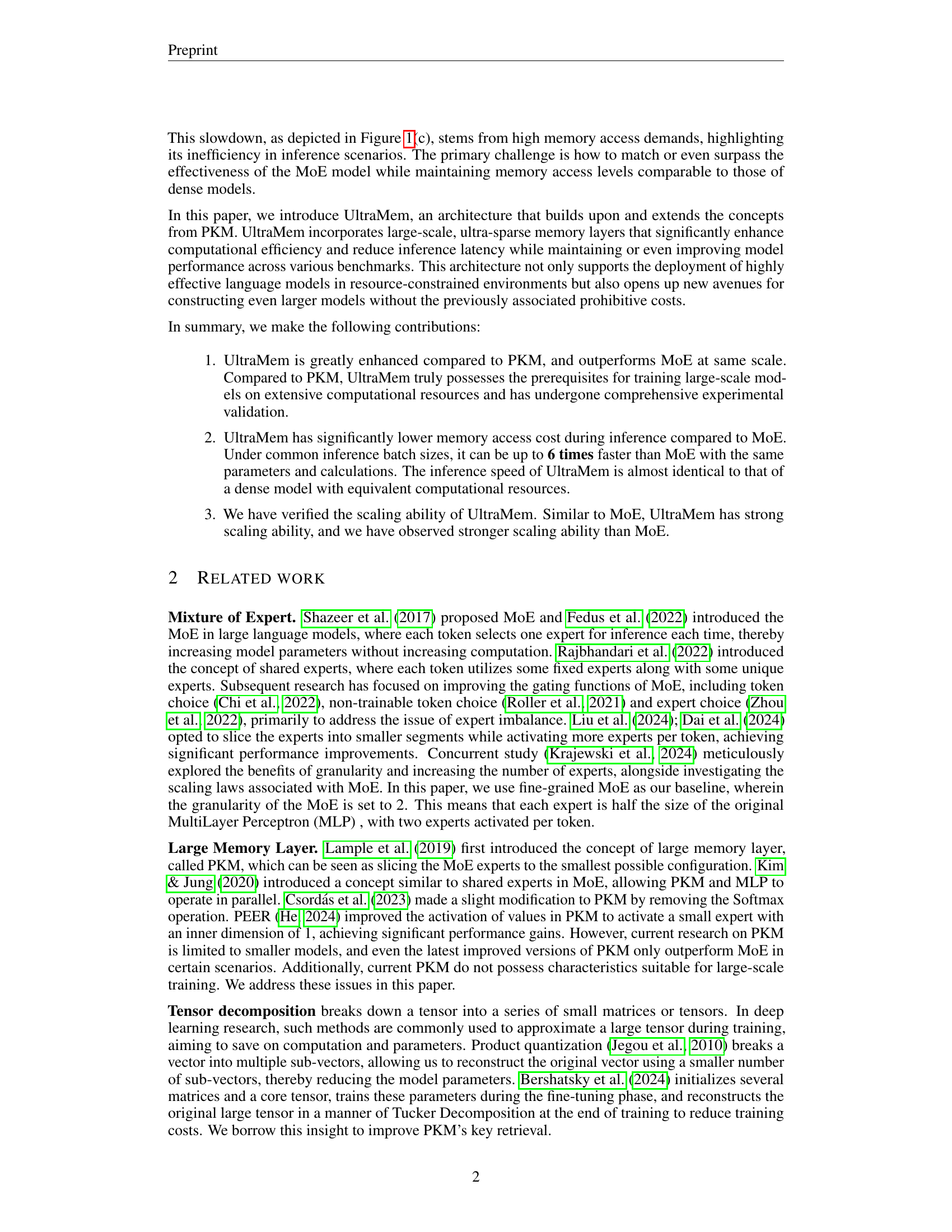
🔼 This figure shows the inference time of different Transformer models as the number of consumed tokens increases. The models compared are a dense Transformer, a Mixture-of-Experts (MoE) model, and the UltraMem model introduced in the paper. The x-axis represents the number of consumed tokens (in billions) and is plotted on a logarithmic scale. The y-axis represents the inference time in milliseconds. The figure demonstrates that UltraMem has significantly lower inference time than MoE, and comparable inference time with the dense Transformer, despite having the same computational cost and twelve times more parameters than the dense model.
read the caption
(b) Inference time

🔼 This figure displays the memory access (in GB) for different models across varying batch sizes. It shows how memory usage increases as batch size increases for different architectures. The models include a standard Transformer, Mixture of Experts (MoE), and the proposed UltraMem model. This visualization helps demonstrate the memory efficiency of UltraMem compared to traditional methods and MoE, particularly highlighting its lower memory footprint at larger batch sizes. The x-axis represents batch size (log scale), and the y-axis represents memory access (log scale).
read the caption
(c) Memory access

🔼 This figure compares the performance of three different model architectures: a standard Transformer, a Mixture-of-Experts (MoE) model, and the proposed Ultra-Sparse Memory Network (UltraMem). All three models were designed to have approximately the same computational cost, and the MoE and UltraMem models have the same number of parameters. The plots show how validation loss, inference time, and memory access vary as a function of the number of consumed tokens (a proxy for the input sequence length). The x-axis uses a logarithmic scale to better visualize the trends across different input sizes. For the inference time (b) and memory access (c) measurements, the sequence length was set to 1 (since only one token can be predicted at a time during inference), and the key/value cache length was set to 2048. The inference time and memory access tests were performed on an NVIDIA A100-SXM-80GB GPU.
read the caption
Figure 1: We ensured that three models have the same computation, and MoE and UltraMem have the same parameters. The x-axis is plotted on a logarithmic scale. In (b) and (c), the sequence length is 1 because during decoding time, we can only predict one token at a time, and the key/value cache length is 2048. The experiments in (b) and (c) are conducted on the A100-SXM-80GB.

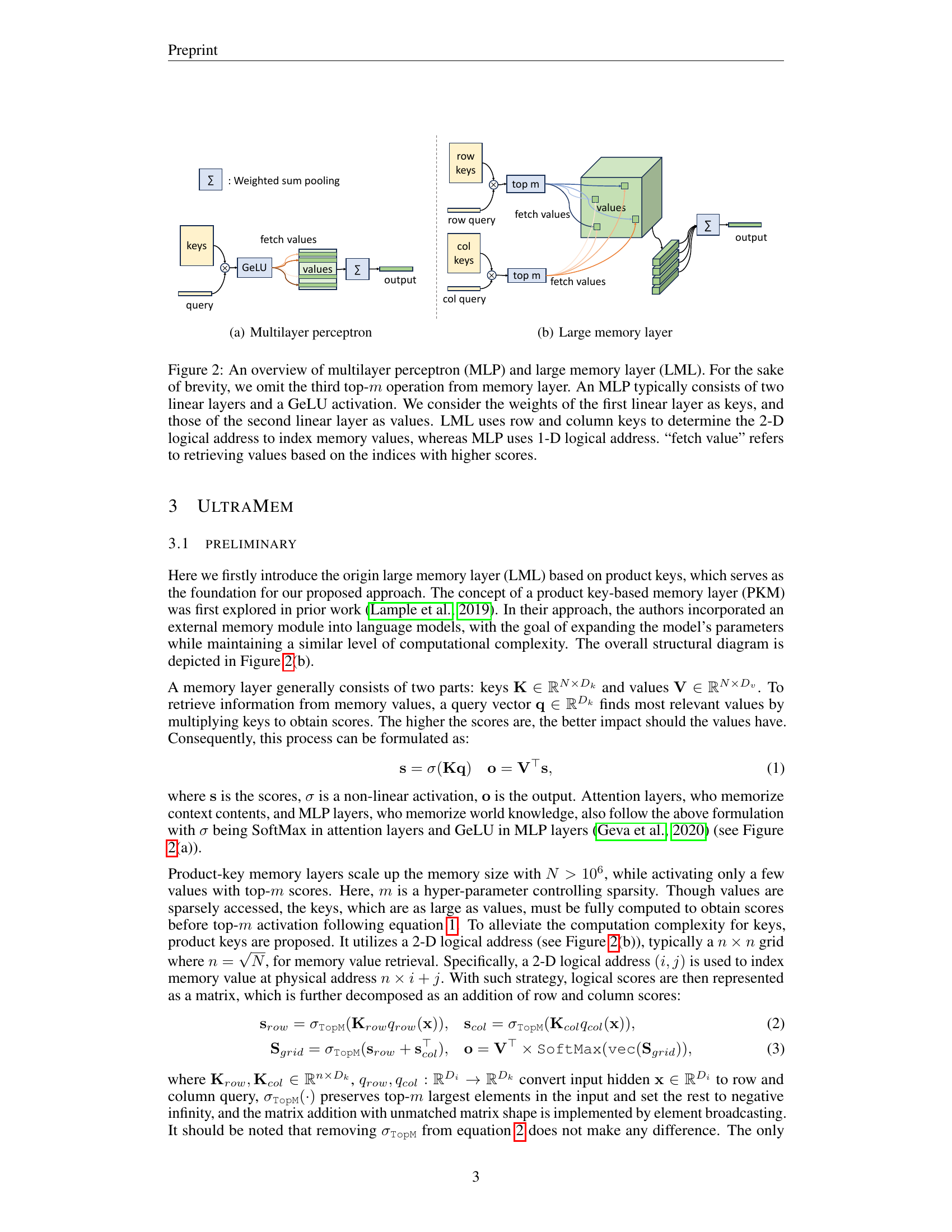
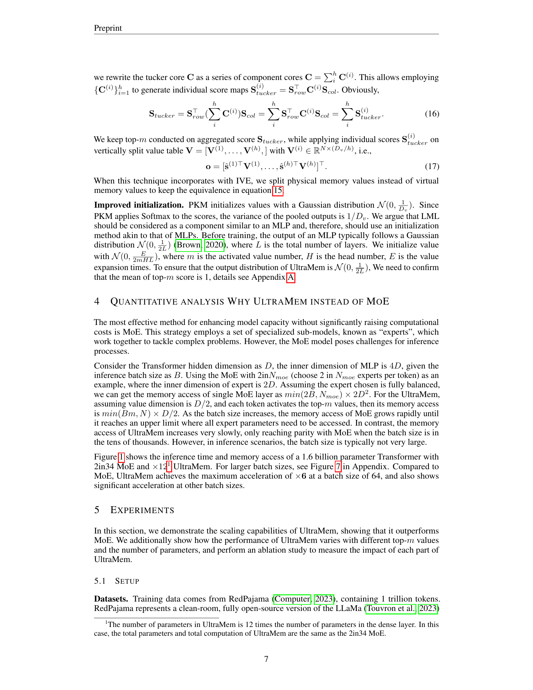
🔼 This figure shows the architecture of a Multilayer Perceptron (MLP), a fundamental component in many neural networks, including the UltraMem model discussed in the paper. An MLP consists of multiple layers of interconnected nodes (neurons), where each node performs a linear transformation followed by a non-linear activation function (GeLU in this case). The input to the network is transformed through multiple linear layers and activation functions. The final layer outputs the final result after multiple linear transformations and activation functions. The weights of the linear layers are represented as ‘keys’, and the outputs of the linear layers are referred to as ‘values’. This illustration emphasizes the role of these layers and their weights in the function of the MLP.
read the caption
(a) Multilayer perceptron

🔼 This figure shows the architecture of a large memory layer (LML) used in the UltraMem model. It illustrates how row and column keys are used to determine a 2D logical address to fetch values from a large-scale, ultra-sparse memory. This contrasts with a traditional MLP which utilizes a 1D logical address. The process of retrieving values based on indices with higher scores is also depicted.
read the caption
(b) Large memory layer

🔼 This figure provides a comparison of the architectures of a Multilayer Perceptron (MLP) and a Large Memory Layer (LML). The MLP, a standard component in neural networks, consists of two linear layers and a GeLU activation function. The weights of the first linear layer are interpreted as keys and the weights of the second linear layer as values. The LML, designed for efficient access to large memory, uses both row and column keys to create a 2-dimensional logical address, which allows for retrieving specific value vectors from a memory space. This contrasts with the MLP, which uses a simpler 1-dimensional logical address for accessing values. The process of selecting the most relevant values based on their indices and associated scores is denoted as ‘fetch value’. The third top-m operation in the LML, a step to select only the most relevant m values, is omitted for brevity in this diagram.
read the caption
Figure 2: An overview of multilayer perceptron (MLP) and large memory layer (LML). For the sake of brevity, we omit the third top-m𝑚mitalic_m operation from memory layer. An MLP typically consists of two linear layers and a GeLU activation. We consider the weights of the first linear layer as keys, and those of the second linear layer as values. LML uses row and column keys to determine the 2-D logical address to index memory values, whereas MLP uses 1-D logical address. “fetch value” refers to retrieving values based on the indices with higher scores.

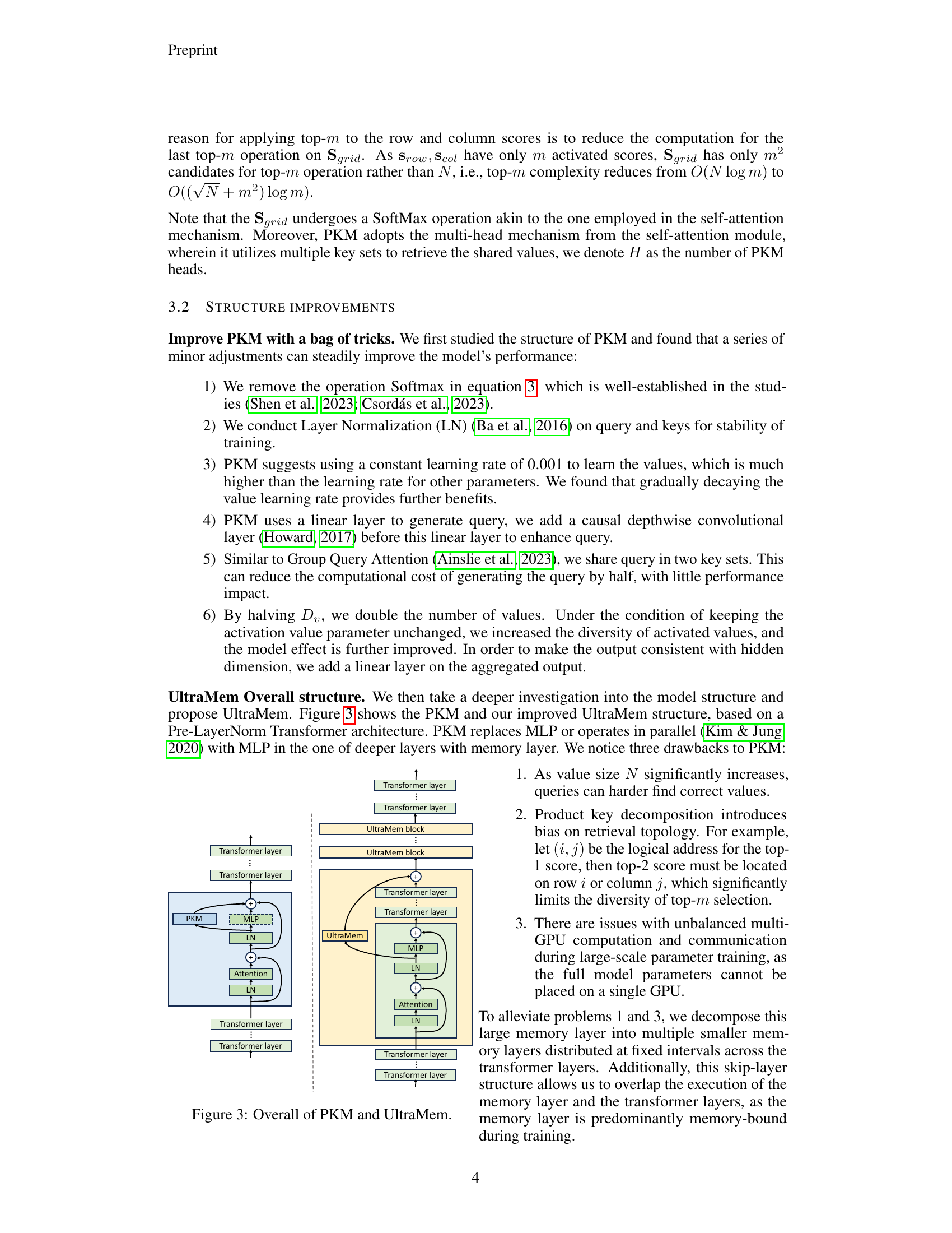
🔼 This figure provides a visual comparison of the Product-Key Memory (PKM) architecture and the proposed UltraMem architecture. PKM is shown to integrate a memory layer in parallel or in place of an MLP layer within a standard Transformer architecture. UltraMem improves upon PKM by decomposing the large memory layer into multiple smaller layers distributed across multiple Transformer layers. This allows for greater efficiency and scalability by overlapping the execution of memory and Transformer layers.
read the caption
Figure 3: Overall of PKM and UltraMem.

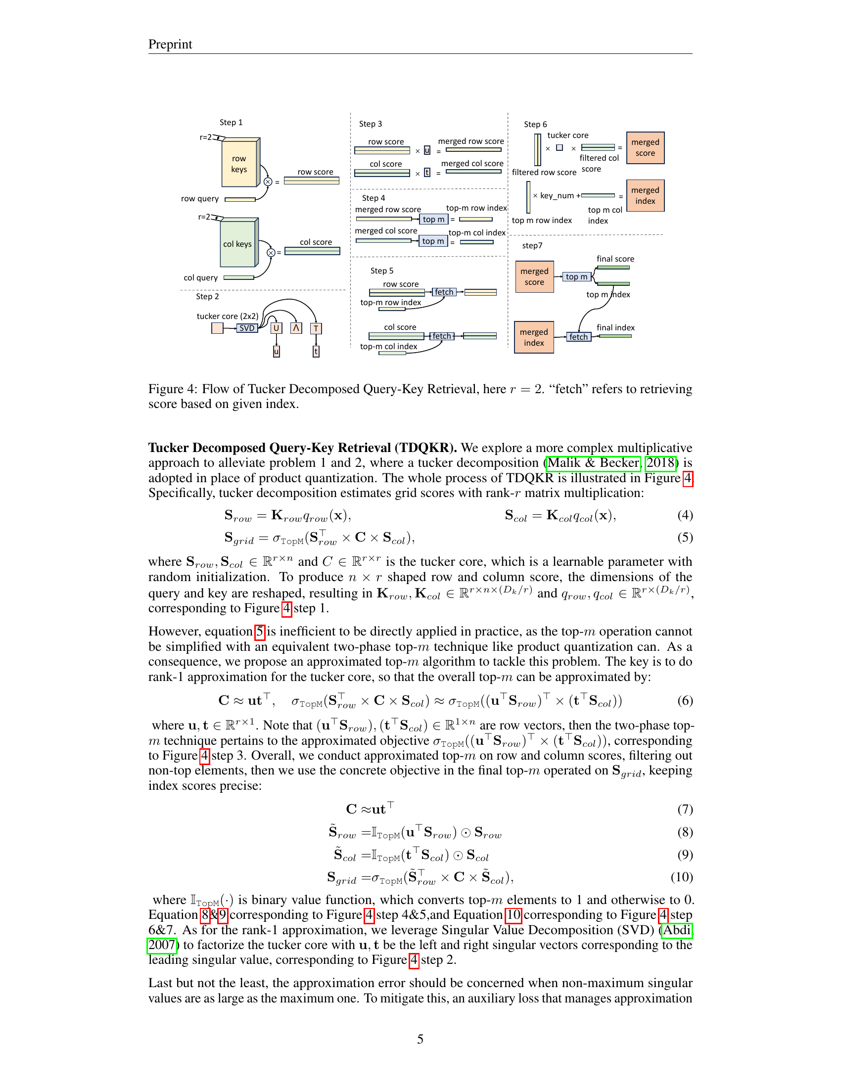
🔼 This figure illustrates the Tucker Decomposed Query-Key Retrieval (TDQKR) method, a technique used to improve the efficiency of retrieving relevant values from a large memory layer. The process begins with a query (x) which is transformed into row and column queries through two linear projections. These queries are then used to calculate row scores and column scores based on product keys (Krow and Kcol). A Tucker decomposition of rank-r (in this case r=2) is applied to these scores to form a score grid (Sgrid). The Tucker decomposition uses a core tensor (C) which significantly reduces the computational cost compared to a full matrix multiplication. Finally, the top-m largest values from Sgrid are selected, their indices are determined, and the corresponding values from the memory are retrieved. The diagram visually represents the step-by-step flow of the process, highlighting the key steps and operations involved in the TDQKR method.
read the caption
Figure 4: Flow of Tucker Decomposed Query-Key Retrieval, here r=2𝑟2r=2italic_r = 2. “fetch” refers to retrieving score based on given index.

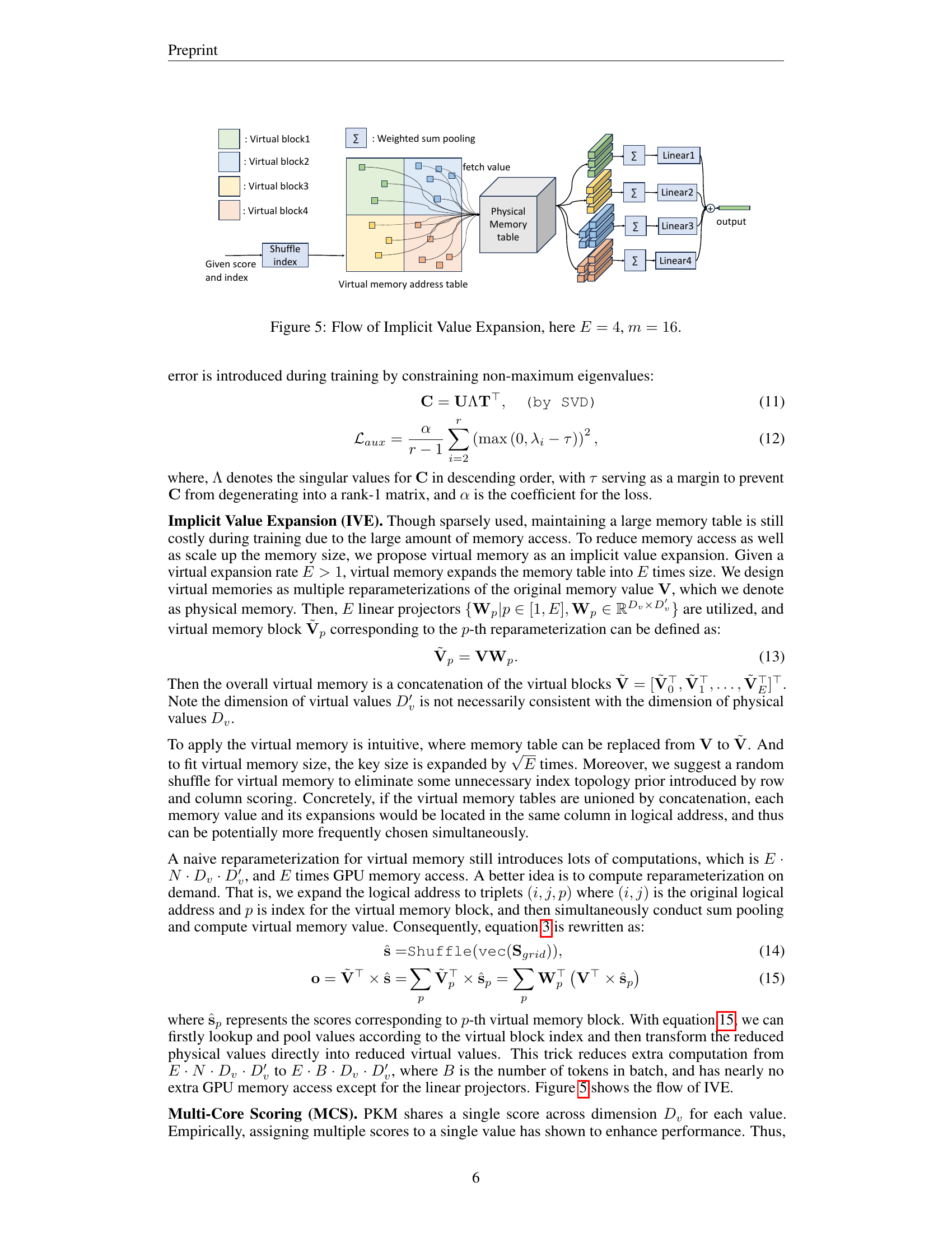
🔼 This figure illustrates the process of Implicit Value Expansion (IVE) in UltraMem, a technique to reduce memory access during training. The figure shows how, with an expansion rate of E=4, the original memory values (V) are expanded into four virtual memory blocks (V1, V2, V3, V4). Each virtual block is a reparameterized version of the original value, created using linear projectors (Wp). This expansion increases the effective size of the memory table without proportionally increasing memory access costs. A shuffle operation is applied to the virtual memory addresses to further enhance memory access efficiency. The figure also demonstrates how the virtual blocks are accessed using linear layers (Linear1-4) and weighted sum pooling (Σ) to produce the final output. The ’m’ parameter refers to the sparsity, here it is 16, meaning only top 16 values are considered for the next step.
read the caption
Figure 5: Flow of Implicit Value Expansion, here E=4𝐸4E=4italic_E = 4, m=16𝑚16m=16italic_m = 16.

🔼 This figure shows the C4 validation loss for different models across various scales. The x-axis represents the number of consumed tokens (in billions) during training, while the y-axis represents the validation loss. Different lines represent different models, including dense models (Dense-151M, Dense-680M, Dense-1.6B, Dense-6.5B) and sparse models (UltraMem-151M-x12, UltraMem-680M-x12, UltraMem-1.6B-x12, MoE-151M-2in32, MoE-680M-2in33, MoE-1.6B-2in34). The plot demonstrates how the validation loss decreases as the number of consumed tokens increases for all models, with the dense models generally exhibiting lower loss than the sparse models. The figure illustrates the scaling behavior of different model architectures in terms of training loss.
read the caption
(a) Scaling validation loss

🔼 This figure shows the validation loss of different models with varying sparsity levels while maintaining the same number of activated parameters. Each line represents a different sparsity level; for example, 20K indicates approximately 1 in 20,000 values are activated. The x-axis represents the ratio of sparse to dense parameters, showcasing how the model’s capacity scales with different sparsity levels. The y-axis shows the validation loss. This graph demonstrates the relationship between model sparsity and performance during training.
read the caption
(b) Loss across varying sparsity

🔼 This figure shows the inference speed of UltraMem and MoE models with 1.6 billion activated parameters. The x-axis represents the ratio of sparse parameters to dense parameters, illustrating different sparsity levels. The y-axis shows the inference time in milliseconds. The plot demonstrates that UltraMem’s inference speed remains relatively constant even as sparsity increases, unlike MoE, whose inference time increases significantly with increasing sparsity. This highlights UltraMem’s efficiency and robustness in inference scenarios.
read the caption
(c) Speed across varying sparsity

🔼 Figure 6 presents a comparison of UltraMem and MoE model performance across different scales and sparsity levels. Subfigure (a) shows the validation loss on the C4 dataset for various model sizes, demonstrating the scaling behavior. Subfigure (b) focuses on the impact of sparsity, showing that while UltraMem’s loss decreases linearly with exponentially increasing parameters, MoE’s performance is significantly affected by sparsity. Subfigure (c) compares the inference time of UltraMem and MoE with 1.6B activated parameters under different sparsity levels, highlighting that UltraMem exhibits significantly better inference speed at larger sparsity.
read the caption
Figure 6: (a). C4 validation loss of different models at different scale. (b). Scaling curves at different sparsity with 151M activated parameters. Each line represents the same model sparsity; e.g., 20K indicates that approximately one out of every 20,000 values will be activated. The loss decreases linearly as the sparse parameters increase exponentially. (c). Inference time for UltraMem and MoE with 1.6B activated parameters. The batch size is 512, sequence length is 1, and key/value cache length is 2048. With fixed activation parameters, UltraMem’s inference time remains nearly constant as sparse parameters increase, while MoE’s inference time increases significantly.

🔼 This figure shows the inference time of different models with varying batch sizes. The x-axis represents the batch size, and the y-axis represents the inference time in milliseconds. The models compared include a dense Transformer, MoE (Mixture of Experts), and UltraMem. The figure illustrates that UltraMem achieves significantly faster inference times compared to MoE, particularly at smaller batch sizes, while maintaining performance comparable to the dense model.
read the caption
(a) Inference time

🔼 The figure shows the memory access in gigabytes (GB) of three different model architectures: a dense Transformer model, a Mixture of Experts (MoE) model, and an Ultra-Sparse Memory Network (UltraMem) model. The x-axis represents the batch size, showing how memory usage scales with increasing batch size. The plot demonstrates that UltraMem has significantly lower memory access compared to MoE, especially at smaller batch sizes, while remaining comparable to a dense model.
read the caption
(b) Memory access

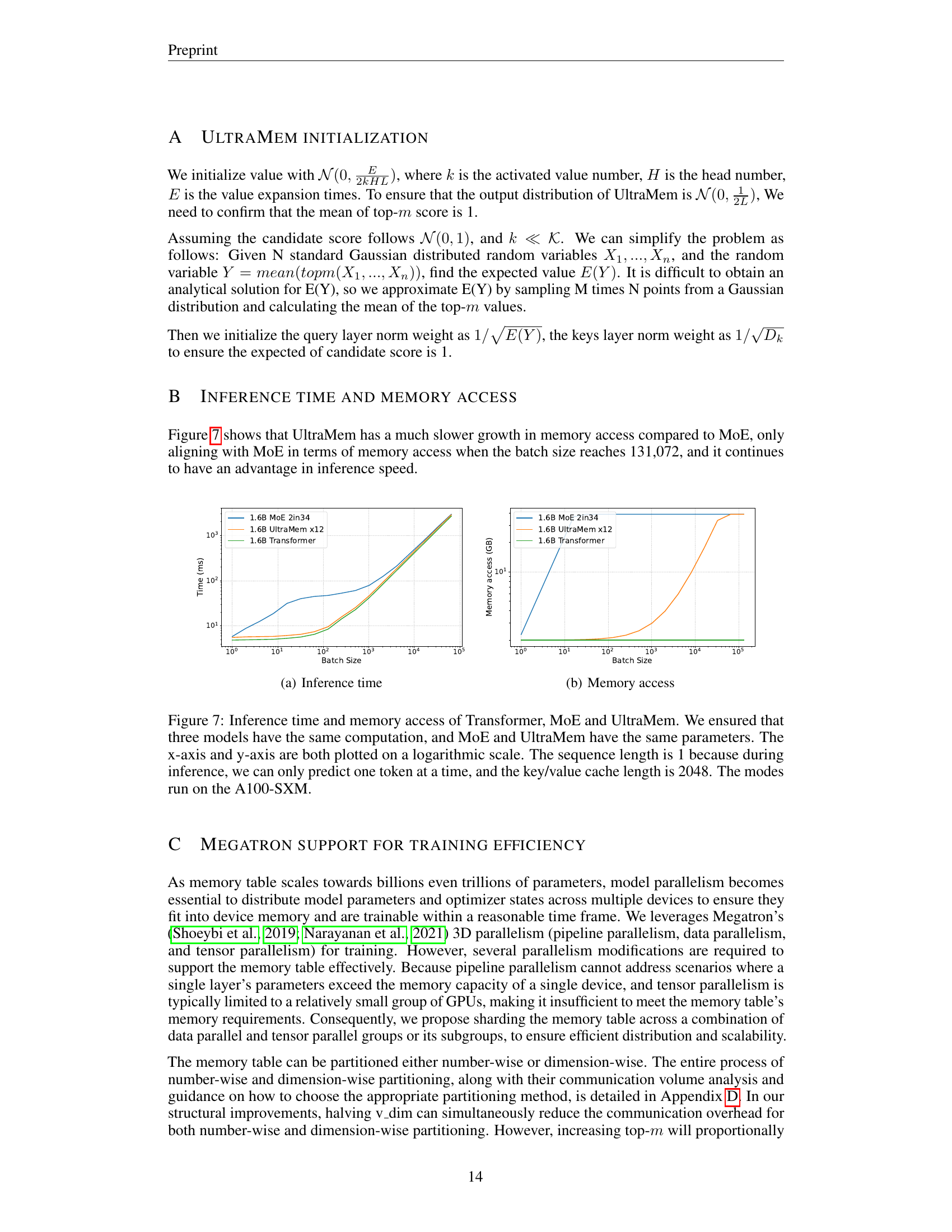
🔼 This figure compares the inference time and memory access of three different model architectures: a standard Transformer, a Mixture of Experts (MoE) model, and the proposed Ultra-Sparse Memory Network (UltraMem). All three models were designed to have the same computational complexity and number of parameters. The x-axis shows the batch size (on a logarithmic scale), and the y-axis shows either inference time or memory access (also on a logarithmic scale). The sequence length is fixed at 1 because, during inference, only one token can be predicted at a time. The key/value cache length is set to 2048. The experiments were conducted on an A100-SXM GPU. The graph visually demonstrates UltraMem’s superior performance in terms of both inference speed and memory efficiency, especially as batch size increases.
read the caption
Figure 7: Inference time and memory access of Transformer, MoE and UltraMem. We ensured that three models have the same computation, and MoE and UltraMem have the same parameters. The x-axis and y-axis are both plotted on a logarithmic scale. The sequence length is 1 because during inference, we can only predict one token at a time, and the key/value cache length is 2048. The modes run on the A100-SXM.

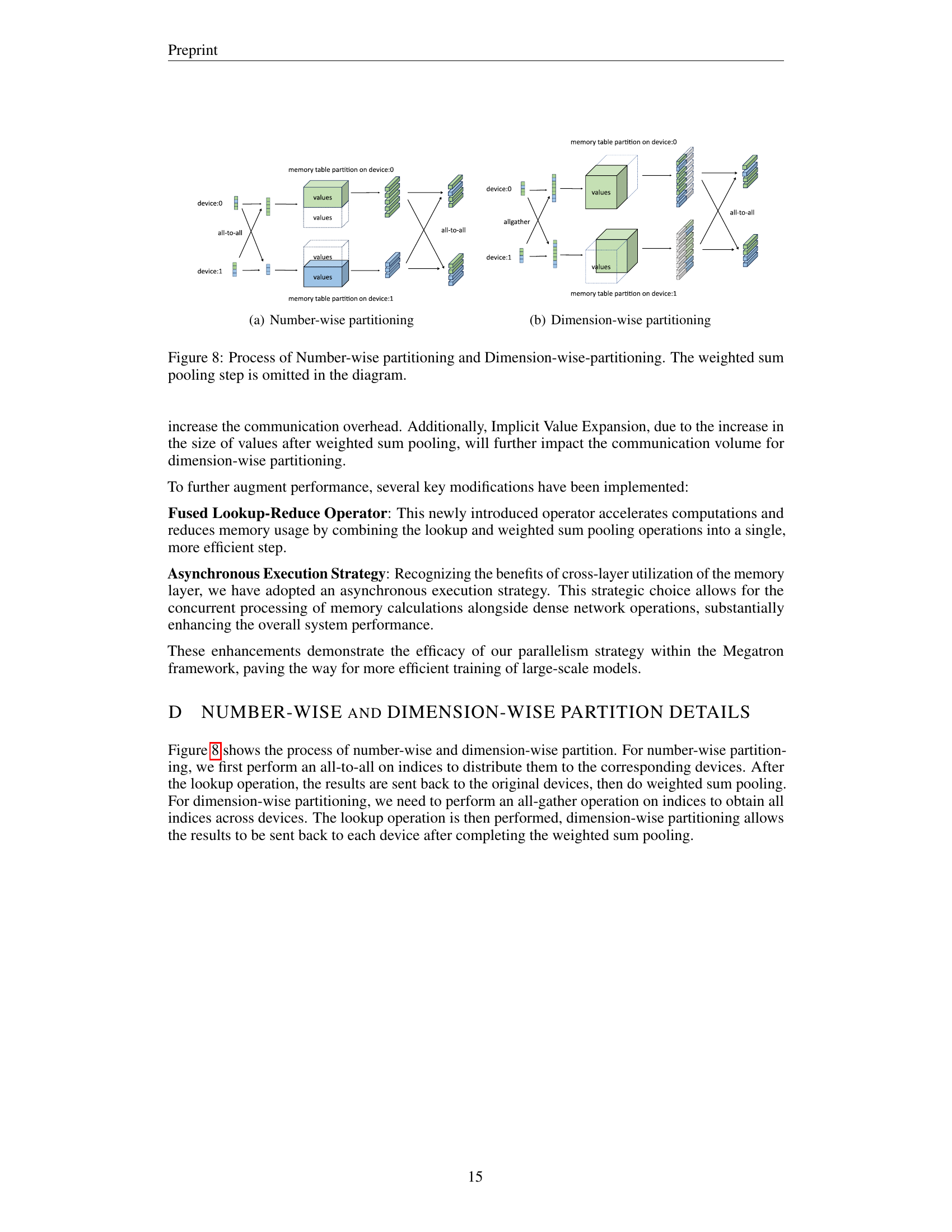
🔼 This figure illustrates the number-wise partitioning strategy used in the UltraMem model for efficient parallel processing of large memory tables. In number-wise partitioning, the memory table is divided into multiple parts, each assigned to a different device or GPU. The indices are initially distributed across all devices using an all-to-all communication operation. After the lookup operation retrieves the necessary values from the memory table partitions, the results are sent back to the original devices for the weighted sum pooling operation. This method optimizes memory access and communication efficiency during training by distributing the workload.
read the caption
(a) Number-wise partitioning

🔼 This figure illustrates the process of dimension-wise partitioning of the memory table across multiple devices in a parallel training setup. The memory table is initially partitioned across devices. An all-gather operation is performed on indices, meaning each device obtains all indices from all devices. Subsequently, a lookup operation is carried out on all devices using the gathered indices, which retrieves the values from the corresponding partitions of the memory table. Finally, a dimension-wise reduction is performed, generating a final aggregated result that combines contributions from all the devices. This approach effectively leverages distributed computation to handle large memory tables in parallel training.
read the caption
(b) Dimension-wise partitioning

🔼 This figure illustrates the data parallelism strategies used for the memory table in UltraMem, specifically focusing on the number-wise and dimension-wise partitioning methods. Number-wise partitioning involves dividing the memory table among multiple devices, where each device handles a portion of the values. An all-to-all communication step is shown to distribute indices across devices, followed by individual devices performing lookups and sending the results back. Dimension-wise partitioning instead distributes the dimensions of the memory table across devices, requiring an all-gather step to collect all indices. Lookups are then performed, and the results are aggregated and sent back to each device. The weighted sum pooling operation, which is a crucial part of the memory table processing, is omitted for simplicity.
read the caption
Figure 8: Process of Number-wise partitioning and Dimension-wise-partitioning. The weighted sum pooling step is omitted in the diagram.

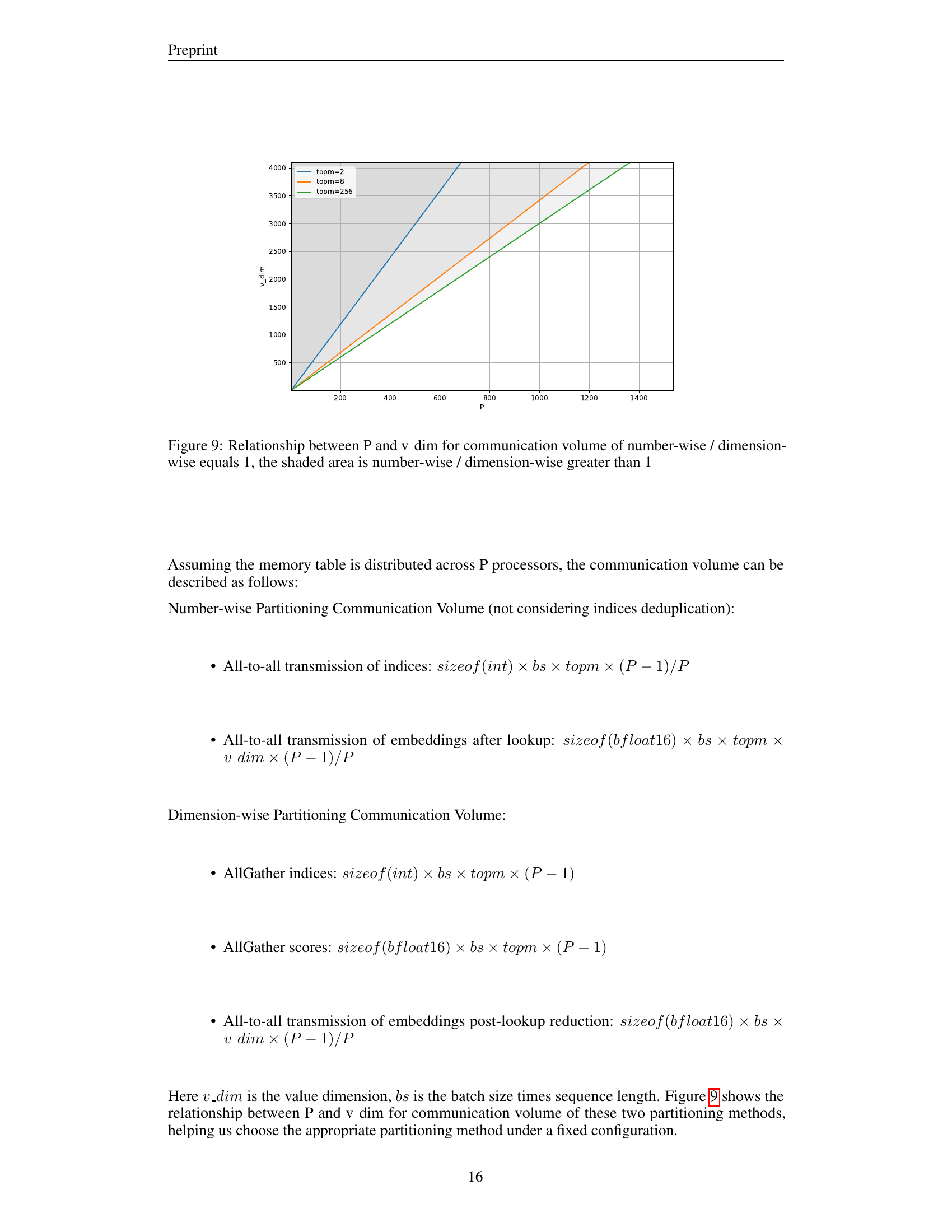
🔼 Figure 9 illustrates the trade-off between the number of processors (P) and the value dimension (v_dim) when choosing between number-wise and dimension-wise partitioning strategies for the memory table in UltraMem. The communication volume is compared for both methods, showing that number-wise partitioning is preferable in the unshaded area (number-wise volume < dimension-wise volume), while dimension-wise partitioning becomes advantageous in the shaded region. Different top-m values impact this tradeoff, altering the regions of preference for each partitioning strategy. This figure helps guide the selection of the optimal partitioning strategy based on the system configuration (number of processors and value dimension).
read the caption
Figure 9: Relationship between P and v_dim for communication volume of number-wise / dimension-wise equals 1, the shaded area is number-wise / dimension-wise greater than 1

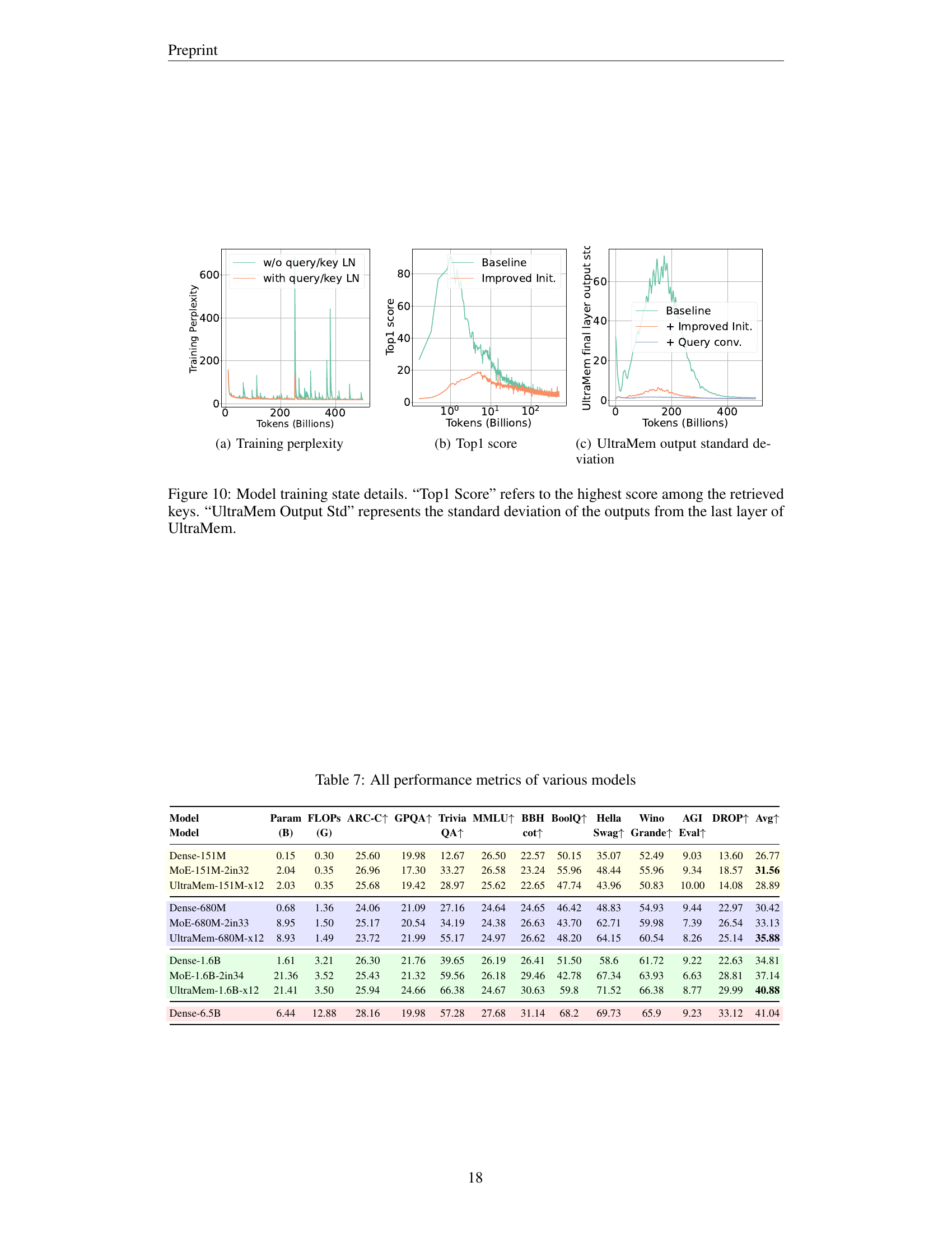
🔼 This figure displays the training perplexity of different models over the course of training. The x-axis represents the number of tokens processed during training (in billions), while the y-axis shows the training perplexity. Different lines represent different models, allowing for a comparison of their training performance. Lower perplexity indicates better model performance. The plot shows the learning curves, demonstrating how the perplexity decreases (ideally) over time as the model learns from the data.
read the caption
(a) Training perplexity

🔼 The graph displays the top-1 score achieved during the training process of the UltraMem model. The top-1 score represents the highest score among all retrieved keys in the memory layer, indicating the relevance of the retrieved values. The x-axis denotes the number of tokens processed during training, while the y-axis shows the top-1 score. The plot illustrates how the top-1 score evolves throughout training, providing insights into the model’s ability to retrieve relevant information from its memory.
read the caption
(b) Top1 score

🔼 This figure shows the standard deviation of the outputs from the last layer of the UltraMem model during training. It helps to visualize the stability and consistency of the model’s predictions over time and across different parts of the training data. Lower standard deviation indicates more stable and consistent predictions.
read the caption
(c) UltraMem output standard deviation
More on tables
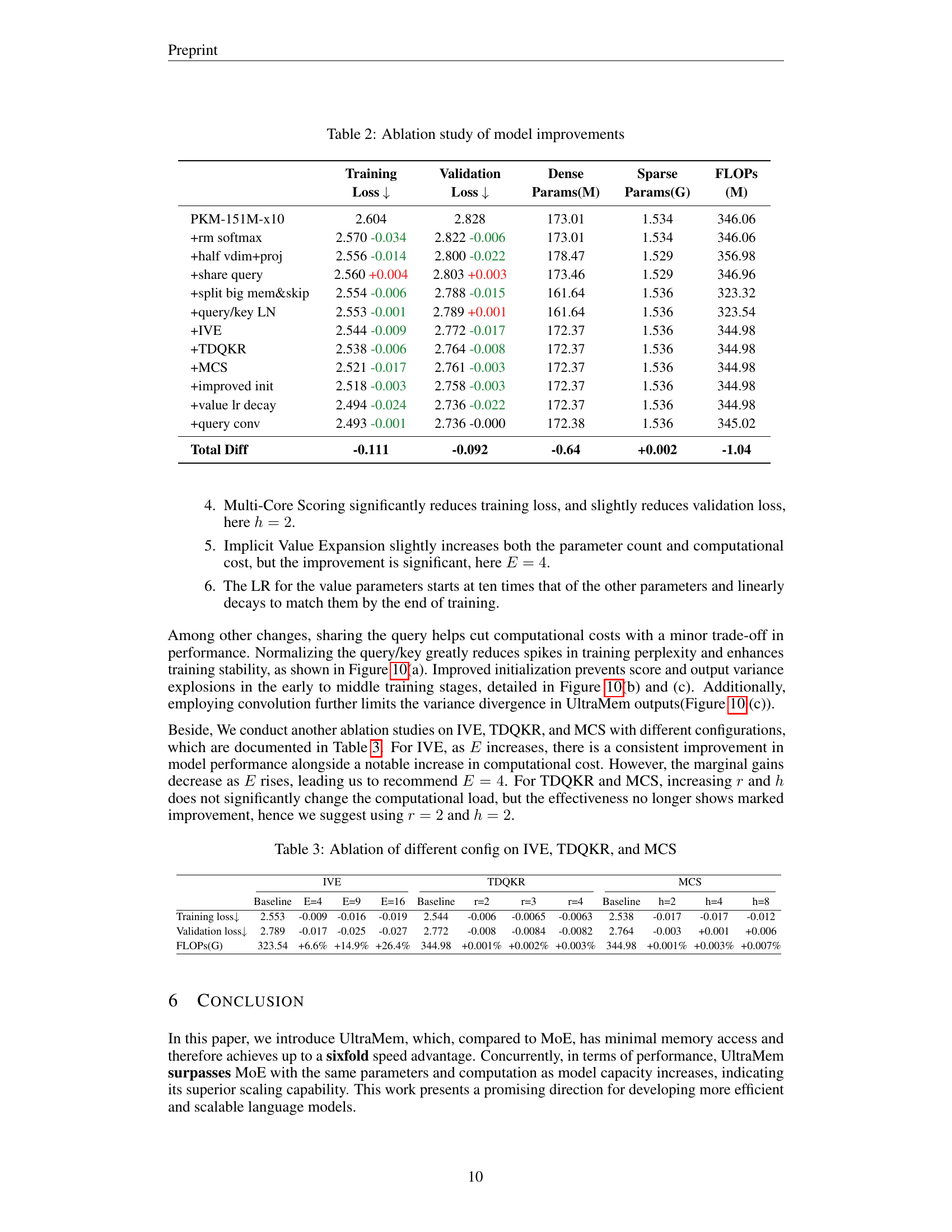
| Model | Training Loss ↓ | Validation Loss ↓ | Dense Params (M) | Sparse Params (G) | FLOPs (M) |
|---|---|---|---|---|---|
| PKM-151M-x10 | 2.604 | 2.828 | 173.01 | 1.534 | 346.06 |
| +rm softmax | 2.570 (-0.034) | 2.822 (-0.006) | 173.01 | 1.534 | 346.06 |
| +half vdim+proj | 2.556 (-0.014) | 2.800 (-0.022) | 178.47 | 1.529 | 356.98 |
| +share query | 2.560 (+0.004) | 2.803 (+0.003) | 173.46 | 1.529 | 346.96 |
| +split big mem&skip | 2.554 (-0.006) | 2.788 (-0.015) | 161.64 | 1.536 | 323.32 |
| +query/key LN | 2.553 (-0.001) | 2.789 (+0.001) | 161.64 | 1.536 | 323.54 |
| +IVE | 2.544 (-0.009) | 2.772 (-0.017) | 172.37 | 1.536 | 344.98 |
| +TDQKR | 2.538 (-0.006) | 2.764 (-0.008) | 172.37 | 1.536 | 344.98 |
| +MCS | 2.521 (-0.017) | 2.761 (-0.003) | 172.37 | 1.536 | 344.98 |
| +improved init | 2.518 (-0.003) | 2.758 (-0.003) | 172.37 | 1.536 | 344.98 |
| +value lr decay | 2.494 (-0.024) | 2.736 (-0.022) | 172.37 | 1.536 | 344.98 |
| +query conv | 2.493 (-0.001) | 2.736 (0.000) | 172.38 | 1.536 | 345.02 |
| Total Diff | -0.111 | -0.092 | -0.64 | +0.002 | -1.04 |
🔼 This table presents the results of an ablation study that systematically evaluates the impact of various design choices on the performance of the UltraMem model. Each row represents a variation of the model, differing in a single aspect from the previous row. The table shows the training and validation loss, the number of dense and sparse parameters, and the FLOPS (floating point operations per second). By comparing the performance metrics across rows, the study quantifies the contribution of each modification to the overall model’s effectiveness.
read the caption
Table 2: Ablation study of model improvements
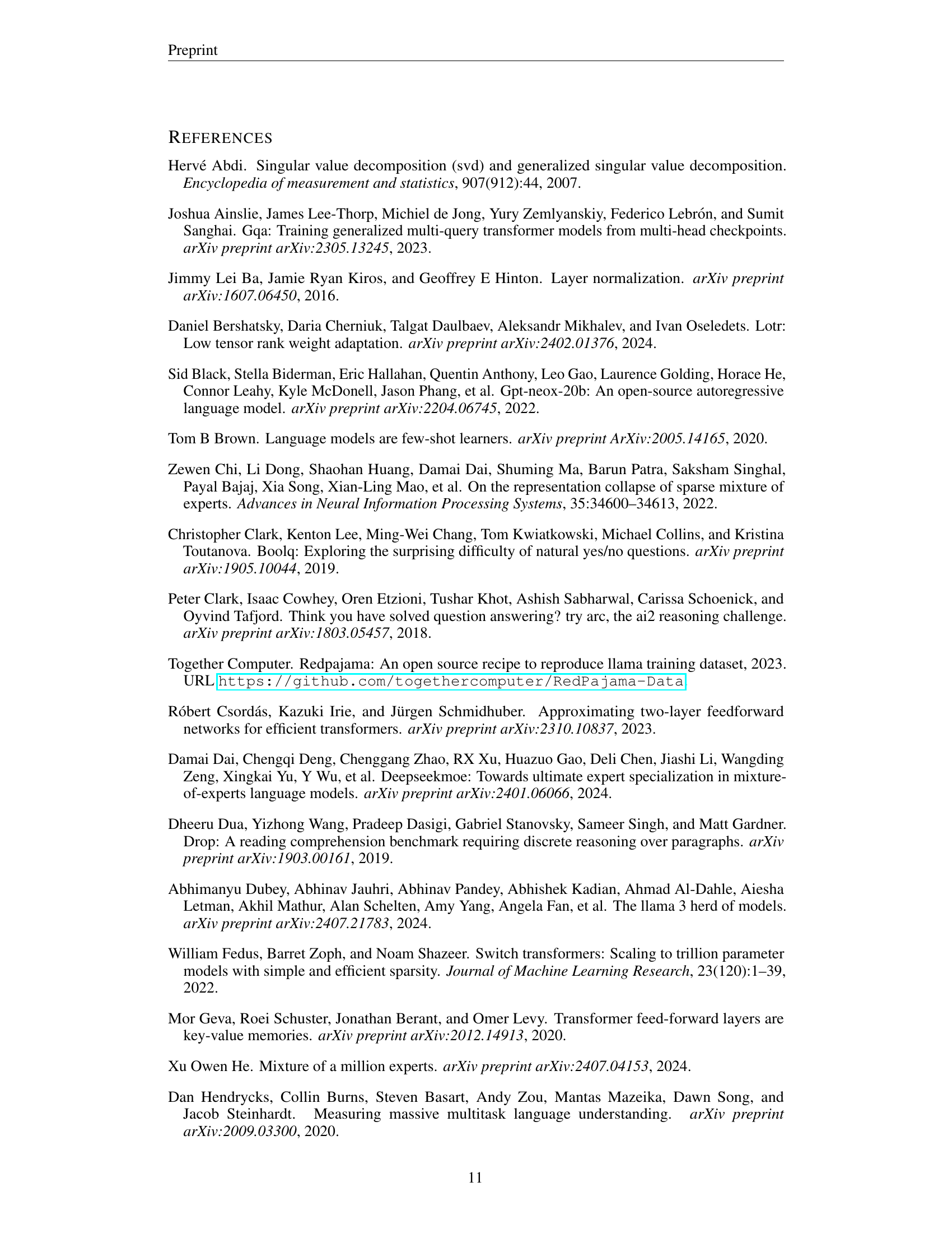
| IVE | TDQKR | MCS | |||||||||||
|---|---|---|---|---|---|---|---|---|---|---|---|---|---|
| Baseline | E=4 | E=9 | E=16 | Baseline | r=2 | r=3 | r=4 | Baseline | h=2 | h=4 | h=8 | ||
| Training loss ↓ | 2.553 | -0.009 | -0.016 | -0.019 | 2.544 | -0.006 | -0.0065 | -0.0063 | 2.538 | -0.017 | -0.017 | -0.012 | |
| Validation loss ↓ | 2.789 | -0.017 | -0.025 | -0.027 | 2.772 | -0.008 | -0.0084 | -0.0082 | 2.764 | -0.003 | +0.001 | +0.006 | |
| FLOPs(G) | 323.54 | +6.6% | +14.9% | +26.4% | 344.98 | +0.001% | +0.002% | +0.003% | 344.98 | +0.001% | +0.003% | +0.007% |
🔼 This table presents the results of ablation studies conducted to evaluate the impact of different configurations on the performance of the UltraMem model. Specifically, it analyzes the effects of Implicit Value Expansion (IVE), Tucker Decomposed Query-Key Retrieval (TDQKR), and Multi-Core Scoring (MCS) on both training loss and validation loss. Different hyperparameters are tested for each component, allowing for a detailed comparison of their individual contributions to the overall model performance. The table shows the training and validation losses, number of parameters, and FLOPS for various configurations, enabling a quantitative assessment of the effectiveness of each ablation.
read the caption
Table 3: Ablation of different config on IVE, TDQKR, and MCS
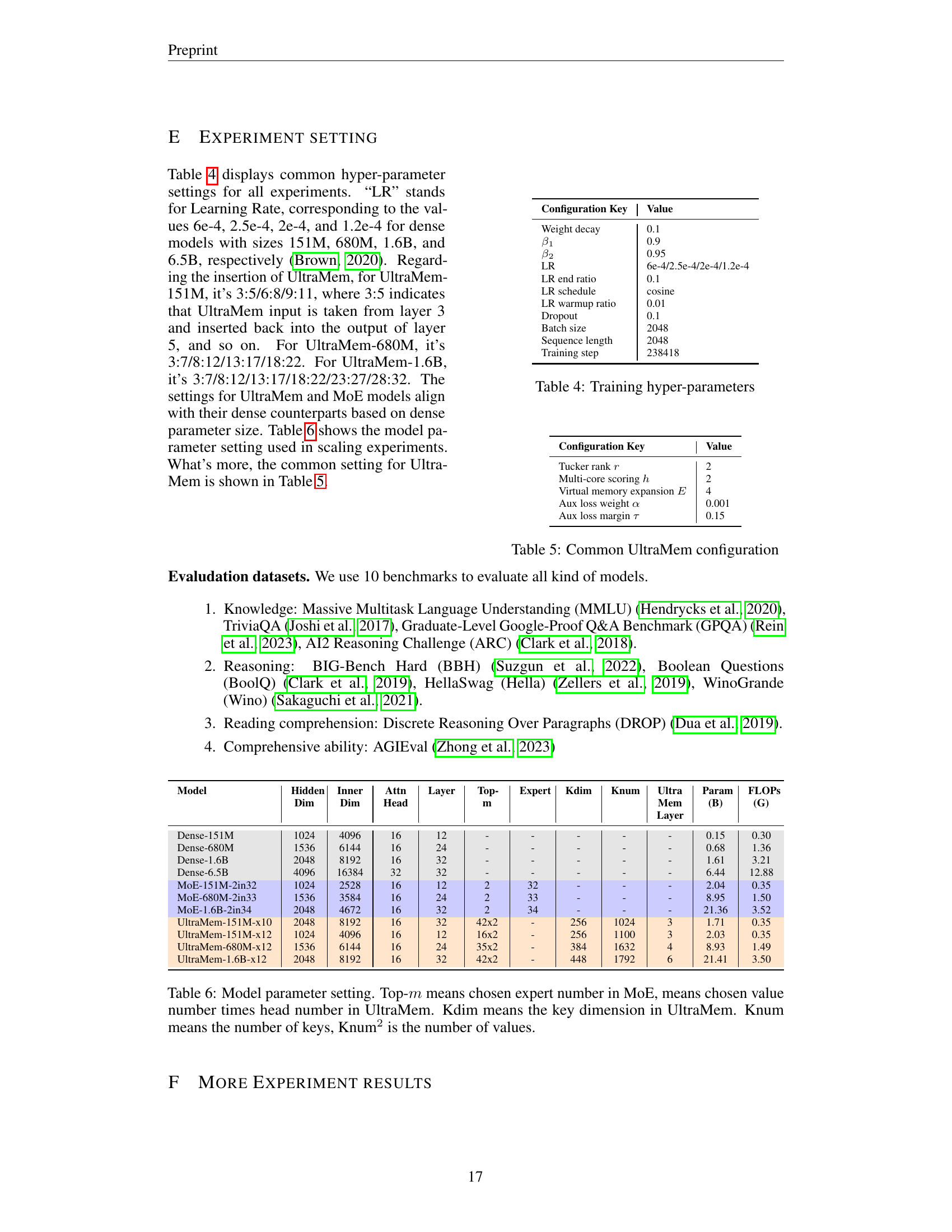
| Configuration Key | Value |
|---|---|
| Weight decay | 0.1 |
| β₁ | 0.9 |
| β₂ | 0.95 |
| LR | 6e-4/2.5e-4/2e-4/1.2e-4 |
| LR end ratio | 0.1 |
| LR schedule | cosine |
| LR warmup ratio | 0.01 |
| Dropout | 0.1 |
| Batch size | 2048 |
| Sequence length | 2048 |
| Training step | 238418 |
🔼 This table lists the hyperparameters used during the training phase of the models in the paper. It details settings for various aspects of the training process, including weight decay, optimization parameters (β1 and β2 for Adam), learning rate (LR) and its scheduling, dropout rate, batch size, sequence length, and the total number of training steps. Learning rates are specified for models with varying parameter counts (151M, 680M, 1.6B, and 6.5B parameters).
read the caption
Table 4: Training hyper-parameters
| Configuration Key | Value |
|---|---|
| Tucker rank r | 2 |
| Multi-core scoring h | 2 |
| Virtual memory expansion E | 4 |
| Aux loss weight α | 0.001 |
| Aux loss margin τ | 0.15 |
🔼 This table details the common hyperparameters used in configuring the UltraMem model. It lists key settings and their corresponding values, providing essential information for understanding and replicating the experimental setup. These values were used consistently across the experiments involving the UltraMem model, ensuring consistency and comparability of results.
read the caption
Table 5: Common UltraMem configuration
| Model | Param | FLOPs | ARC-C↑ | GPQA↑ | Trivia | MMLU↑ | BBH | BoolQ↑ | Hella | Wino | AGI | DROP↑ | Avg↑ | |
|---|---|---|---|---|---|---|---|---|---|---|---|---|---|---|
| Dense-151M | 0.15 | 0.30 | 25.60 | 19.98 | 12.67 | 26.50 | 22.57 | 50.15 | 35.07 | 52.49 | 9.03 | 13.60 | 26.77 | |
| MoE-151M-2in32 | 2.04 | 0.35 | 26.96 | 17.30 | 33.27 | 26.58 | 23.24 | 55.96 | 48.44 | 55.96 | 9.34 | 18.57 | 31.56 | |
| UltraMem-151M-x12 | 2.03 | 0.35 | 25.68 | 19.42 | 28.97 | 25.62 | 22.65 | 47.74 | 43.96 | 50.83 | 10.00 | 14.08 | 28.89 | |
| Dense-680M | 0.68 | 1.36 | 24.06 | 21.09 | 27.16 | 24.64 | 24.65 | 46.42 | 48.83 | 54.93 | 9.44 | 22.97 | 30.42 | |
| MoE-680M-2in33 | 8.95 | 1.50 | 25.17 | 20.54 | 34.19 | 24.38 | 26.63 | 43.70 | 62.71 | 59.98 | 7.39 | 26.54 | 33.13 | |
| UltraMem-680M-x12 | 8.93 | 1.49 | 23.72 | 21.99 | 55.17 | 24.97 | 26.62 | 48.20 | 64.15 | 60.54 | 8.26 | 25.14 | 35.88 | |
| Dense-1.6B | 1.61 | 3.21 | 26.30 | 21.76 | 39.65 | 26.19 | 26.41 | 51.50 | 58.6 | 61.72 | 9.22 | 22.63 | 34.81 | |
| MoE-1.6B-2in34 | 21.36 | 3.52 | 25.43 | 21.32 | 59.56 | 26.18 | 29.46 | 42.78 | 67.34 | 63.93 | 6.63 | 28.81 | 37.14 | |
| UltraMem-1.6B-x12 | 21.41 | 3.50 | 25.94 | 24.66 | 66.38 | 24.67 | 30.63 | 59.8 | 71.52 | 66.38 | 8.77 | 29.99 | 40.88 | |
| Dense-6.5B | 6.44 | 12.88 | 28.16 | 19.98 | 57.28 | 27.68 | 31.14 | 68.2 | 69.73 | 65.9 | 9.23 | 33.12 | 41.04 |
🔼 Table 6 provides a detailed breakdown of the model parameters used in the experiments, differentiating between dense models and sparse models (MoE and UltraMem). For dense models, it shows the hidden dimension, inner dimension, attention heads, number of layers, and total parameters and FLOPs. For sparse models, it clarifies the meaning of key parameters: Top-m (number of experts chosen in MoE, or number of values multiplied by the number of heads in UltraMem), Kdim (key dimension in UltraMem), and Knum (number of keys in UltraMem, with Knum² representing the number of values). This table is crucial for understanding the architectural differences and computational complexities across various model configurations.
read the caption
Table 6: Model parameter setting. Top-m𝑚mitalic_m means chosen expert number in MoE, means chosen value number times head number in UltraMem. Kdim means the key dimension in UltraMem. Knum means the number of keys, Knum2 is the number of values.
Full paper#
