↗ arXiv ↗ Hugging Face ↗ Papers with Code
TL;DR#
Current graph neural networks (GNNs) face limitations in capturing long-range dependencies and handling complex graph structures. While graph transformers address some of these issues, they often lack efficiency and scalability. Furthermore, there is a lack of a common foundation for understanding what constitutes an effective graph sequence model.
The research introduces the Graph Sequence Model (GSM) framework and GSM++, a hybrid model combining the strengths of transformers and recurrent neural networks. GSM++ employs a novel hierarchical tokenization technique (HAC) to generate ordered sequences, addressing the limitations of existing node and subgraph tokenization methods. Experiments validate the effectiveness of this hybrid architecture, demonstrating superior performance compared to existing models on diverse benchmark tasks.
Key Takeaways#
Why does it matter?#
This paper is crucial because it addresses the limitations of existing graph neural networks by proposing a novel hybrid model that combines the strengths of recurrent models and transformers. This offers a more flexible and comprehensive solution for graph-based learning tasks, opening new avenues of research and informing the development of more specialized models. It’s particularly relevant given the growing interest in extending sub-quadratic sequence models to the graph domain and the need for a deeper understanding of graph sequence model strengths and weaknesses.
Visual Insights#

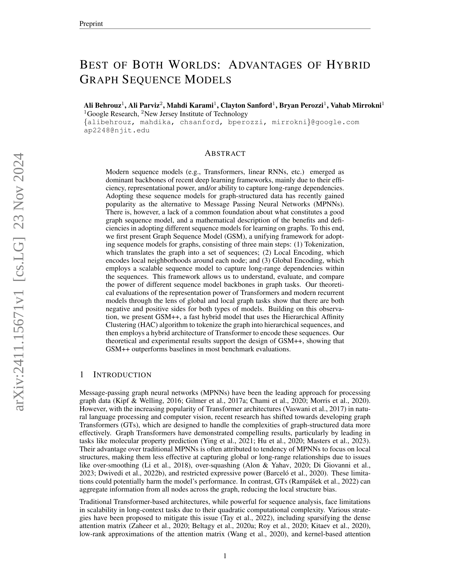
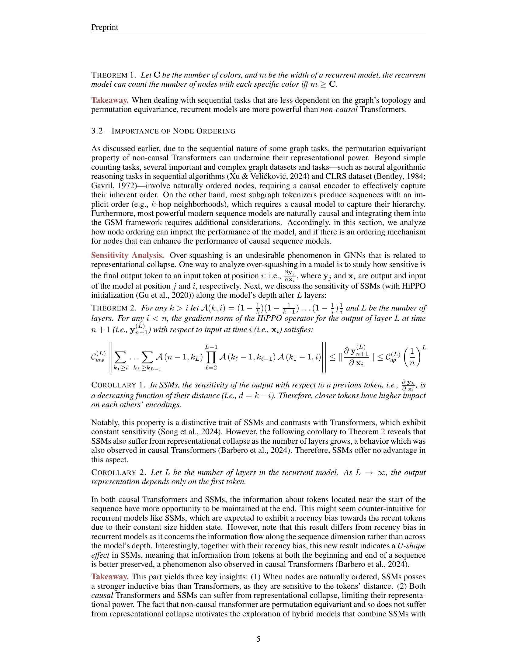
🔼 The figure illustrates the Graph Sequence Model (GSM), a framework for applying sequence models to graph data. GSM comprises three main stages: Tokenization, which converts graph data into sequences; Local Encoding, which processes local graph structures; and Global Encoding, which utilizes sequence models like RNNs or Transformers to capture long-range dependencies within sequences. The figure also highlights the strengths and weaknesses of different tokenization techniques (e.g., node vs. subgraph tokenization) and the suitability of various sequence models for specific graph tasks. Finally, the figure introduces three enhancement methods to improve GSM’s performance: Hierarchical Affinity Clustering (HAC) for improved tokenization, a hybrid encoder combining RNNs and Transformers, and a Mixture of Tokenization (MoT) approach for adaptive encoding strategies.
read the caption
Figure 1: Overview of Graph Sequence Model (GSM). GSM Consists of three stages: (1) Tokenization, (2) Local Encoding, and (3) Global Encoding. We provide a foundation for strengths and weaknesses of different tokenizations and sequence models. Finally, we present three methods to enhance the power of GSMs.
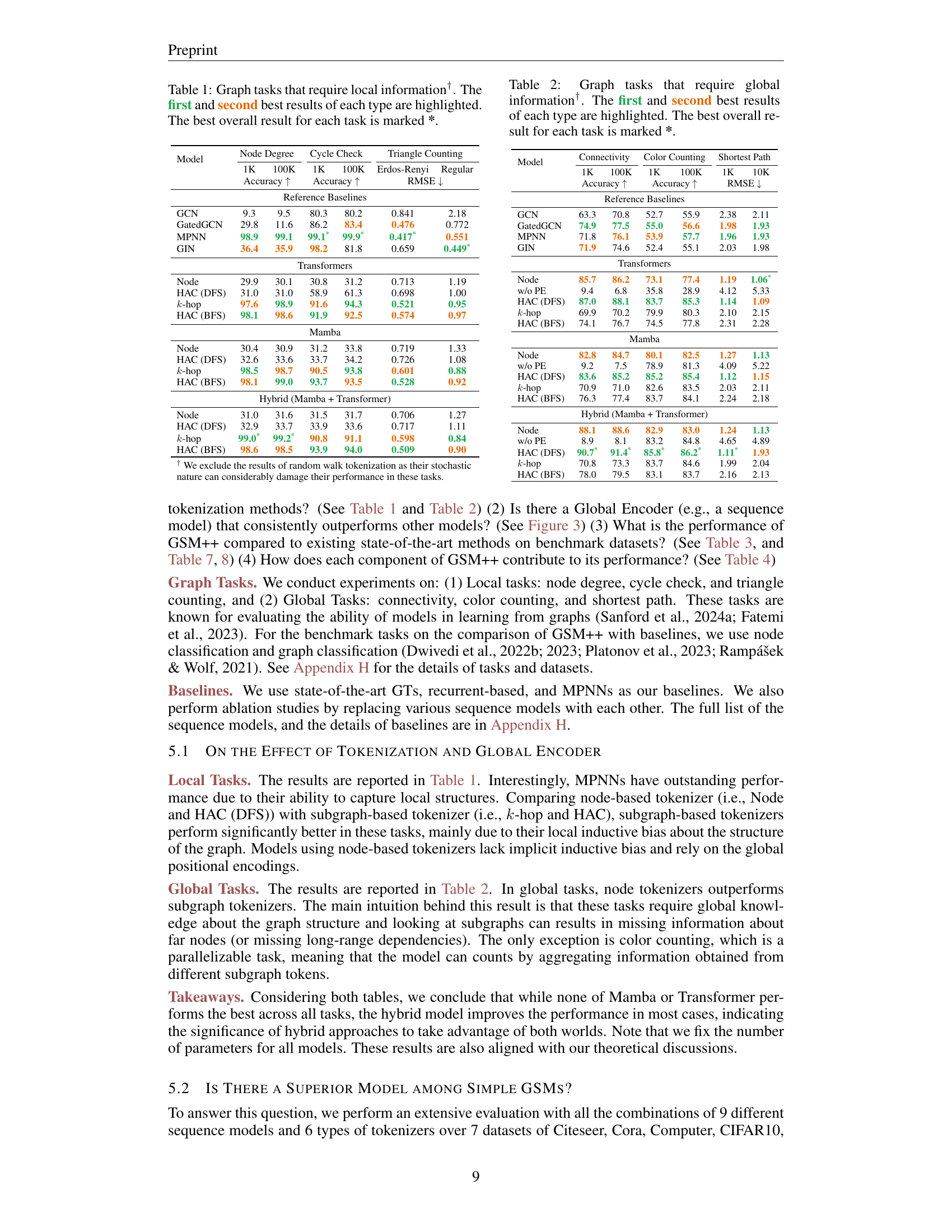
| Model | Node Degree | Node Degree | Cycle Check | Cycle Check | Triangle Counting | Triangle Counting |
|---|---|---|---|---|---|---|
| 1K | 100K | 1K | 100K | Erdos-Renyi | Regular | |
| Accuracy ↑ | Accuracy ↑ | RMSE ↓ | ||||
| Reference Baselines | ||||||
| GCN | 9.3 | 9.5 | 80.3 | 80.2 | 0.841 | 2.18 |
| GatedGCN | 29.8 | 11.6 | 86.2 | 83.4 | 0.476 | 0.772 |
| MPNN | 98.9 | 99.1 | 99.1* | 99.9* | 0.417* | 0.551 |
| GIN | 36.4 | 35.9 | 98.2 | 81.8 | 0.659 | 0.449* |
| Transformers | ||||||
| Node | 29.9 | 30.1 | 30.8 | 31.2 | 0.713 | 1.19 |
| HAC (DFS) | 31.0 | 31.0 | 58.9 | 61.3 | 0.698 | 1.00 |
| k-hop | 97.6 | 98.9 | 91.6 | 94.3 | 0.521 | 0.95 |
| HAC (BFS) | 98.1 | 98.6 | 91.9 | 92.5 | 0.574 | 0.97 |
| Mamba | ||||||
| Node | 30.4 | 30.9 | 31.2 | 33.8 | 0.719 | 1.33 |
| HAC (DFS) | 32.6 | 33.6 | 33.7 | 34.2 | 0.726 | 1.08 |
| k-hop | 98.5 | 98.7 | 90.5 | 93.8 | 0.601 | 0.88 |
| HAC (BFS) | 98.1 | 99.0 | 93.7 | 93.5 | 0.528 | 0.92 |
| Hybrid (Mamba + Transformer) | ||||||
| Node | 31.0 | 31.6 | 31.5 | 31.7 | 0.706 | 1.27 |
| HAC (DFS) | 32.9 | 33.7 | 33.9 | 33.6 | 0.717 | 1.11 |
| k-hop | 99.0* | 99.2* | 90.8 | 91.1 | 0.598 | 0.84 |
| HAC (BFS) | 98.6 | 98.5 | 93.9 | 94.0 | 0.509 | 0.90 |
🔼 This table presents the results of different graph neural network models on tasks that primarily require local information processing. The tasks include node degree prediction, cycle detection, and triangle counting. For each task, the table shows the accuracy achieved by various models on graphs with 1000 and 100,000 nodes. The best performing models for each task and dataset size are highlighted, indicating superior performance on these specific graph structures and scales. The overall best-performing model across all three tasks is marked with an asterisk (*). The symbol † indicates that the results of random walk tokenization are excluded from the table due to their stochastic nature, which can significantly impact their performance on these specific tasks.
read the caption
Table 1: Graph tasks that require local information†. The first and second best results of each type are highlighted. The best overall result for each task is marked *.
In-depth insights#
GSM Framework#
The GSM (Graph Sequence Model) framework offers a novel approach to graph representation learning by bridging the gap between sequence models and graph-structured data. Its core strength lies in its unified three-stage process: 1) Tokenization, converting the graph into sequences of nodes or subgraphs; 2) Local Encoding, capturing local neighborhood information; and 3) Global Encoding, utilizing a sequence model (e.g., RNN, Transformer) to learn long-range dependencies within the sequences. This modular design allows for systematic comparison of various sequence model backbones, revealing strengths and weaknesses in different graph tasks. The framework facilitates theoretical analysis of inductive biases of various models, providing crucial insights into their effectiveness in tasks such as counting and connectivity. A key contribution is the introduction of GSM++, a hybrid model incorporating hierarchical clustering for improved tokenization and a hybrid sequence architecture, enhancing both efficiency and performance. The theoretical and experimental evaluations validate the design choices of GSM++, showcasing its superior performance compared to baselines on various benchmark tasks.
Sequence Model Power#
The power of sequence models in the context of graph neural networks hinges on their ability to capture both local and global dependencies within graph data. While traditional message-passing networks excel at local reasoning, sequence models, particularly transformers and recurrent models, offer unique advantages in capturing long-range interactions. The choice of sequence model depends on the specific task and the properties of the input graph. Transformers, with their powerful attention mechanisms, are well-suited for global tasks requiring holistic understanding of the graph structure. However, their quadratic complexity poses scalability challenges. Recurrent models, on the other hand, are more efficient for tasks involving sequential processing or when the graph possesses inherent node ordering, though they may struggle with capturing long-range dependencies effectively. Hybrid approaches, combining transformers and recurrent models, can leverage the strengths of both architectures, potentially leading to improved performance on a wider range of tasks. The success of any sequence model is also critically dependent on the employed tokenization strategy. Different tokenization methods (node, subgraph, hierarchical) result in sequences with varying inductive biases and affect the model’s ability to learn relevant patterns.
Hybrid GSM++#
The proposed “Hybrid GSM++” model represents a significant advancement in graph neural networks by cleverly combining the strengths of recurrent and transformer architectures. GSM++ leverages a hierarchical affinity clustering (HAC) algorithm for tokenization, creating ordered sequences of nodes that capture both local and global graph structures. This approach is particularly beneficial because it addresses the limitations of existing methods, such as the over-smoothing and over-squashing problems. The hybrid nature of the model is crucial; recurrent layers enhance local information capture, while transformer layers excel at modeling long-range dependencies, effectively capturing both the local and global properties of the graph. The incorporation of a mixture of tokenization (MoT) further enhances flexibility and efficiency, adapting the best tokenization approach for each node depending on the specific task. This nuanced combination results in a powerful, scalable model that outperforms baselines on various benchmark graph learning tasks. The theoretical analysis validating these design choices supports the experimental results, thus underpinning the robustness and potential of Hybrid GSM++ for complex graph problems.
Tokenization Methods#
Tokenization, the process of converting a graph into sequences suitable for sequence models, is crucial for effective graph representation learning. The paper explores various tokenization strategies, each with its strengths and weaknesses. Node-based tokenization, treating nodes as a simple sequence, is straightforward but lacks the structural information inherent in the graph, potentially leading to suboptimal performance. Subgraph-based tokenization, representing the graph as a collection of node neighborhoods, aims to capture local structure. However, these methods require efficient techniques to handle the variable sizes and complexities of subgraphs. The choice of tokenization significantly impacts model efficiency and performance on different tasks; Node-based methods excel for global tasks, while subgraph-based approaches are superior for local tasks. The paper proposes a novel Hierarchical Affinity Clustering (HAC) based tokenization. HAC builds a hierarchical representation of the graph by recursively merging similar nodes, thus creating ordered sequences. This offers a balance, preserving the structural information while generating compact sequences. Finally, the idea of a Mixture of Tokenization (MoT) allows the algorithm to adaptively choose the best tokenization for each node, potentially maximizing model efficacy across diverse tasks and graph structures.
Future of GSMs#
The future of Graph Sequence Models (GSMs) is promising, given their ability to unify various sequence modeling approaches for graph data. Further research should focus on developing more sophisticated tokenization techniques that go beyond simple node or subgraph ordering, potentially incorporating advanced graph algorithms for more nuanced representations. Hybrid models, combining the strengths of recurrent and transformer architectures, seem particularly promising for balancing local and global information processing. Exploring alternative sequence models beyond Transformers and RNNs is also crucial to expand the capabilities and efficiency of GSMs. Finally, a deeper theoretical understanding of GSMs’ representational power and limitations with respect to different graph properties and tasks is needed. This would allow for more informed model design and better task-specific optimization.
More visual insights#
More on figures

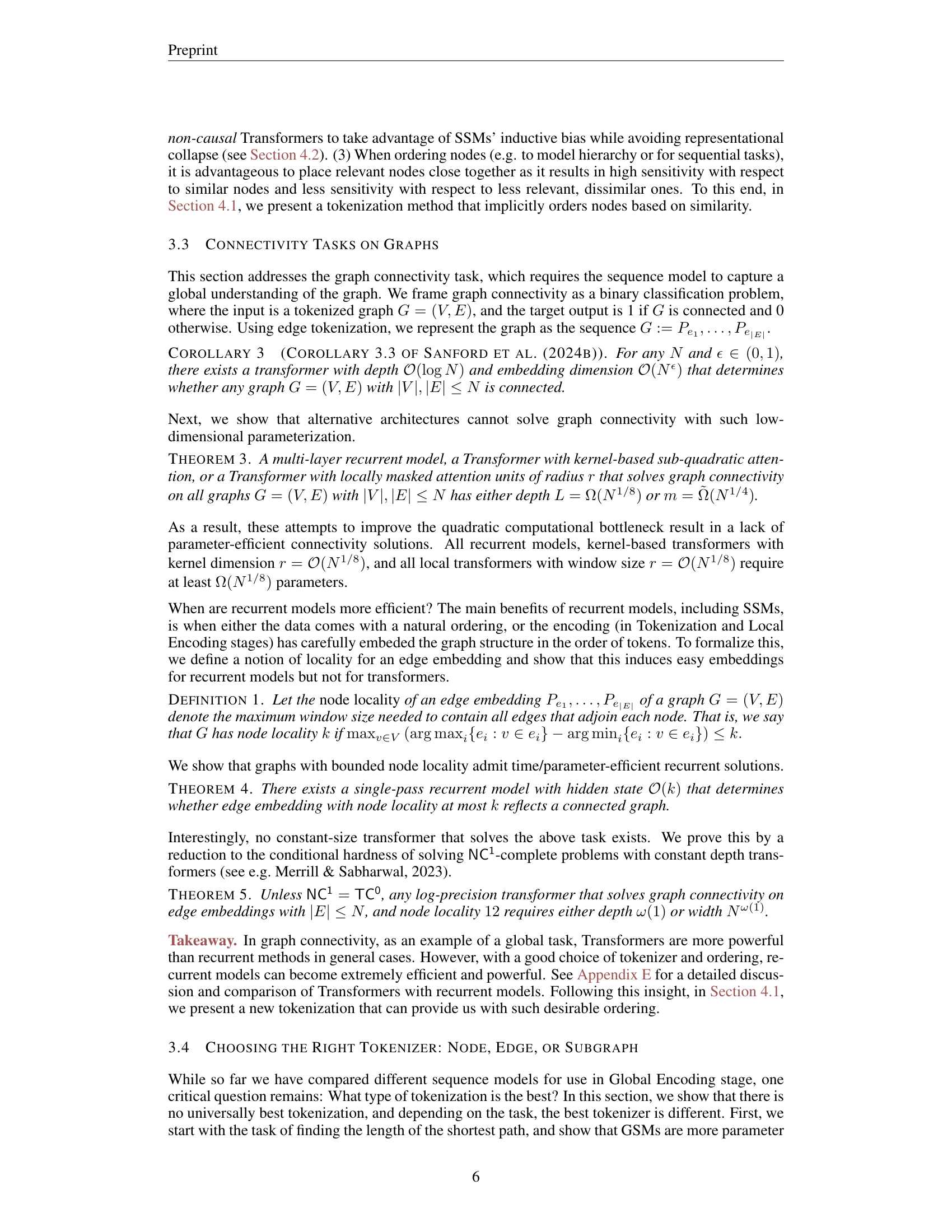
🔼 GSM++ is a model that leverages the strengths of both recurrent neural networks and transformers. It processes graph data in three stages: First, hierarchical affinity clustering (HAC) is used for tokenization, creating a hierarchical sequence representation of the graph. Second, a local encoding step captures local graph characteristics. Finally, a hybrid global encoding (using both recurrent and transformer architectures) processes the sequences, combining the ability of recurrent networks to handle sequential data effectively and the capability of transformers to capture long-range dependencies. This hybrid approach aims to overcome limitations of solely using either recurrent networks or transformers for graph-based tasks.
read the caption
Figure 2: Overview of GSM++. GSM++ is a special instance of GSMs that uses: (1) HAC tokenization, (2) hierarchical PE, and (3) a hybrid sequence model.

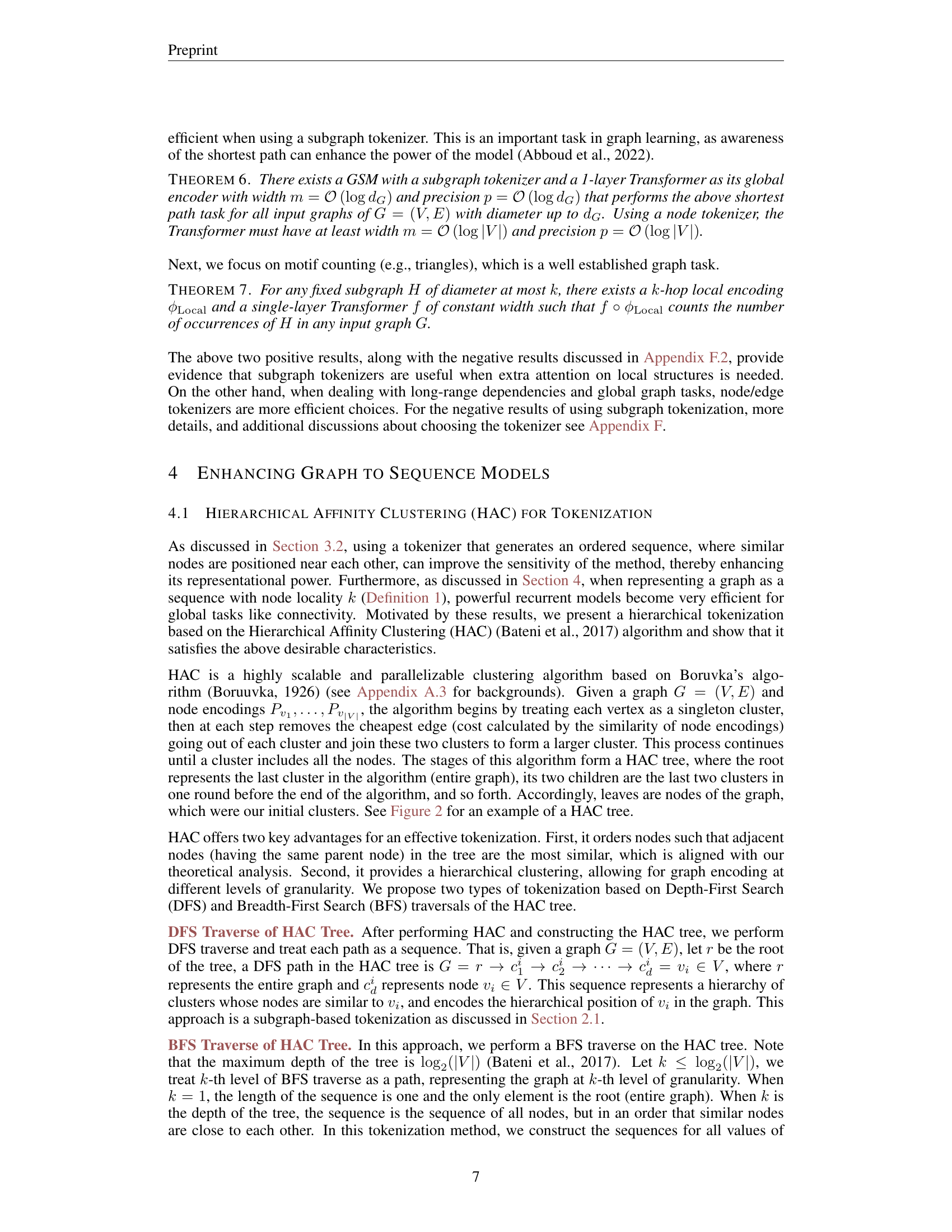
🔼 This figure visualizes the performance of various combinations of tokenization methods and global encoder (sequence model) architectures on seven benchmark graph datasets. Each cell in the heatmap represents the normalized performance score for a specific combination. The color intensity indicates the ranking, with darker shades representing higher ranks. The figure demonstrates that no single combination consistently outperforms others across all datasets, highlighting the task-dependent nature of optimal model choices. The caption notes that even the strong combination of TTT (a sequence model) and HAC (Hierarchical Affinity Clustering for tokenization) only achieves a top-3 ranking in three out of the seven datasets.
read the caption
Figure 3: Normalized score of different combination of tokenization and global encoder (sequence models). Even TTT + HAC is in Top-3 only in 3/7 datasets.
More on tables
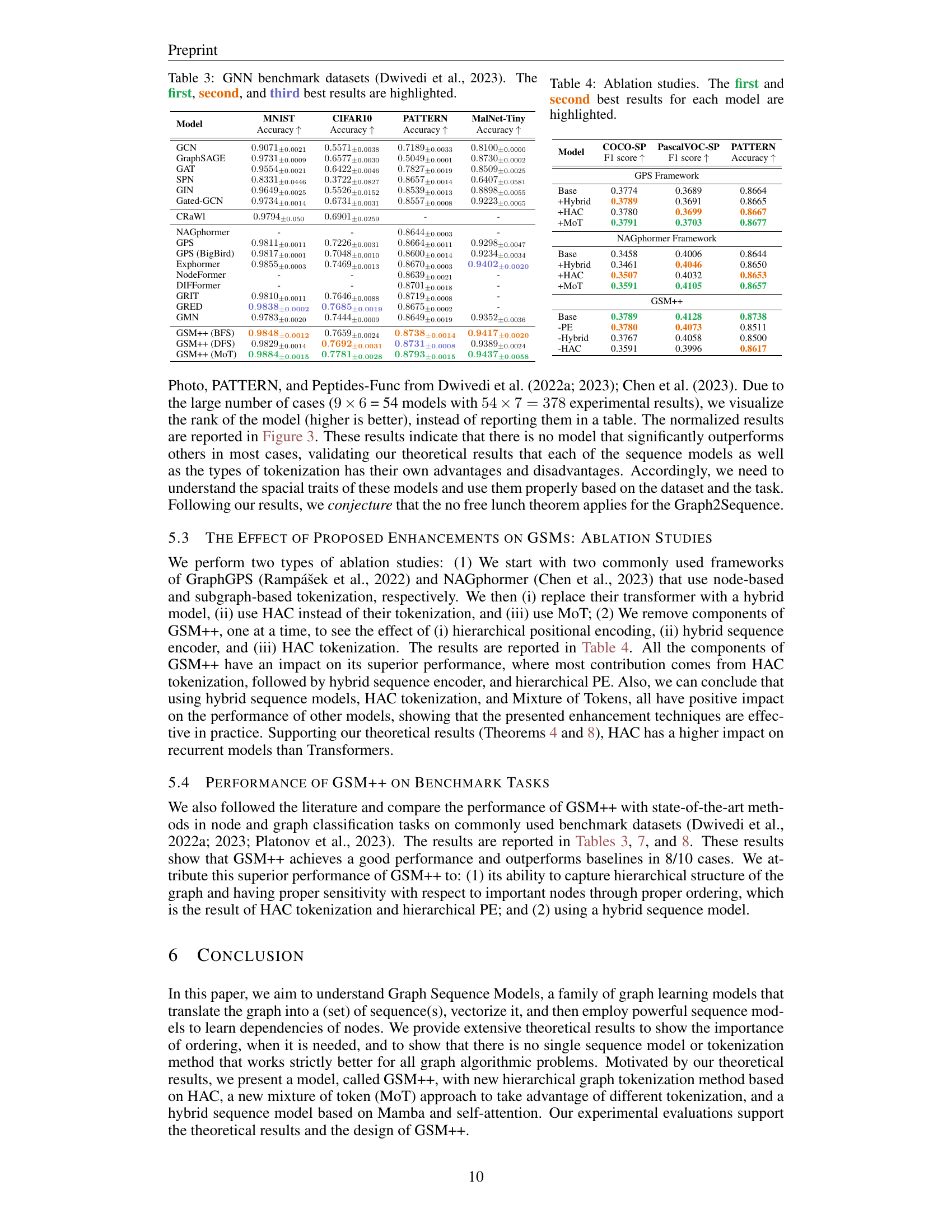
| Model | Connectivity | Color Counting | Shortest Path | |||
|---|---|---|---|---|---|---|
| 1K | 100K | 1K | 100K | 1K | 10K | |
| Reference Baselines | Accuracy ↑ | Accuracy ↑ | RMSE ↓ | |||
| GCN | 63.3 | 70.8 | 52.7 | 55.9 | 2.38 | 2.11 |
| GatedGCN | 74.9 | 77.5 | 55.0 | 56.6 | 1.98 | 1.93 |
| MPNN | 71.8 | 76.1 | 53.9 | 57.7 | 1.96 | 1.93 |
| GIN | 71.9 | 74.6 | 52.4 | 55.1 | 2.03 | 1.98 |
| Transformers | ||||||
| Node | 85.7 | 86.2 | 73.1 | 77.4 | 1.19 | 1.06* |
| w/o PE | 9.4 | 6.8 | 35.8 | 28.9 | 4.12 | 5.33 |
| HAC (DFS) | 87.0 | 88.1 | 83.7 | 85.3 | 1.14 | 1.09 |
| k-hop | 69.9 | 70.2 | 79.9 | 80.3 | 2.10 | 2.15 |
| HAC (BFS) | 74.1 | 76.7 | 74.5 | 77.8 | 2.31 | 2.28 |
| Mamba | ||||||
| Node | 82.8 | 84.7 | 80.1 | 82.5 | 1.27 | 1.13 |
| w/o PE | 9.2 | 7.5 | 78.9 | 81.3 | 4.09 | 5.22 |
| HAC (DFS) | 83.6 | 85.2 | 85.2 | 85.4 | 1.12 | 1.15 |
| k-hop | 70.9 | 71.0 | 82.6 | 83.5 | 2.03 | 2.11 |
| HAC (BFS) | 76.3 | 77.4 | 83.7 | 84.1 | 2.24 | 2.18 |
| Hybrid (Mamba + Transformer) | ||||||
| Node | 88.1 | 88.6 | 82.9 | 83.0 | 1.24 | 1.13 |
| w/o PE | 8.9 | 8.1 | 83.2 | 84.8 | 4.65 | 4.89 |
| HAC (DFS) | 90.7* | 91.4* | 85.8* | 86.2* | 1.11* | 1.93 |
| k-hop | 70.8 | 73.3 | 83.7 | 84.6 | 1.99 | 2.04 |
| HAC (BFS) | 78.0 | 79.5 | 83.1 | 83.7 | 2.16 | 2.13 |
🔼 This table presents the results of various graph tasks that necessitate global information processing. The tasks are: graph connectivity (binary classification), color counting (counting the number of nodes with each color), and shortest path (predicting shortest path lengths). For each task, multiple models were tested, and their performance is ranked, with the top two results for each task highlighted. The overall best-performing model for each task is marked with an asterisk (*). The table aims to illustrate how different model architectures handle graph problems that require considering the overall graph structure, rather than just local neighborhoods.
read the caption
Table 2: Graph tasks that require global information†. The first and second best results of each type are highlighted. The best overall result for each task is marked *.
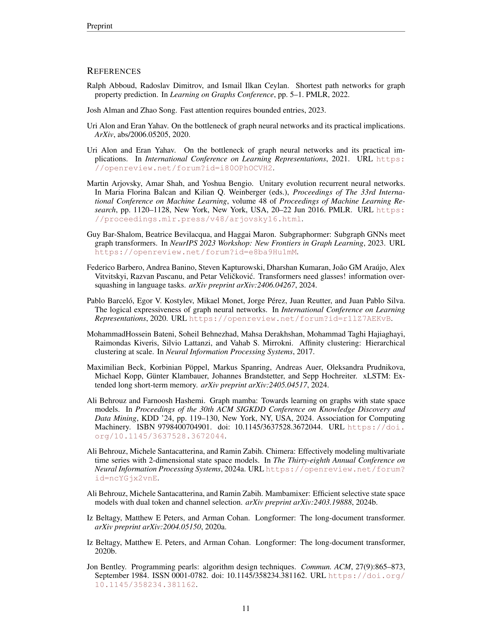
| Model | MNIST | CIFAR10 | PATTERN | MalNet-Tiny |
|---|---|---|---|---|
| GCN | 0.9071±0.0021 | 0.5571±0.0038 | 0.7189±0.0033 | 0.8100±0.0000 |
| GraphSAGE | 0.9731±0.0009 | 0.6577±0.0030 | 0.5049±0.0001 | 0.8730±0.0002 |
| GAT | 0.9554±0.0021 | 0.6422±0.0046 | 0.7827±0.0019 | 0.8509±0.0025 |
| SPN | 0.8331±0.0446 | 0.3722±0.0827 | 0.8657±0.0014 | 0.6407±0.0581 |
| GIN | 0.9649±0.0025 | 0.5526±0.0152 | 0.8539±0.0013 | 0.8898±0.0055 |
| Gated-GCN | 0.9734±0.0014 | 0.6731±0.0031 | 0.8557±0.0008 | 0.9223±0.0065 |
| CRaWl | 0.9794±0.050 | 0.6901±0.0259 | - | - |
| NAGphormer | - | - | 0.8644±0.0003 | - |
| GPS | 0.9811±0.0011 | 0.7226±0.0031 | 0.8664±0.0011 | 0.9298±0.0047 |
| GPS (BigBird) | 0.9817±0.0001 | 0.7048±0.0010 | 0.8600±0.0014 | 0.9234±0.0034 |
| Exphormer | 0.9855±0.0003 | 0.7469±0.0013 | 0.8670±0.0003 | 0.9402±0.0020 |
| NodeFormer | - | - | 0.8639±0.0021 | - |
| DIFFormer | - | - | 0.8701±0.0018 | - |
| GRIT | 0.9810±0.0011 | 0.7646±0.0088 | 0.8719±0.0008 | - |
| GRED | 0.9838±0.0002 | 0.7685±0.0019 | 0.8675±0.0002 | - |
| GMN | 0.9783±0.0020 | 0.7444±0.0009 | 0.8649±0.0019 | 0.9352±0.0036 |
| GSM++ (BFS) | 0.9848±0.0012 | 0.7659±0.0024 | 0.8738±0.0014 | 0.9417±0.0020 |
| GSM++ (DFS) | 0.9829±0.0014 | 0.7692±0.0031 | 0.8731±0.0008 | 0.9389±0.0024 |
| GSM++ (MoT) | 0.9884±0.0015 | 0.7781±0.0028 | 0.8793±0.0015 | 0.9437±0.0058 |
🔼 Table 3 presents the results of GNN benchmark datasets from Dwivedi et al. (2023). It shows a comparison of different graph neural network models’ performance on various node and graph classification tasks using four benchmark datasets: MNIST, CIFAR10, and the PATTERN and Peptides-Func datasets. The table highlights the top three performing models for each dataset and task, providing a quantitative comparison of their accuracy.
read the caption
Table 3: GNN benchmark datasets (Dwivedi et al., 2023). The first, second, and third best results are highlighted.
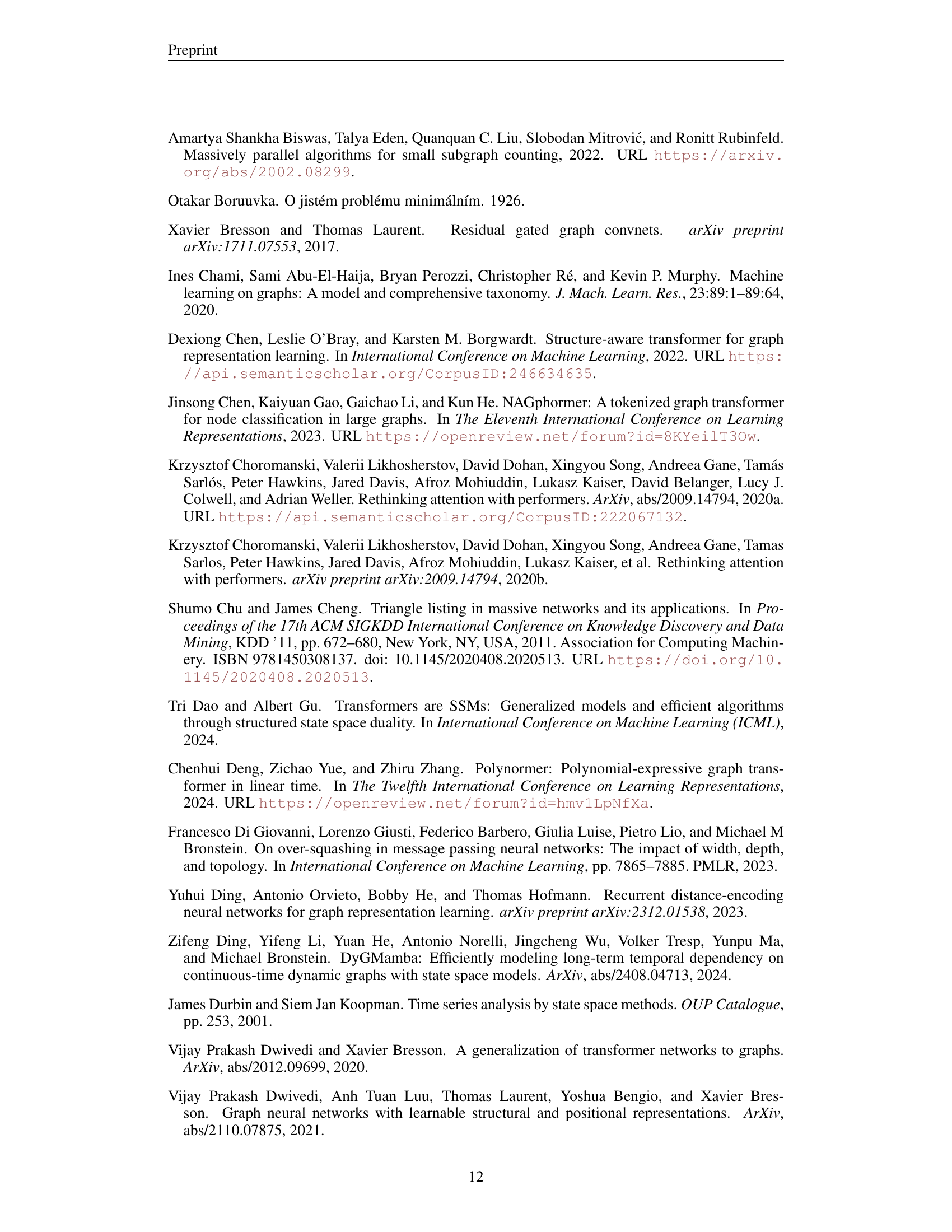
| Model | COCO-SP F1 score ↑ | PascalVOC-SP F1 score ↑ | PATTERN Accuracy ↑ |
|---|---|---|---|
| GPS Framework | |||
| Base | 0.3774 | 0.3689 | 0.8664 |
| +Hybrid | 0.3789 | 0.3691 | 0.8665 |
| +HAC | 0.3780 | 0.3699 | 0.8667 |
| +MoT | 0.3791 | 0.3703 | 0.8677 |
| NAGphormer Framework | |||
| Base | 0.3458 | 0.4006 | 0.8644 |
| +Hybrid | 0.3461 | 0.4046 | 0.8650 |
| +HAC | 0.3507 | 0.4032 | 0.8653 |
| +MoT | 0.3591 | 0.4105 | 0.8657 |
| GSM++ | |||
| Base | 0.3789 | 0.4128 | 0.8738 |
| -PE | 0.3780 | 0.4073 | 0.8511 |
| -Hybrid | 0.3767 | 0.4058 | 0.8500 |
| -HAC | 0.3591 | 0.3996 | 0.8617 |
🔼 This table presents the results of ablation studies conducted on the GSM++ model. It shows the impact of removing different components of the model (e.g., the hybrid encoder, hierarchical positional encoding, HAC tokenization, and MoT) on the overall performance. By comparing the performance metrics (F1 score and accuracy) obtained with the full model against those obtained with variations of the model where components were removed, this table helps determine the contribution of each component to the model’s overall effectiveness and efficiency.
read the caption
Table 4: Ablation studies. The first and second best results for each model are highlighted.
| Method | Tokenization | Local Encoding | Global Encoding |
|---|---|---|---|
| DeepWalk (2014) | Random Walk | Identity(.) | SkipGram |
| Node2Vec (2016) | 2nd Order Random Walk | Identity(.) | SkipGram |
| Node2Vec (2016) | Random Walk | Identity(.) | SkipGram |
| GraphTransformer (2020) | Node | Identity(.) | Transformer |
| GraphGPS (2022) | Node | Identity(.) | Transformer |
| NodeFormer (2022) | Node | Gumbel-Softmax(.) | Transformer |
| Graph-ViT (2023) | METIS Clustering (Patching) | Gcn(.) | ViT |
| Exphormer (2023) | Node | Identity(.) | Sparse Transformer |
| CRaWl (2023) | Random Walk | 1D Convolutions | MLP(.) |
| NAGphormer (2023) | k-hop neighborhoods | Gcn(.) | Transformer |
| SP-MPNNs (2022) | k-hop neighborhoods | Identity(.) | GIN(.) |
| GRED (2023) | k-hop neighborhood | MLP(.) | Rnn(.) |
| S4G (2024) | k-hop neighborhood | Identity(.) | S4(.) |
| Graph Mamba (2024) | Union of Random Walks (With varying length) | Gated-Gcn(.) | Bi-Mamba(.) |
🔼 This table shows how various graph neural network models can be viewed as special cases of the general Graph Sequence Model (GSM) framework proposed in the paper. For each model, the table lists the tokenization method used to convert the graph into sequences (e.g., node-based, subgraph-based), the local encoding technique applied to each token (e.g., identity, GCN), and the global encoding model used to capture long-range dependencies (e.g., SkipGram, Transformer, RNN). This allows for a systematic comparison of different model architectures and highlights the common underlying principles across these models.
read the caption
Table 5: How are different models special instances of GSM framework
| Dataset | #Graphs | Average #Nodes | Average #Edges | #Class | Input Level | Task | Metric |
|---|---|---|---|---|---|---|---|
| Long-range Graph Benchmark (Dwivedi et al., 2022a) | |||||||
| COCO-SP | 123,286 | 476.9 | 2693.7 | 81 | Node | Classification | F1 score |
| PascalVOC-SP | 11,355 | 479.4 | 2710.5 | 21 | Node | Classification | F1 score |
| Peptides-Func | 15,535 | 150.9 | 307.3 | 10 | Graph | Classification | Average Precision |
| Peptides-Struct | 15,535 | 150.9 | 307.3 | 11 (regression) | Graph | Regression | Mean Absolute Error |
| GNN Benchmark (Dwivedi et al., 2023) | |||||||
| Pattern | 14,000 | 118.9 | 3,039.3 | 2 | Node | Classification | Accuracy |
| MNIST | 70,000 | 70.6 | 564.5 | 10 | Graph | Classification | Accuracy |
| CIFAR10 | 60,000 | 117.6 | 941.1 | 10 | Graph | Classification | Accuracy |
| MalNet-Tiny | 5,000 | 1,410.3 | 2,859.9 | 5 | Graph | Classification | Accuracy |
| Heterophilic Benchmark (Platonov et al., 2023) | |||||||
| Roman-empire | 1 | 22,662 | 32,927 | 18 | Node | Classification | Accuracy |
| Amazon-ratings | 1 | 24,492 | 93,050 | 5 | Node | Classification | Accuracy |
| Minesweeper | 1 | 10,000 | 39,402 | 2 | Node | Classification | ROC AUC |
| Tolokers | 1 | 11,758 | 519,000 | 2 | Node | Classification | ROC AUC |
| Very Large Dataset (Hu et al., 2020) | |||||||
| arXiv-ogbn | 1 | 169,343 | 1,166,243 | 40 | Node | Classification | Accuracy |
| products-ogbn | 1 | 2,449,029 | 61,859,140 | 47 | Node | Classification | Accuracy |
| Color-connectivty task (Rampášek & Wolf, 2021) | |||||||
| C-C 16x16 grid | 15,000 | 256 | 480 | 2 | Node | Classification | Accuracy |
| C-C 32x32 grid | 15,000 | 1,024 | 1,984 | 2 | Node | Classification | Accuracy |
| C-C Euroroad | 15,000 | 1,174 | 1,417 | 2 | Node | Classification | Accuracy |
| C-C Minnesota | 6,000 | 2,642 | 3,304 | 2 | Node | Classification | Accuracy |
🔼 This table presents a comprehensive overview of the datasets used in the experiments. For each dataset, it lists key statistics, including the number of graphs, the average number of nodes and edges per graph, the experimental setup (e.g., node classification, graph classification), the number of classes for classification tasks, and the specific evaluation metric used (e.g., accuracy, F1-score, AUC). The datasets are categorized into those designed for long-range dependencies, heterophily, and those focused on specific tasks like color connectivity.
read the caption
Table 6: Dataset Statistics.
🔼 This table presents the results of different graph neural network models on three heterophilic graph datasets: Roman-empire, Amazon-ratings, and Minesweeper. Heterophilic graphs are those where nodes within the same class have diverse features, making them challenging for graph neural networks to learn. The table shows the accuracy, F1-score, and ROC AUC (Area Under the Curve) achieved by each model on each dataset. The top three performing models for each metric are highlighted to facilitate comparison and identification of the best-performing models for each dataset and task.
read the caption
Table 7: Heterophilic datasets (Platonov et al., 2023). The first, second, and third results are highlighted.
🔼 This table presents the results of various graph neural network models on three benchmark datasets: COCO-SP, PascalVOC-SP, and Peptides-Func. These datasets are characterized by long-range dependencies between nodes, making them challenging for many graph models. The table shows the performance of each model on each dataset, measured by F1 score (for COCO-SP and PascalVOC-SP) and Average Precision (for Peptides-Func). The top three performing models for each dataset are highlighted to illustrate the relative strengths and weaknesses of different approaches for handling long-range graph dependencies.
read the caption
Table 8: Long-Range Datasets (Dwivedi et al., 2022a). The first, second, and third results are highlighted.
| Model | GatedGCN | NAGphormer | GPS | Exphormer | GOAT | GRIT | GMN | GSM++ BFS | GSM++ DFS | GSM++ MoT |
|---|---|---|---|---|---|---|---|---|---|---|
| arXiv-ogbn Performance | 0.7141 | 0.7013 | OOM | 0.7228 | 0.7196 | OOM | 0.7248 | 0.7297 | 0.7261 | 0.7301 |
| arXiv-ogbn Memory Usage (GB) | 11.87 | 6.81 | OOM | 37.01 | 13.12 | OOM | 5.63 | 24.8 | 4.7 | 14.9 |
| arXiv-ogbn Training Time/Epoch (s) | 1.94 | 5.96 | OOM | 2.15 | 8.69 | OOM | 1.78 | 2.33 | 1.95 | 4.16 |
| products-ogbn Performance | 0.0000 | 0.0000 | OOM | OOM | 0.8200 | OOM | OOM | 0.8071 | 0.8080 | 0.8213 |
| products-ogbn Memory Usage (GB) | 11.13 | 10.04 | OOM | OOM | 12.06 | OOM | OOM | 38.14 | 9.15 | 11.96 |
| products-ogbn Training Time/Epoch (s) | 1.92 | 12.08 | OOM | OOM | 29.50 | OOM | OOM | 6.97 | 12.19 | 11.87 |
🔼 This table presents a comparison of the performance of various graph neural network models on two large graph datasets: arXiv-ogbn and products-ogbn. The metrics evaluated include accuracy (Performance), memory usage (Memory Usage (GB)), and training time per epoch (Training Time/Epoch (s)). The models compared encompass several state-of-the-art Graph Transformers and a novel hybrid model called GSM++. The table highlights the top three performing models for each metric. ‘OOM’ indicates that the model ran out of memory and could not complete training.
read the caption
Table 9: Efficiency evaluation on large graphs. The first, second, and third results for each metric are highlighted. OOM: Out of memory.
Full paper#
