↗ arXiv ↗ Hugging Face ↗ Papers with Code
TL;DR#
Large language models (LLMs) sometimes exhibit surprising new capabilities as they grow larger, a phenomenon known as ’emergence’. This poses a challenge for researchers because it’s difficult to predict when and how these capabilities will appear. The paper tackles this challenge. It highlights the difficulty in anticipating emergent capabilities in LLMs due to the unpredictability of downstream capabilities despite predictable pretraining loss. This difficulty impacts model developers, policymakers, and stakeholders who make decisions based on future LLM capabilities.
The researchers propose a novel approach to predict LLM emergence. They found that finetuning LLMs on a specific task shifts the point at which emergence occurs towards less capable models. They operationalized this insight by finetuning LLMs with varying data amounts and fitting a parametric function to predict emergence. Their method successfully predicted emergence using only smaller-scale LLMs, showing promise in forecasting capabilities of models trained with up to 4x more compute. They also demonstrated practical uses for their method in assessing data quality and anticipating future LLM capabilities.
Key Takeaways#
Why does it matter?#
This paper is crucial for researchers working with large language models (LLMs). It introduces a novel method for predicting the emergence of capabilities in LLMs, which is a significant challenge in the field. This allows for better resource allocation and safer development of future LLMs by anticipating capabilities and potential risks before they emerge, enabling proactive risk management. The proposed method is also valuable for improving data quality assessment during LLM training.
Visual Insights#

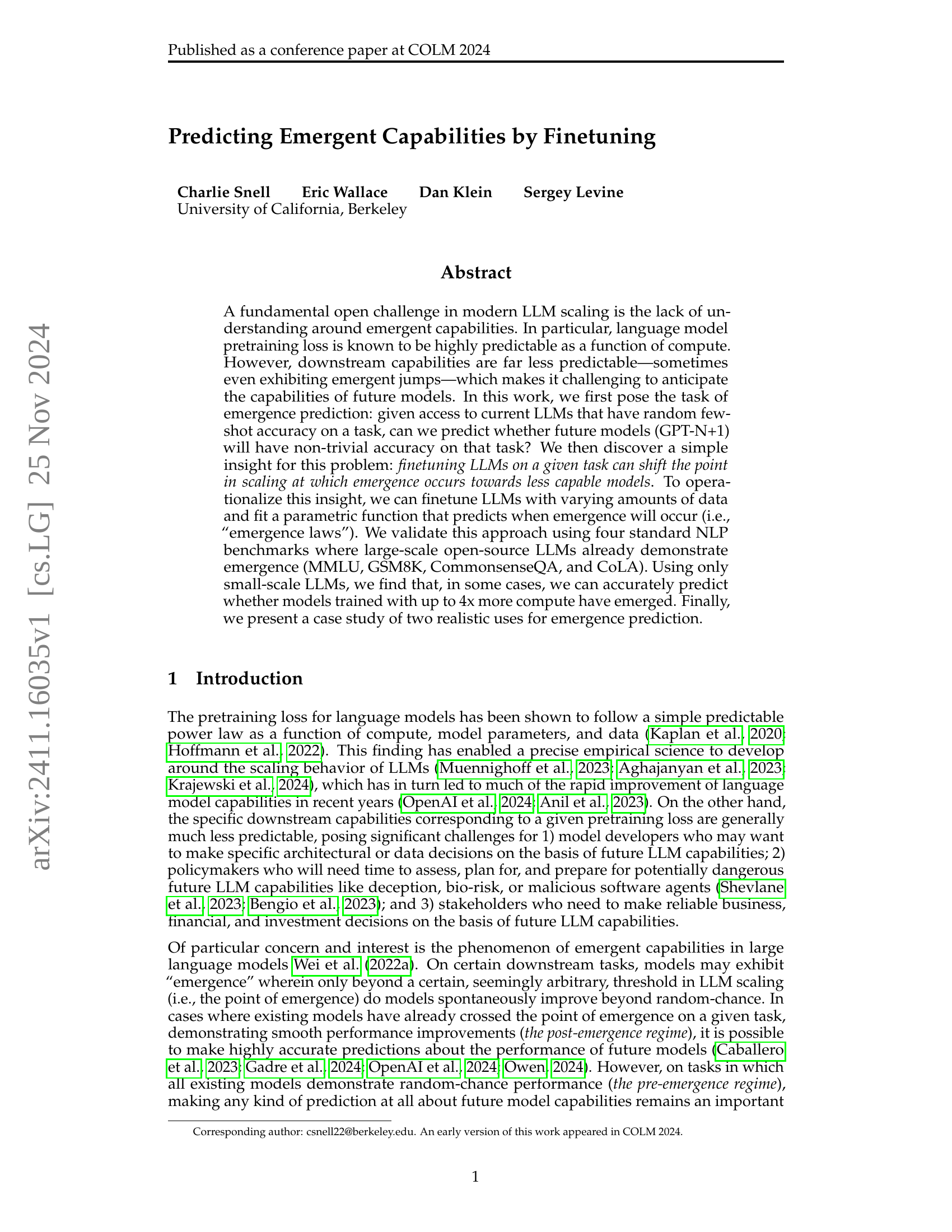
🔼 This figure illustrates the effect of finetuning on the emergence of capabilities in large language models. The left panel shows that for a specific task, finetuning a model with increasing amounts of data shifts the point at which it starts showing non-trivial performance (emergence point) towards models with lower capabilities. The right panel introduces a novel method to predict when few-shot emergence will occur. An ’emergence law’ is proposed – a parametric function that models how the emergence point shifts as a function of finetuning data. Using this law, the emergence point for few-shot learning can be predicted by extrapolating to the limit of small amounts of finetuning data. This allows researchers to anticipate the capabilities of future, larger models.
read the caption
Figure 1: We find that task-specific finetuning systematically shifts the point of emergence towards less capable models. Motivated by this finding, we develop an emergence law, which models how the point of emergence shifts as a function of the amount of finetuning data. Using this emergence law, we can then extrapolate a prediction for the point of emergence in the few-shot setting.
| Symbol | Description |
|---|---|
| Amount of finetuning data | |
| <math alttext=“L( |
text{M})” class=“ltx_Math” display=“inline” id=“S5.T1.2.2.1.m1.1”>
text{M})
theta}(D)” class=“ltx_Math” display=“inline” id=“S5.T1.6.6.1.m1.1”>
theta}(D)
alpha,C” class=“ltx_Math” display=“inline” id=“S5.T1.7.7.1.m1.3”>
alpha,C
🔼 This table lists the symbols used in Section 5 of the paper and their corresponding descriptions. It provides a key for understanding the mathematical notation and variables used in the emergence law model presented in that section. The symbols include those representing the amount of finetuning data, the model’s pretraining loss, downstream performance, and the parameters used in the emergence law itself.
read the caption
Table 1: Symbols used in Section 5.
In-depth insights#
Emergence Prediction#
The concept of ‘Emergence Prediction’ in the context of large language models (LLMs) is a significant advancement. The core idea revolves around predicting when a model will exhibit emergent capabilities on a given task, even before it reaches the necessary scale for such capabilities to manifest. This is a crucial step because emergent capabilities, while desirable, are also unpredictable and potentially dangerous. The approach detailed utilizes finetuning as a crucial tool. Finetuning smaller LLMs on a specific task systematically shifts the point of emergence to lower-capacity models, revealing insights into the data and training dynamics needed for emergence. By fitting a parametric function to these results, researchers develop ‘emergence laws’—essentially predictive models—to anticipate emergence in larger models. This process avoids the expensive process of training multiple, large-scale models to identify emergent capabilities, offering significant cost and time savings while mitigating potential risks. The validity of this approach is demonstrated via successful predictions on multiple standard NLP benchmarks, where emergence has already been observed, proving the efficacy of predicting emergence using this novel method. The ability to predict emergent capabilities in advance allows researchers and developers to make more informed decisions regarding model development, resource allocation, and safety protocols.
Finetuning Effects#
Finetuning’s impact on large language models (LLMs) is a significant area of study. The core concept is that fine-tuning systematically shifts the point of emergence, making the capabilities of less powerful models more predictable. By training smaller LLMs on a task and observing how their performance changes with varying amounts of data, researchers can fit a parametric function (an “emergence law”). This law extrapolates to the low-data limit, effectively predicting when more substantial models will exhibit emergent capabilities on the same task. The study shows that finetuning data amount directly influences the emergence point, shifting it towards weaker models with more data. This insight is crucial for predicting downstream capabilities in larger, more costly models which makes it a valuable tool for LLM development and resource allocation. Further research should investigate the underlying mechanisms driving this shift and explore the generalizability of emergence laws across different model architectures and tasks.
Emergence Laws#
The concept of “Emergence Laws” in the context of large language models (LLMs) is a significant contribution because it proposes a systematic way to predict the emergence of capabilities in future models. Instead of relying on unpredictable jumps in performance, this framework uses finetuning experiments on smaller LLMs to extrapolate how larger models will behave, effectively constructing a predictive model (the “emergence law”). This is a powerful tool because it shifts the prediction problem from the realm of highly unpredictable emergent behavior to a more manageable task of fitting a parametric function, paving the way for earlier and more accurate assessments of future LLM capabilities. The core idea is that finetuning, by shifting the point of emergence, reveals critical data on the underlying scaling behavior; thus, the law allows for predictions even with limited data, provided this data is carefully selected. The application of this approach opens possibilities for informed decision-making in LLM development; however, the validity and generalization of such laws require further investigation and validation.
Real-World Uses#
The ‘Real-World Uses’ section of this research paper explores the practical applications of the proposed emergence prediction methodology. Two key applications are highlighted: 1) evaluating the quality of pretraining data more efficiently and 2) predicting the emergence of complex capabilities in future, more powerful LLMs. The first application offers a cost-effective method for assessing data quality, avoiding the need for extensive large-scale model training. This is crucial for resource management and iterative development processes. The second application focuses on anticipating the capabilities of future models, potentially identifying dangerous or unforeseen emergent behaviors, critical for safety and responsible development. Both applications highlight the significant impact this work could have on the broader LLM development landscape by improving efficiency and enabling proactive risk mitigation strategies.
Future Directions#
The paper’s exploration of emergence prediction in large language models (LLMs) reveals a promising yet nascent field. Future directions should prioritize refining data collection strategies to improve prediction accuracy. This could involve leveraging active learning techniques to focus on the most informative data points. Addressing the mechanistic understanding of why finetuning shifts the point of emergence is crucial. Is it accelerating an underlying phase transition or merely surfacing latent capabilities? Further investigation is needed to test the generalizability of these findings to different LLM architectures and training paradigms. The current approach may not directly translate to models with significant architectural differences or those trained using alternative methods like distillation. Finally, extending the predictive capabilities to more complex, safety-relevant capabilities present in frontier LLMs remains a critical challenge. This will necessitate developing more sophisticated methods beyond simple emergence prediction, perhaps integrating interpretability techniques to gain deeper insights into the inner workings of these advanced models.
More visual insights#
More on figures

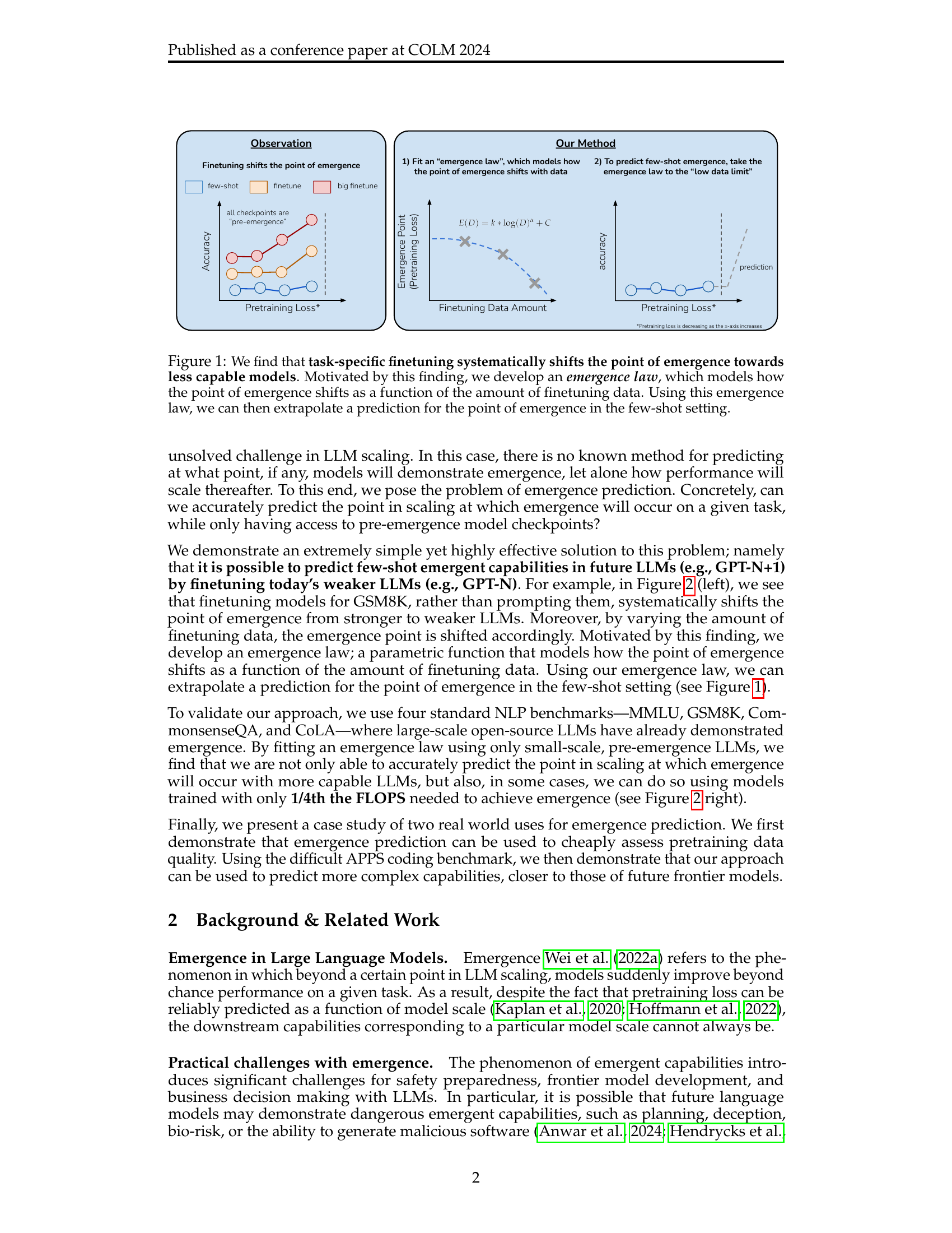
🔼 This figure demonstrates the core idea of the paper: predicting the emergence of capabilities in large language models (LLMs) by finetuning smaller, pre-emergence models. The left panel shows how finetuning shifts the point at which a capability emerges (the ’emergence point’) to lower-performing models. The more data used for finetuning, the greater this shift. By fitting a mathematical function (’emergence law’) to this relationship, the authors can extrapolate to predict when emergence will occur in larger, unseen models, even using very limited data. The right panel shows the success rate of this method, demonstrating that they can accurately predict the emergence point up to 4 times the computational resources of the models used to build the prediction.
read the caption
Figure 2: Left: we predict emergence in the few-shot setting by leveraging information about how “pre-emergence” models behave after finetuning. Our key finding is that finetuning effectively shifts the point of emergence from stronger to weaker models. Moreover, by varying the amount of finetuning data, the emergence point is shifted accordingly. We can use this finding to predict when few-shot emergence will occur by fitting a parametric function to the results (i.e., emergence law) and then taking a limit. Right: using this approach, we can predict emergence up to 4x the FLOPs in advance.

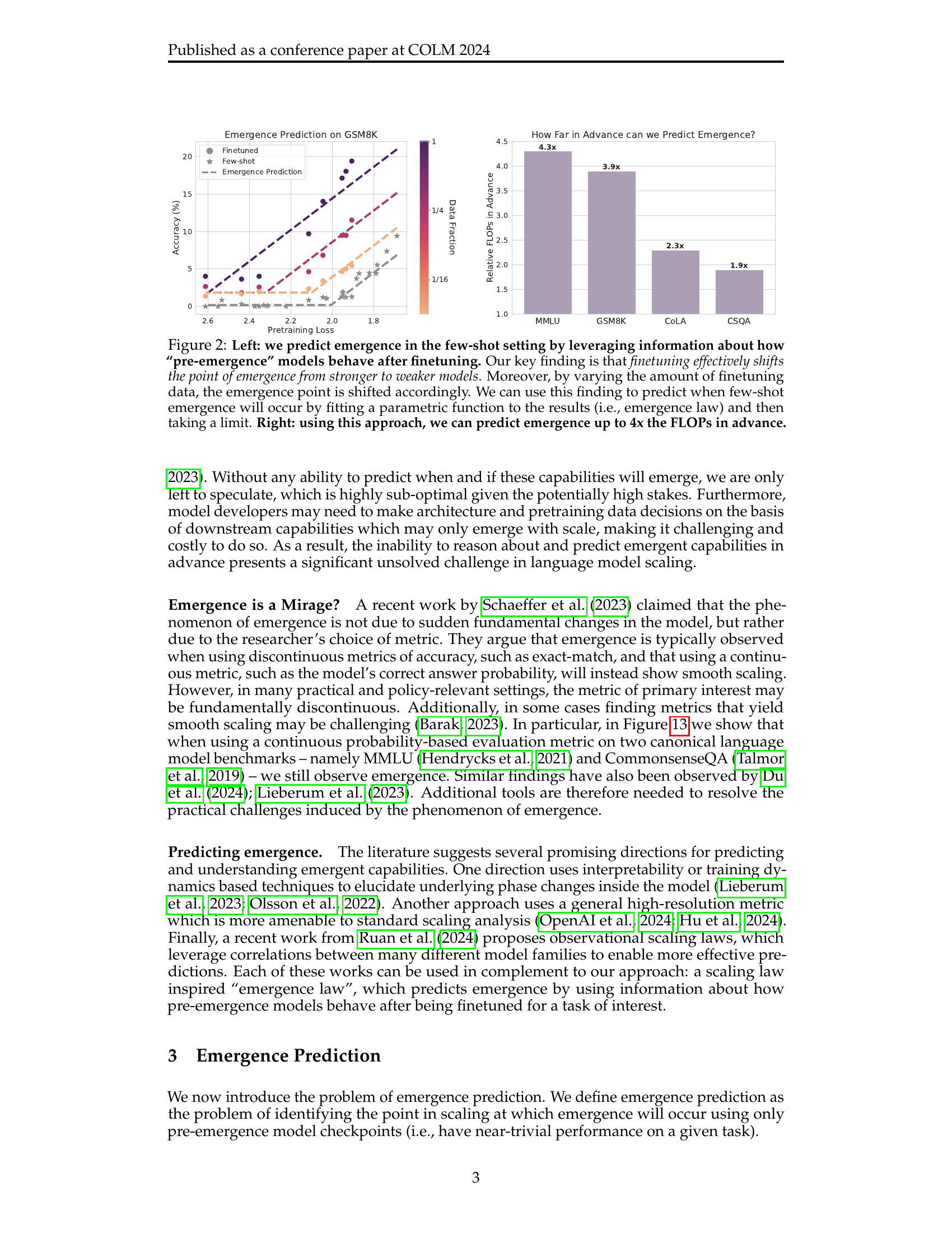
🔼 This figure shows how finetuning affects the emergence of capabilities in LLMs. The left panel plots the few-shot and finetuned performance of intermediate-sized LLMs (3B, 7B, and 13B parameters) on two tasks (MMLU and GSM8K). It demonstrates that finetuning systematically shifts the point at which a capability emerges towards less powerful models. Importantly, the degree of this shift is consistent across different model sizes at the same pretraining loss. The right panel shows how the amount of data used for finetuning further influences this shift, with more data leading to an even earlier emergence on less capable models.
read the caption
Figure 3: Left: the finetuned and few-shot performance of intermediate LLM checkpoints. We plot downstream accuracy against pretraining loss for all 3B, 7B, and 13B intermediate OpenLLaMA V1 checkpoints on MMLU and GSM8K. We see that the point of emergence is systematically shifted towards weaker LLMs after finetuning. Additionally, the magnitude of the shift is consistent across all model sizes at the same pretraining loss. Right: varying the amount of finetuning data. We finetune the 3B intermediate checkpoints on subsets of the full finetuning data. We see that as we increase the amount of finetuning data, the point of emergence shifts further towards less capable LLMs.

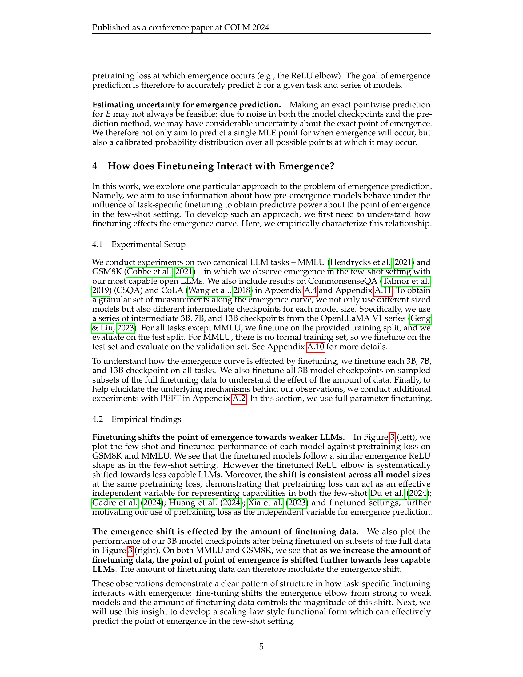
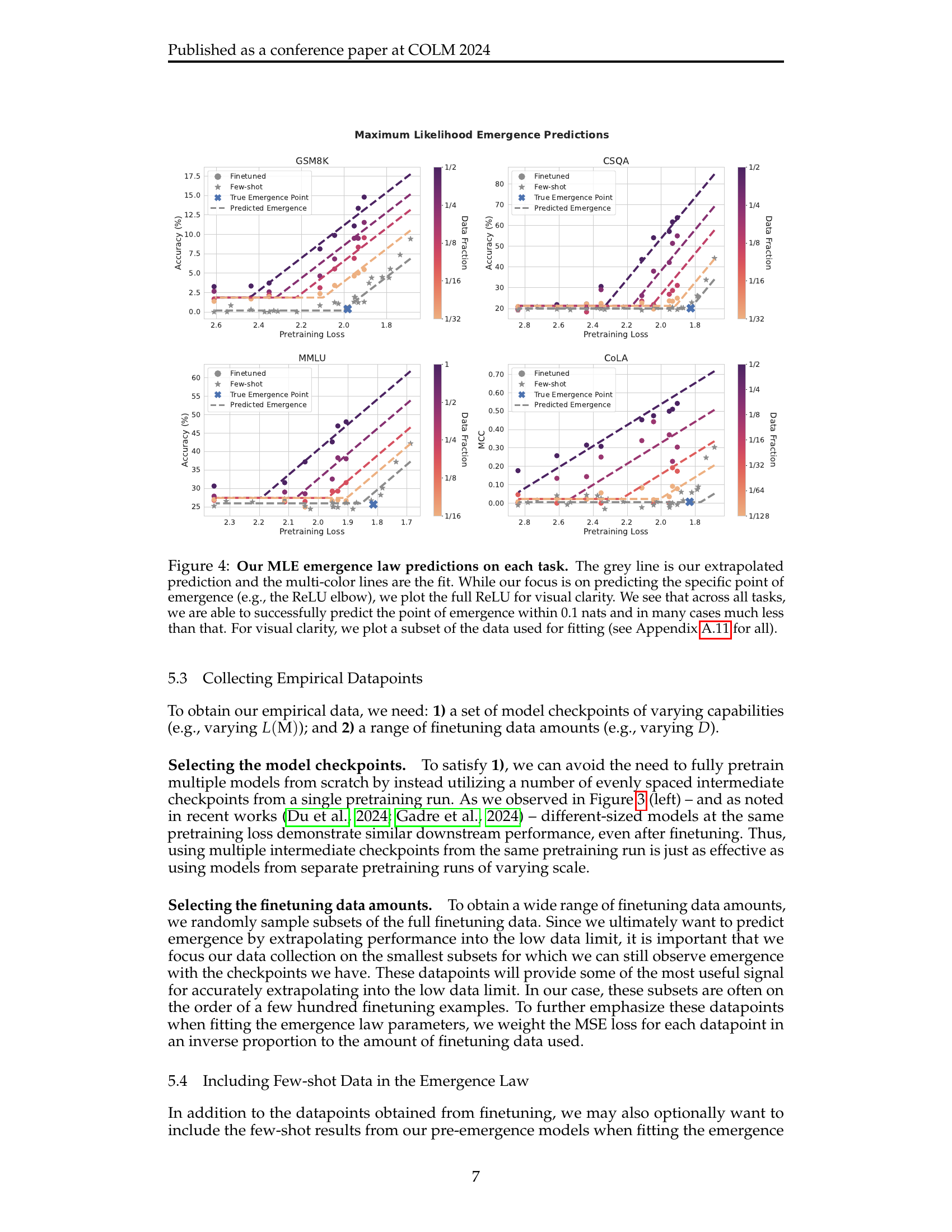
🔼 Figure 4 presents the maximum likelihood estimations of emergence points from the emergence law model. The grey line represents the extrapolated prediction of the emergence point for each task (MMLU, GSM8K, CSQA, CoLA) in a few-shot setting. The multi-colored lines show the model’s fit to the data using different amounts of finetuning data. Each colored line represents the shift in the emergence point as the amount of finetuning data changes. The figure highlights the model’s accurate predictions of the emergence points, typically within a margin of 0.1 nats, often much less. The full ReLU function is displayed for visual clarity, though the primary focus is on the precise point of emergence (the ’elbow’ of the ReLU). A subset of the data is shown for clarity; Appendix A.11 contains all data used in the model fitting.
read the caption
Figure 4: Our MLE emergence law predictions on each task. The grey line is our extrapolated prediction and the multi-color lines are the fit. While our focus is on predicting the specific point of emergence (e.g., the ReLU elbow), we plot the full ReLU for visual clarity. We see that across all tasks, we are able to successfully predict the point of emergence within 0.1 nats and in many cases much less than that. For visual clarity, we plot a subset of the data used for fitting (see Appendix A.11 for all).

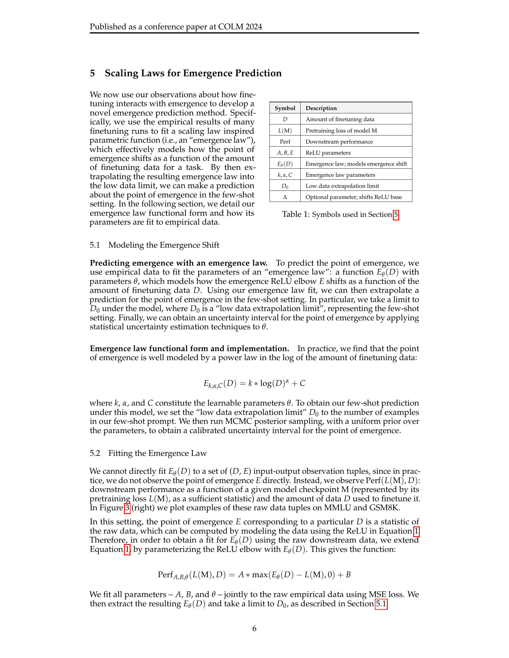
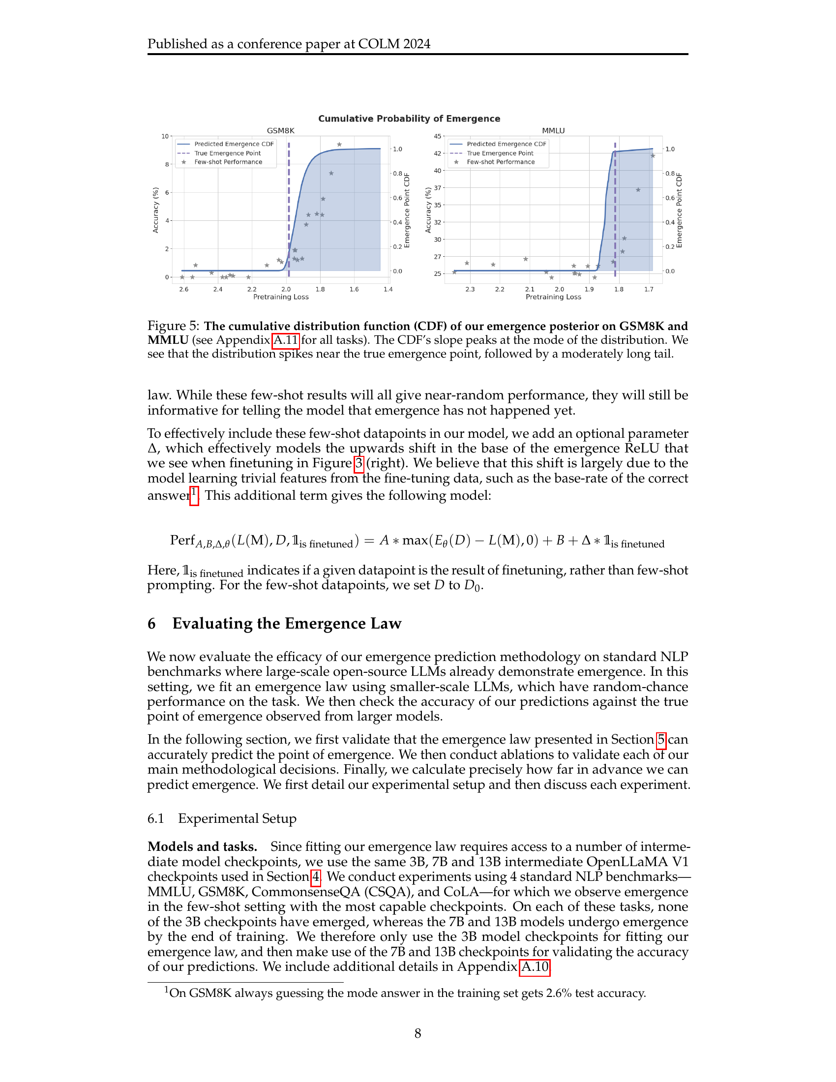
🔼 This figure displays the cumulative distribution function (CDF) plots illustrating the emergence posterior for two NLP tasks: GSM8K and MMLU. The x-axis represents the point of emergence (in terms of pretraining loss), and the y-axis shows the cumulative probability. The peak of the CDF’s slope indicates the most likely point of emergence, which is close to the actual observed point. The moderately long tail suggests uncertainty in precisely pinpointing the emergence point, implying the model’s confidence in prediction isn’t absolute but is concentrated near the actual emergence point.
read the caption
Figure 5: The cumulative distribution function (CDF) of our emergence posterior on GSM8K and MMLU (see Appendix A.11 for all tasks). The CDF’s slope peaks at the mode of the distribution. We see that the distribution spikes near the true emergence point, followed by a moderately long tail.

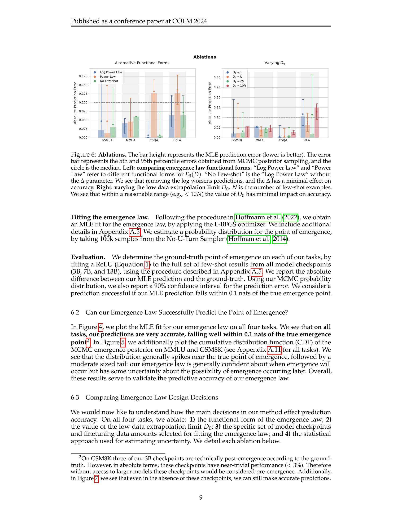
🔼 This figure presents ablation studies on the emergence prediction method. The left panel compares three different functional forms for the emergence law: a log power law, a power law, and a log power law without the delta parameter. The results show that removing the log term significantly worsens the prediction accuracy, while the delta parameter has minimal impact. The right panel investigates the effect of varying the low-data extrapolation limit (D0) on prediction accuracy. The results indicate that within a reasonable range (less than 10 times the number of few-shot examples), the choice of D0 has minimal effect on accuracy.
read the caption
Figure 6: Ablations. The bar height represents the MLE prediction error (lower is better). The error bar represents the 5th and 95th percentile errors obtained from MCMC posterior sampling, and the circle is the median. Left: comparing emergence law functional forms. “Log Power Law” and “Power Law” refer to different functional forms for Eθ(D)subscript𝐸𝜃𝐷E_{\theta}(D)italic_E start_POSTSUBSCRIPT italic_θ end_POSTSUBSCRIPT ( italic_D ). “No Few-shot” is the “Log Power Law” without the ΔΔ\Deltaroman_Δ parameter. We see that removing the log worsens predictions, and the ΔΔ\Deltaroman_Δ has a minimal effect on accuracy. Right: varying the low data extrapolation limit D0subscript𝐷0D_{0}italic_D start_POSTSUBSCRIPT 0 end_POSTSUBSCRIPT. N𝑁Nitalic_N is the number of few-shot examples. We see that within a reasonable range (e.g., <10Nabsent10𝑁<10N< 10 italic_N) the value of D0subscript𝐷0D_{0}italic_D start_POSTSUBSCRIPT 0 end_POSTSUBSCRIPT has minimal impact on accuracy.

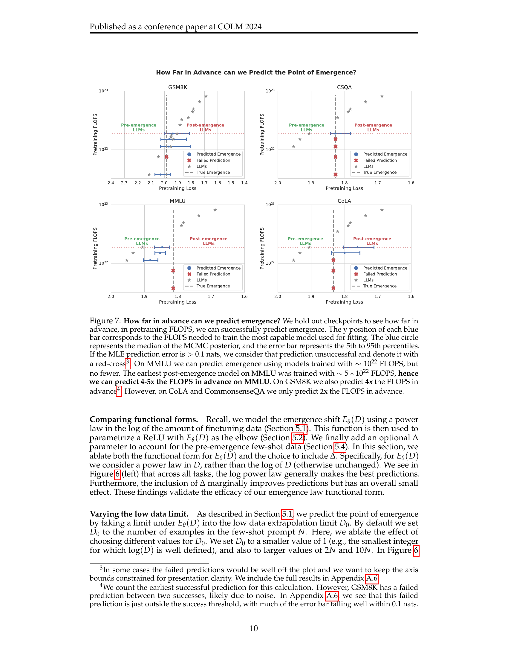
🔼 Figure 7 investigates how far in advance the proposed emergence prediction method can accurately predict the emergence point in terms of FLOPs (floating point operations). By holding out checkpoints from the model training process, the study assesses the predictive capability for various benchmarks. Each blue bar in the figure indicates the FLOPs required for training the most capable model involved in the emergence prediction. The blue circle marks the median of the MCMC (Markov Chain Monte Carlo) posterior distribution of predicted emergence points. Error bars illustrate the 5th to 95th percentiles of this distribution. Predictions with errors exceeding 0.1 nats are deemed unsuccessful and marked with red crosses. The analysis reveals that for MMLU and GSM8K, accurate predictions can be made using models trained with significantly fewer FLOPs (4-5x and 4x, respectively) than those needed for the earliest post-emergence models. However, for CoLA and CommonsenseQA, the predictive ability is more limited, with predictions accurate only up to approximately 2x the required FLOPs.
read the caption
Figure 7: How far in advance can we predict emergence? We hold out checkpoints to see how far in advance, in pretraining FLOPS, we can successfully predict emergence. The y position of each blue bar corresponds to the FLOPS needed to train the most capable model used for fitting. The blue circle represents the median of the MCMC posterior, and the error bar represents the 5th to 95th percentiles. If the MLE prediction error is >0.1absent0.1>0.1> 0.1 nats, we consider that prediction unsuccessful and denote it with a red-cross222In some cases the failed predictions would be well off the plot and we want to keep the axis bounds constrained for presentation clarity. We include the full results in Appendix A.6.. On MMLU we can predict emergence using models trained with ∼1022similar-toabsentsuperscript1022\sim 10^{22}∼ 10 start_POSTSUPERSCRIPT 22 end_POSTSUPERSCRIPT FLOPS, but no fewer. The earliest post-emergence model on MMLU was trained with ∼5∗1022similar-toabsent5superscript1022\sim 5*10^{22}∼ 5 ∗ 10 start_POSTSUPERSCRIPT 22 end_POSTSUPERSCRIPT FLOPS, hence we can predict 4-5x the FLOPS in advance on MMLU. On GSM8K we also predict 4x the FLOPS in advance333We count the earliest successful prediction for this calculation. However, GSM8K has a failed prediction between two successes, likely due to noise. In Appendix A.6, we see that this failed prediction is just outside the success threshold, with much of the error bar falling well within 0.1 nats.. However, on CoLA and CommonsenseQA we only predict 2x the FLOPS in advance.

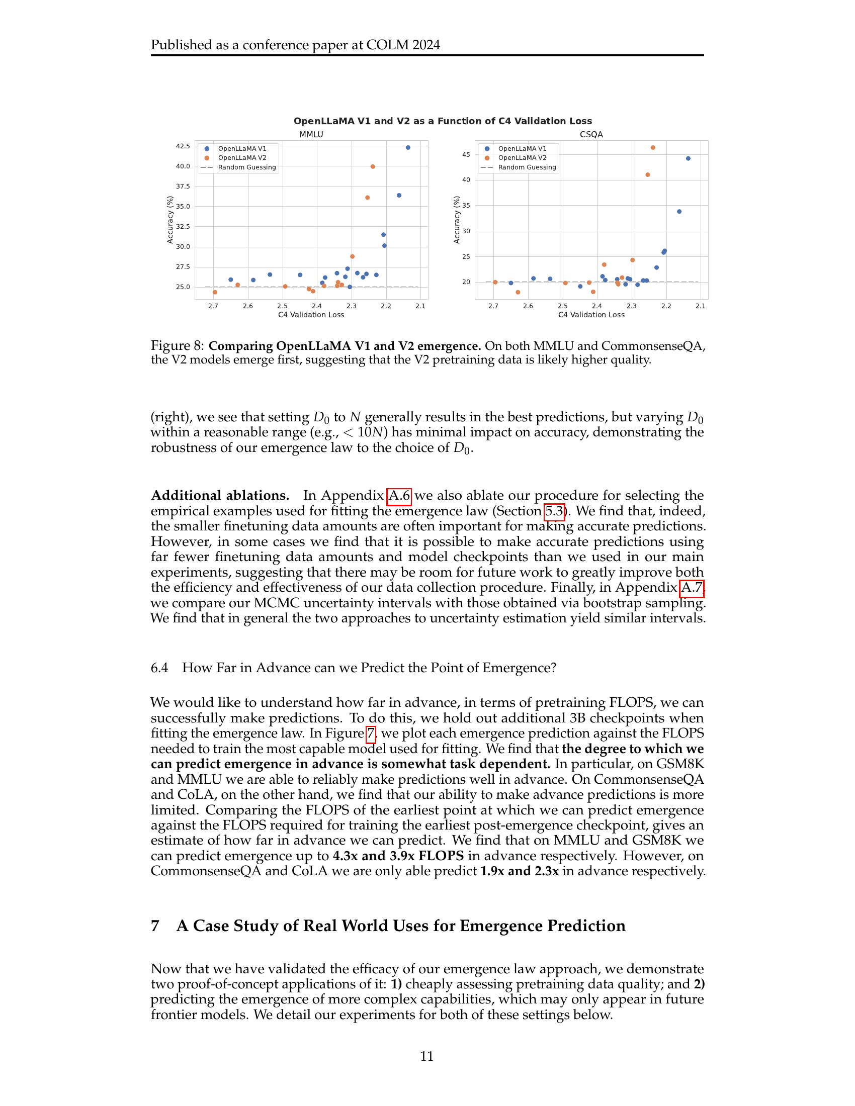
🔼 Figure 8 presents a comparison of the emergence behavior of OpenLLaMA V1 and V2 language models on two benchmark tasks: MMLU and CommonsenseQA. Emergence refers to the point at which a model’s performance on a task suddenly surpasses random chance. The x-axis represents the C4 validation loss, a measure of the model’s performance during pretraining. The y-axis shows the model’s accuracy on the respective benchmark task. The plot demonstrates that for both MMLU and CommonsenseQA, the OpenLLaMA V2 models achieve emergence at a lower C4 validation loss than the V1 models. This suggests that the pretraining data used for OpenLLaMA V2 is of higher quality, leading to the faster emergence of capabilities in the model. The difference in emergence point highlights the impact of pretraining data quality on model performance.
read the caption
Figure 8: Comparing OpenLLaMA V1 and V2 emergence. On both MMLU and CommonsenseQA, the V2 models emerge first, suggesting that the V2 pretraining data is likely higher quality.

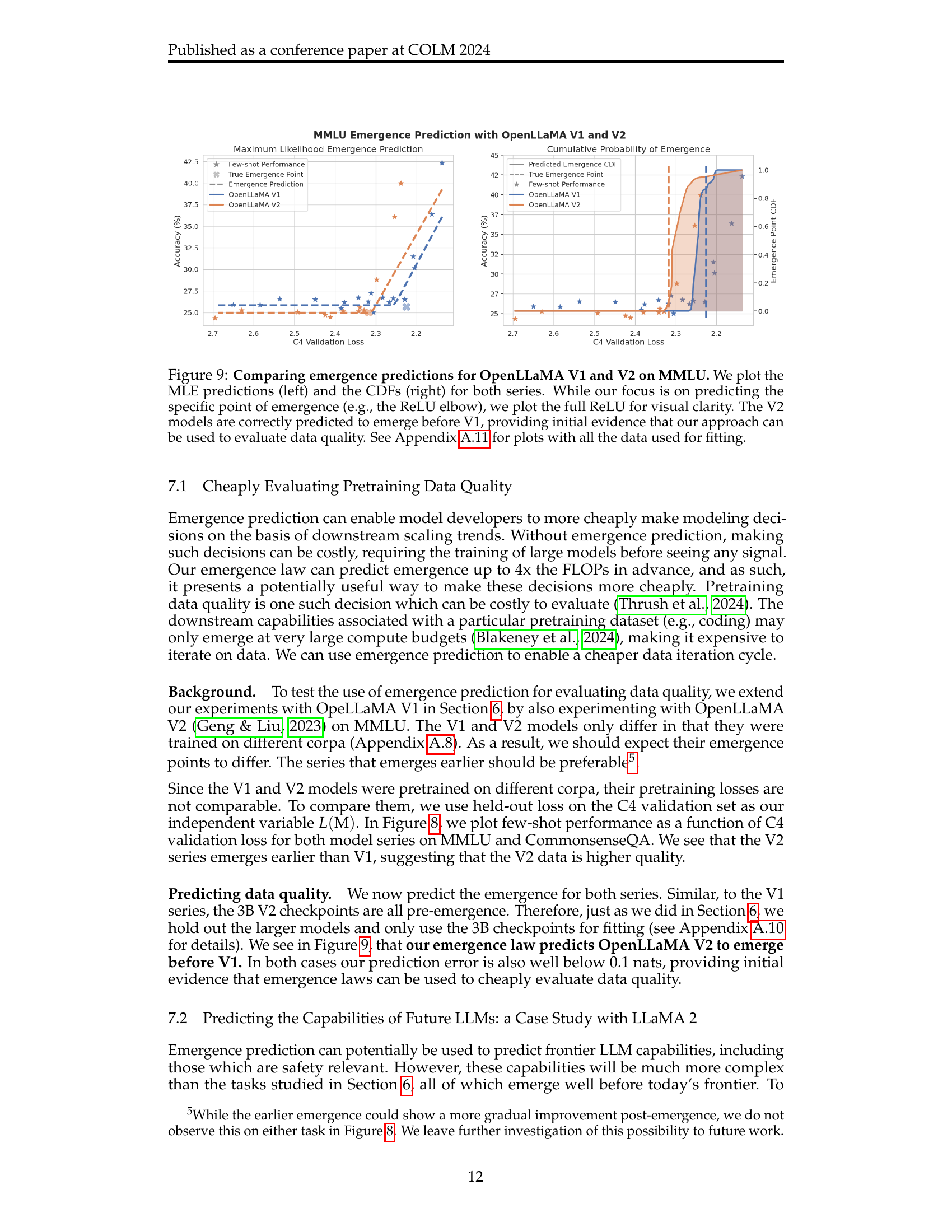
🔼 Figure 9 presents a comparison of emergence predictions for two versions of the OpenLLaMA language model (V1 and V2) when evaluated on the MMLU benchmark. The left panel shows maximum likelihood estimates (MLE) of the emergence point (the model scale at which capabilities suddenly improve) for each model version. The right panel displays cumulative distribution functions (CDFs) of the emergence point, illustrating the probability distribution for where emergence might occur. A key observation is that the model trained on the V2 data is predicted to demonstrate emergence at a smaller model scale than V1, aligning with the expectation based on the improved pretraining data quality indicated in the paper. Appendix A.11 provides additional visualizations.
read the caption
Figure 9: Comparing emergence predictions for OpenLLaMA V1 and V2 on MMLU. We plot the MLE predictions (left) and the CDFs (right) for both series. While our focus is on predicting the specific point of emergence (e.g., the ReLU elbow), we plot the full ReLU for visual clarity. The V2 models are correctly predicted to emerge before V1, providing initial evidence that our approach can be used to evaluate data quality. See Appendix A.11 for plots with all the data used for fitting.

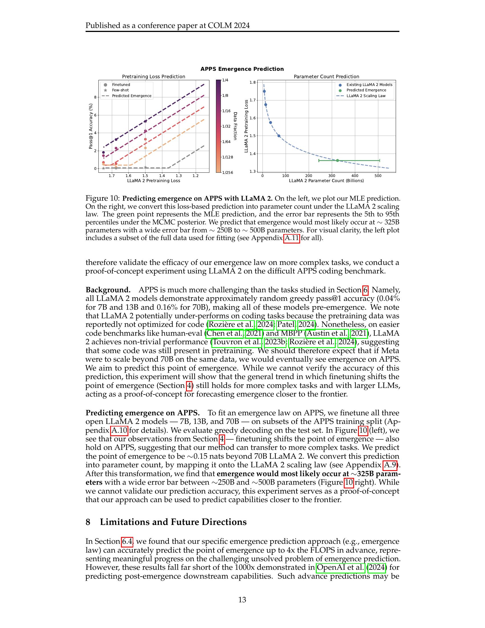
🔼 Figure 10 presents the findings on predicting the emergence of capabilities in LLaMA 2 models on the APPS benchmark. The left panel displays the maximum likelihood estimation (MLE) of the emergence point, represented as a function of pretraining loss. The right panel converts this loss-based prediction into a parameter count, leveraging the LLaMA 2 scaling law. The green point indicates the MLE prediction, with the error bar showing the 5th to 95th percentiles derived from Markov Chain Monte Carlo (MCMC) posterior sampling. This analysis predicts that emergence is most likely to occur around 325 billion parameters, but with substantial uncertainty ranging from 250B to 500B parameters.
read the caption
Figure 10: Predicting emergence on APPS with LLaMA 2. On the left, we plot our MLE prediction. On the right, we convert this loss-based prediction into parameter count under the LLaMA 2 scaling law. The green point represents the MLE prediction, and the error bar represents the 5th to 95th percentiles under the MCMC posterior. We predict that emergence would most likely occur at ∼325similar-toabsent325\sim 325∼ 325B parameters with a wide error bar from ∼250similar-toabsent250\sim 250∼ 250B to ∼500similar-toabsent500\sim 500∼ 500B parameters. For visual clarity, the left plot includes a subset of the full data used for fitting (see Appendix A.11 for all).

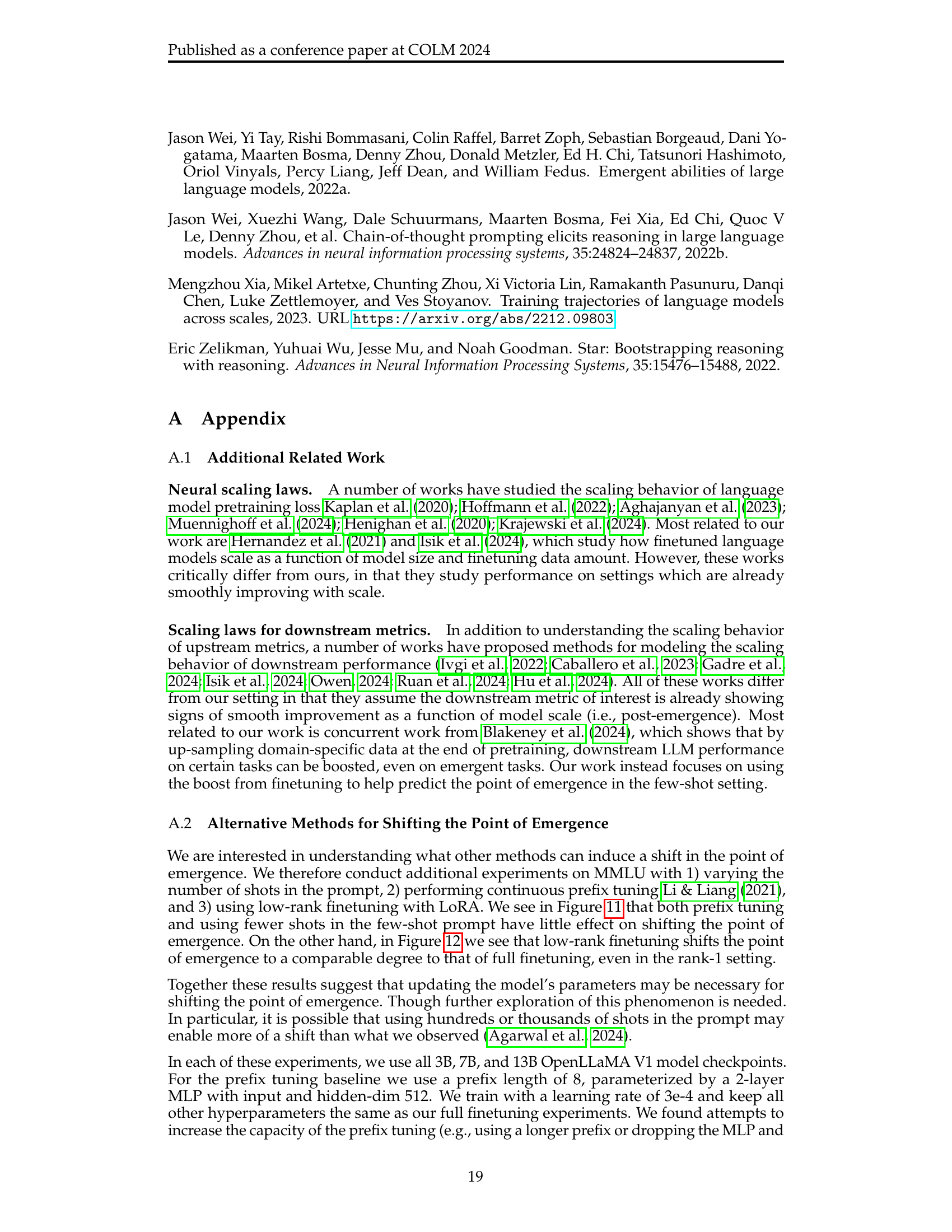
🔼 This figure shows the results of two experiments to determine whether prefix tuning or the number of shots used affects the point at which capabilities emerge in language models. The left panel shows that while prefix tuning improves performance after emergence, it does not shift the point at which capabilities emerge. The right panel shows that using zero-shot prompting instead of five-shot prompting also does not shift the emergence point. This suggests that techniques like prefix tuning and altering the number of shots are not effective at changing when capabilities emerge.
read the caption
Figure 11: One the left we compare full fine-tuning against continuous prefix tuning on MMLU. We find that prefix tuning provides effectively no shift to the point of emergence, despite improving the performance of post-emergence models. On the right we compare 0-shot verses 5-shot prompting on MMLU. We see that using fewer shots has no meaningful effect on the point of emergence. Together these results suggest that the ability for prompt tuning to shift the point of emergence is very limited.

🔼 This figure compares the impact of different LoRA ranks (1, 2, 4, 64) and full finetuning on the emergence of capabilities in a language model. It shows how varying the rank affects the point at which the model begins to perform non-randomly (emergence point) on the MMLU benchmark. The key finding is that even low-rank LoRA finetuning (rank 1) significantly shifts this emergence point, almost as much as full finetuning. This demonstrates the effectiveness of LoRA in rapidly achieving substantial performance gains, even in the context of emergent capabilities.
read the caption
Figure 12: Comparing LoRA finetuning, with rank 1, 2, 4, and 64 against full finetuning on MMLU. We see that LoRA finetuning even with rank 1 shifts the point of emergence to a comparable degree to that of full finetuning.

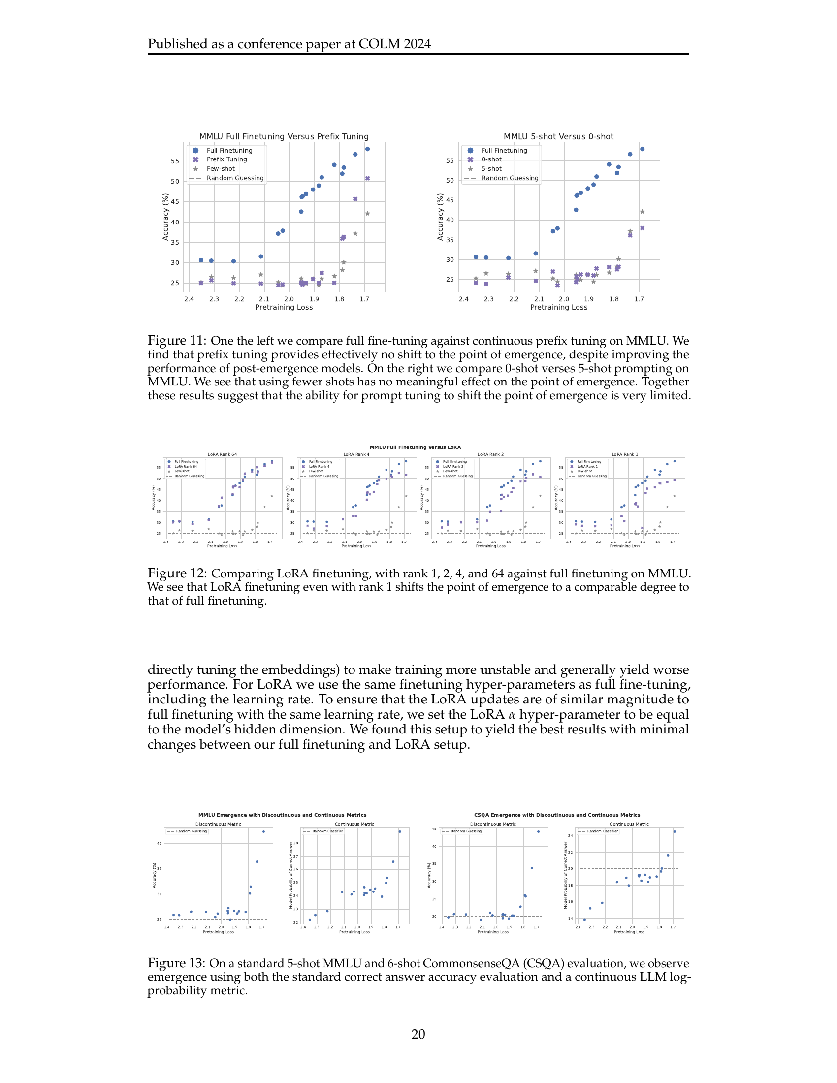
🔼 This figure demonstrates that the phenomenon of emergence in large language models is not solely an artifact of using discontinuous metrics. It shows that even when evaluating model performance using a continuous metric (LLM log-probability), rather than a discrete metric (accuracy), the characteristic ’emergent’ behavior—a sudden improvement beyond random chance—is still observed. Two standard benchmarks, MMLU (5-shot) and CommonsenseQA (6-shot), are used for this demonstration.
read the caption
Figure 13: On a standard 5-shot MMLU and 6-shot CommonsenseQA (CSQA) evaluation, we observe emergence using both the standard correct answer accuracy evaluation and a continuous LLM log-probability metric.

🔼 Figure 14 presents a detailed analysis of how model size affects both the emergence point and post-emergence performance scaling in large language models (LLMs). The emergence point, where performance significantly improves beyond random chance, and the scaling of performance after emergence are plotted against the pretraining loss for four standard NLP benchmarks (MMLU, GSM8K, CommonsenseQA, and CoLA). Data is shown for three model sizes (3B, 7B, and 13B parameters) using both few-shot and finetuned settings. The key finding is the consistent relationship between pretraining loss and performance across all model sizes and settings, indicating that pretraining loss is a reliable indicator of LLM capabilities.
read the caption
Figure 14: We plot few-shot and full data finetuning performance as a function of pretraining loss using all 3B, 7B, and 13B model checkpoints for all tasks. We see that both the point of emergence and the downstream performance scaling thereafter, as a function of pretraining loss, is consistent across model size in both the few-shot and finetuned setting.

🔼 Figure 15 shows the scaling law fit for the LLaMA 2 series of models. The x-axis represents the parameter count (in billions), and the y-axis shows the pretraining loss. The plot displays the data points for the different LLaMA 2 models (7B, 13B, 34B, and 70B parameters) along with the fitted scaling law curve. The equation of the fitted curve is also provided, showing the relationship between the parameter count (N) and pretraining loss (L(N)). The figure demonstrates that the pretraining loss of LLaMA 2 models closely follows the predicted scaling law, indicating a good fit.
read the caption
Figure 15: We plot our scaling law fit for the LLaMA 2 series of models. We also include the learned values for our final fit on the plot. In this case N𝑁Nitalic_N corresponds to parameter count in billions. We see that the LLaMA 2 models are well modeled by our scaling law.

🔼 Figure 16 shows the maximum likelihood predictions of the emergence point for four NLP tasks (GSM8K, MMLU, CSQA, CoLA) using the proposed emergence law. The figure displays the model’s fit across different amounts of finetuning data (shown in multiple colors) for each task. A gray line represents the model’s extrapolated prediction for the emergence point in the few-shot setting. The results demonstrate the accuracy of the emergence law in predicting the point where a model exhibits a sudden improvement beyond random chance performance, typically within a margin of 0.1 nats and often significantly smaller.
read the caption
Figure 16: We plot the maximum likelihood predictions from our emergence law on each task. These plots include results from every finetuning run used for fitting the emergence law. The grey line represents our extrapolated prediction and the multi-color lines correspond to the fit produced by the emergence law for the various data levels. We see that across all tasks we are able to successfully predict the point of emergence within 0.1 nats and in many cases much less than that.

🔼 This figure compares the emergence predictions for OpenLLaMA V1 and V2 language models on the MMLU benchmark. The x-axis represents the C4 validation loss, a measure of the model’s performance on a general language understanding task. The y-axis shows the accuracy on the MMLU benchmark. Multiple colored lines show the performance of models fine-tuned with varying amounts of data, demonstrating how the point of emergence shifts depending on the amount of training data. A grey line represents an extrapolated prediction of the emergence point using a fitted emergence law. The results show that the emergence point for both V1 and V2 models can be predicted with high accuracy (within 0.1 nats). This suggests that the methodology can effectively anticipate when a model will demonstrate emergent capabilities.
read the caption
Figure 17: We plot the maximum likelihood predictions from our emergence law with OpenLLaMA V1 (left) and OpenLLaMA V2 (right) on MMLU. We plot C4 Validation loss on the x-axis. These plots include results from every finetuning run used for fitting the emergence law. The grey line represents our extrapolated prediction and the multi-color lines correspond to the fit produced by the emergence law for the various data levels. We see that in both cases we are able to successfully predict the point of emergence within 0.1 nats.

🔼 Figure 18 displays the results of applying an emergence prediction model to the APPS benchmark using LLaMA 2. The left panel shows the maximum likelihood estimate of emergence (grey line) alongside model fits using different amounts of training data (colored lines). The right panel shows the cumulative distribution function (CDF) of the emergence point’s posterior distribution, indicating confidence and uncertainty in the prediction. The model predicts that emergence will likely occur at a pretraining loss roughly 0.15 nats beyond the LLaMA 2 70B parameter model.
read the caption
Figure 18: We plot the MLE prediction (left) and MCMC CDF (right) for our emergence law fit using LLaMA 2 on APPS. The left plot includes results from every finetuning run used for fitting the emergence law. The grey line represents our extrapolated prediction and the multi-color lines correspond to the fit produced by the emergence law for the various data levels. We see that our emergence law predicts emergence roughly 0.15 nats beyond the LLaMA 2 70B model.

🔼 This figure displays the cumulative distribution function (CDF) of the model’s predicted emergence point for four different NLP tasks (GSM8K, MMLU, CSQA, and CoLA). The x-axis represents the model’s pretraining loss, while the y-axis shows the cumulative probability of emergence. Each CDF curve shows a sharp increase near the actual emergence point (marked by a star), indicating high confidence in the prediction near the actual emergence point. However, the CDFs also have a moderately long tail extending beyond the emergence point, demonstrating some uncertainty in precisely predicting the point at which the capabilities emerge, especially when the model displays low performance before exhibiting emergent behavior. The stars represent the actual few-shot performance data, illustrating the pre-emergence phase’s near-random accuracy and subsequent sharp improvement after the emergence threshold.
read the caption
Figure 19: We plot the cumulative distribution function of our estimated posterior distribution over the point of emergence on each task. The stars correspond to few-shot performance on the task and represent the true emergence curve. The point at which the slope of the CDF peaks represents the mode of the distribution. We see across all tasks that the distribution spikes near the true point of emergence and is followed by a moderately long tail.
More on tables
| Ablation Setting | GSM8K | MMLU | CSQA | CoLA |
|---|---|---|---|---|
| Full Data | 0.022 [0.004, 0.170] | 0.041 [0.011, 0.055] | 0.003 [0.001, 0.045] | 0.064 [0.030, 0.121] |
| -1 Smallest Subset | 0.014 [0.002, 0.051] | 0.022 [0.010, 0.031] | 0.051 [0.037, 0.084] | 0.071 [0.024, 0.097] |
| -2 Smallest Subset | 0.047 [0.018, 0.063] | 0.025 [0.003, 0.032] | 0.087 [0.063, 0.129] | 0.634 [0.577, 0.711] |
| -3 Smallest Subset | 0.005 [0.002, 0.050] | 0.001 [0.002, 0.025] | 0.988 [0.913, 1.099] | 1.513 [1.291, 1.698] |
| -1 Largest Subset | 0.022 [0.002, 0.032] | 0.034 [0.024, 0.034] | 0.045 [0.003, 0.096] | 0.036 [0.007, 0.090] |
| -2 Largest Subset | 0.005 [0.002, 0.054] | 1.017 [1.482, 1.985] | 0.057 [0.056, 0.059] | 0.004 [0.002, 0.058] |
| -3 Largest Subset | 0.016 [0.002, 0.083] | 0.332 [1.371, 4.200] | 0.089 [0.077, 0.098] | 0.044 [0.019, 0.143] |
| Only Subset Sample 1 | 0.006 [0.001, 0.031] | 0.244 [0.223, 0.489] | 1.557 [1.616, 2.573] | 0.179 [0.125, 0.269] |
| Only Subset Sample 2 | 0.026 [0.002, 0.067] | 0.073 [0.059, 0.077] | 0.035 [0.004, 0.102] | 0.034 [0.022, 0.047] |
| Last 6 Checkpoints | 0.010 [0.003, 0.113] | 0.041 [0.007, 0.049] | 0.075 [0.063, 0.301] | 0.118 [0.087, 0.167] |
| Last 5 Checkpoints | 0.047 [0.048, 0.176] | 0.032 [0.020, 0.038] | 1.165 [1.070, 1.728] | 0.130 [0.099, 0.170] |
| Last 4 Checkpoints | 0.080 [0.072, 4.925] | 0.030 [0.001, 0.042] | 1.734 [1.555, 2.308] | 0.076 [0.052, 0.111] |
| Last 3 Checkpoints | 0.159 [0.124, 0.703] | 0.013 [0.002, 0.059] | 0.986 [0.802, 1.249] | 0.039 [0.004, 0.077] |
| Last 6 Checkpoints, Every Other Even | 0.019 [0.003, 0.162] | 0.070 [0.059, 0.075] | 1.663 [1.667, 1.781] | 0.033 [0.007, 0.050] |
| Last 6 Checkpoints, Every Other Odd | 0.044 [0.041, 0.126] | 0.040 [0.024, 0.045] | 0.037 [0.031, 0.191] | 0.224 [0.190, 0.287] |
| -1 Last Checkpoints | 0.069 [0.003, 0.149] | 0.043 [0.023, 0.055] | 0.985 [0.858, 1.800] | 0.026 [0.004, 0.079] |
| -2 Last Checkpoints | 0.087 [0.003, 0.176] | 0.076 [0.046, 0.089] | 0.102 [0.098, 0.104] | 0.165 [0.098, 0.242] |
| -3 Last Checkpoints | 0.110 [0.010, 0.468] | 0.664 [0.500, 0.959] | 0.616 [0.510, 0.822] | 2.217 [2.031, 2.407] |
| -4 Last Checkpoints | 0.044 [0.005, 0.089] | 2.308 [2.347, 57.068] | 0.581 [0.546, 1.169] | 1.039 [0.905, 1.298] |
🔼 This table presents the results of ablations conducted on the emergence prediction method. The main goal is to assess the impact of using different subsets of finetuning data and varying numbers of model checkpoints when fitting the emergence law. The table shows the absolute error between the predicted and actual emergence points, along with 5th and 95th percentile errors from MCMC sampling. Errors larger than 0.1 nats are marked in red (indicating failure). The top row shows the baseline using all data, the middle rows show results with various amounts of held-out finetuning data to analyze data selection’s impact, and the bottom rows vary the number of model checkpoints used for fitting to determine the minimum number needed for accurate predictions. More details on the ablations are in Appendix A.6.
read the caption
Table 2: Ablating the effect of holding out different finetuning subsets and model checkpoints when fitting the emergence law. We present the absolute error between the maximum likelihood predicted point of emergence and the ground-truth. In brackets we include the 5th and 95th percentile of prediction errors produced by our MCMC posterior sampling. We consider fits where the maximum likelihood prediction is greater than 0.1 nats from the ground-truth to be failures and highlight these cases in red; otherwise we highlight in green. In the top row we present results for the fit obtained using all finetuning data amounts and model checkpoints. In the middle rows (e.g., “-1 Smallest Subset” to “Only Subset Sample 2”), we present ablations in which we hold out various finetuning data subsets, so as to understand the effect of our data subset selection methodology on our predictions. Finally, in the bottom rows, we present ablations in which we hold out various model checkpoints, so as to understand how many checkpoints are needed to obtain good predictions (e.g., “Last 6 Checkpoints” to “-4 Last Checkpoint”). We describe each ablation in more detail in Appendix A.6.
| Task | Method | 5% | 10% | 25% | 50% | 75% | 90% | 95% | MLE | GT |
|---|---|---|---|---|---|---|---|---|---|---|
| GSM8K | MCMC | 1.813 | 1.852 | 1.900 | 1.937 | 1.970 | 1.992 | 2.003 | 2.006 | 1.984 |
| Bootstrap | 1.978 | 1.984 | 1.995 | 2.007 | 2.021 | 2.031 | 2.036 | |||
| MMLU | MCMC | 1.825 | 1.828 | 1.837 | 1.847 | 1.858 | 1.866 | 1.869 | 1.855 | 1.814 |
| Bootstrap | 1.818 | 1.825 | 1.836 | 1.848 | 1.859 | 1.867 | 1.871 | |||
| CSQA | MCMC | 1.781 | 1.810 | 1.821 | 1.829 | 1.835 | 1.840 | 1.843 | 1.830 | 1.827 |
| Bootstrap | 1.723 | 1.736 | 1.815 | 1.835 | 1.846 | 1.857 | 1.863 | |||
| CoLA | MCMC | 1.712 | 1.724 | 1.742 | 1.761 | 1.779 | 1.795 | 1.804 | 1.769 | 1.833 |
| Bootstrap | 1.738 | 1.746 | 1.758 | 1.770 | 1.782 | 1.791 | 1.798 | |||
| MMLU C4 V1 | MCMC | 2.207 | 2.221 | 2.241 | 2.246 | 2.255 | 2.259 | 2.261 | 2.254 | 2.226 |
| Bootstrap | 2.183 | 2.200 | 2.216 | 2.228 | 2.238 | 2.246 | 2.250 | |||
| MMLU C4 V2 | MCMC | 2.264 | 2.275 | 2.289 | 2.306 | 2.310 | 2.316 | 2.320 | 2.311 | 2.318 |
| Bootstrap | 2.249 | 2.257 | 2.272 | 2.284 | 2.296 | 2.305 | 2.311 | |||
| APPS | MCMC | 1.324 | 1.332 | 1.344 | 1.357 | 1.370 | 1.380 | 1.386 | 1.361 | — |
| Bootstrap | 1.285 | 1.304 | 1.330 | 1.352 | 1.370 | 1.385 | 1.393 |
🔼 This table compares two methods for estimating the uncertainty of emergence predictions: Markov Chain Monte Carlo (MCMC) and bootstrapping. For each task (MMLU, GSM8K, CSQA, CoLA, and APPS), it shows the 5th, 10th, 25th, 50th, 75th, 90th, and 95th percentiles of the emergence point’s pretraining loss, as determined by each method. The maximum likelihood estimate (MLE) and the ground truth are also provided for comparison. The results demonstrate that both methods generally produce similar uncertainty estimates. The table is organized into three sections: the first shows results for the tasks in Section 6.2, the second shows results for the data quality experiments in Section 7.1, and the third presents the results for the APPS experiment in Section 7.2. The ‘MMLU C4 V1’ and ‘MMLU C4 V2’ rows refer to the OpenLLaMA model versions used.
read the caption
Table 3: Comparing emergence prediction uncertainty estimates obtained via MCMC and bootstrapping. On each task, we present seven a range of percentiles for the point of emergence in terms of pretraining loss for each distribution. We also present the maximum likelihood prediction (“MLE”), and the ground-truth (“GT”) point of emergence. We see that both methods generally produce similar distributions. In the top section we present the uncertainties for each task used in Section 6.2. In the middle we include uncertainties for the data quality experiments in Section 7.1. “MMLU C4 V1” refers to the OpenLLaMA V1 fit and “MMLU C4 V2” refers to the V2 fit. At the bottom, we include uncertainties for the APPS experiment in Section 7.2.
Full paper#
