↗ arXiv ↗ Hugging Face ↗ Papers with Code
TL;DR#
Self-supervised learning (SSL) for 3D data is hampered by the scarcity and cost of acquiring real-world 3D datasets. This necessitates the development of methods for utilizing easily obtainable data, such as synthetic data. Current SSL methods, however, struggle to learn meaningful representations from procedurally generated shapes that lack semantic information. Existing 3D datasets have limitations in scalability, availability, and copyright restrictions.
This paper introduces Point-MAE-Zero, a novel approach that leverages procedural 3D programs to automatically generate a large-scale synthetic dataset. This dataset is then used to pre-train a Point-MAE model (Point-MAE-Zero), which surprisingly achieves comparable or even better performance on downstream 3D tasks such as object classification, part segmentation, and masked point cloud completion compared to models trained on human-annotated datasets like ShapeNet. The results indicate that current self-supervised learning methods primarily focus on geometric features rather than semantic information, and they open up opportunities for using more abundant synthetic data in 3D representation learning.
Key Takeaways#
Why does it matter?#
This paper is crucial because it tackles the data scarcity challenge in 3D representation learning. By demonstrating that high-quality representations can be learned from synthetic data generated by procedural 3D programs, it opens new avenues for research and development in various 3D applications, reducing reliance on expensive and limited real-world datasets. It also challenges the assumptions in existing SSL methods by showing that geometric structures, rather than high-level semantics, are primarily captured.
Visual Insights#

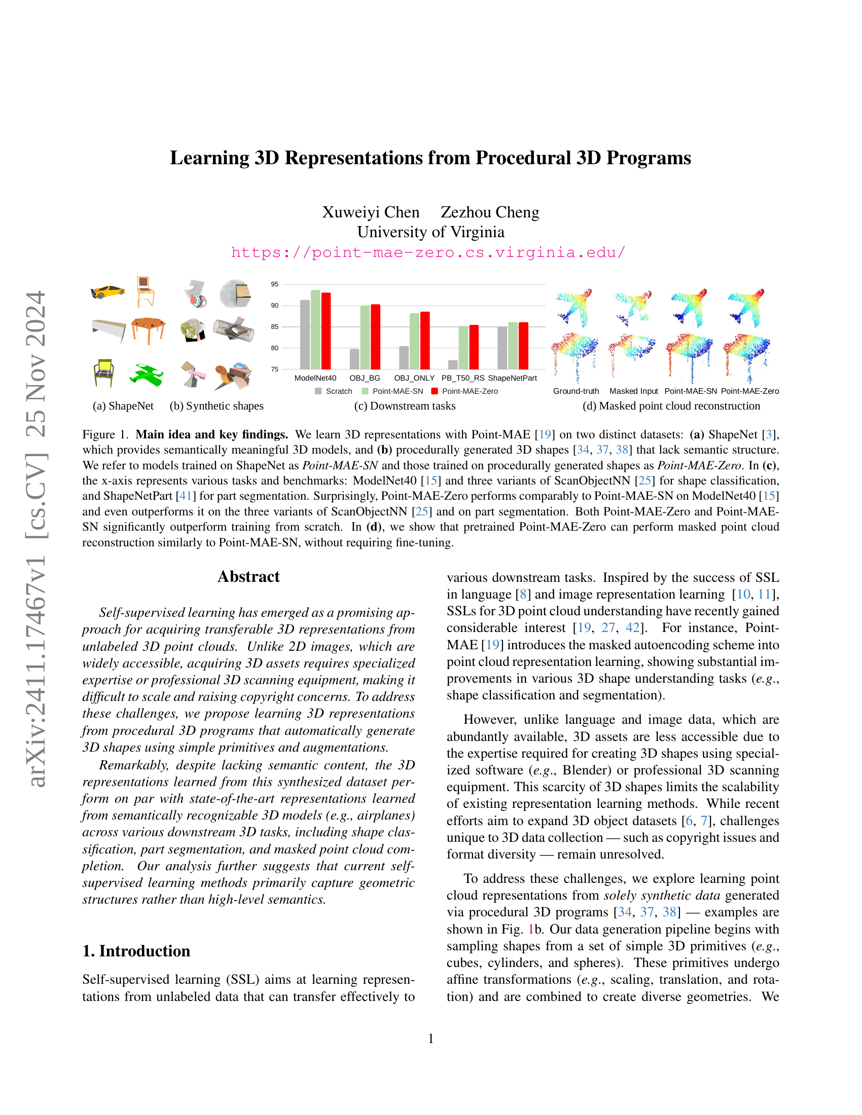
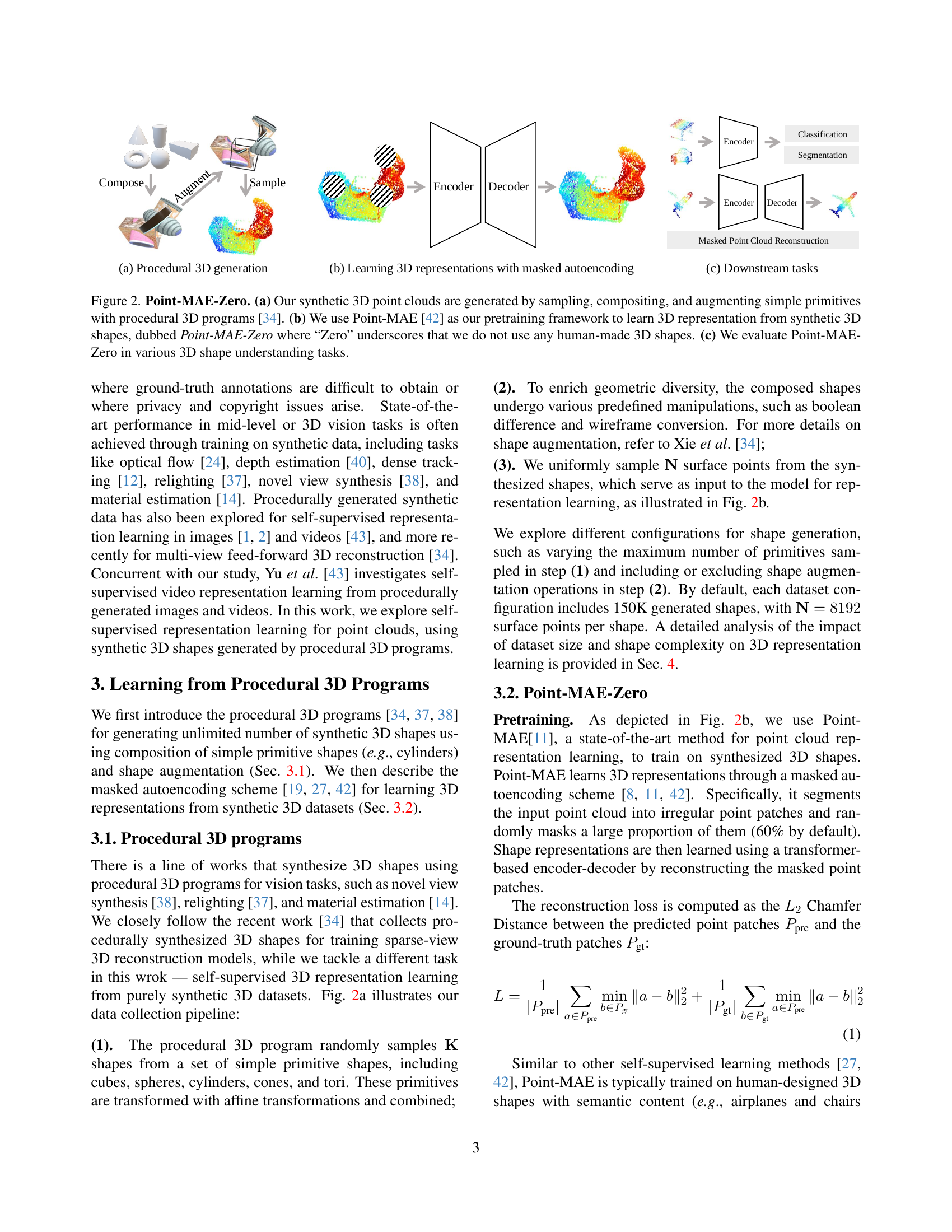
🔼 Figure 1 illustrates the Point-MAE-Zero framework. (a) shows the process of generating synthetic 3D point clouds using procedural programs: simple primitives are sampled, combined, and augmented. (b) details the self-supervised learning approach where Point-MAE is used to learn 3D representations from these synthetic shapes, a model referred to as Point-MAE-Zero (the ‘Zero’ indicates no use of human-created 3D data). (c) shows the downstream tasks used to evaluate the effectiveness of the learned representations.
read the caption
Figure 1: Point-MAE-Zero. (a) Our synthetic 3D point clouds are generated by sampling, compositing, and augmenting simple primitives with procedural 3D programs [34]. (b) We use Point-MAE [42] as our pretraining framework to learn 3D representation from synthetic 3D shapes, dubbed Point-MAE-Zero where “Zero” underscores that we do not use any human-made 3D shapes. (c) We evaluate Point-MAE-Zero in various 3D shape understanding tasks.
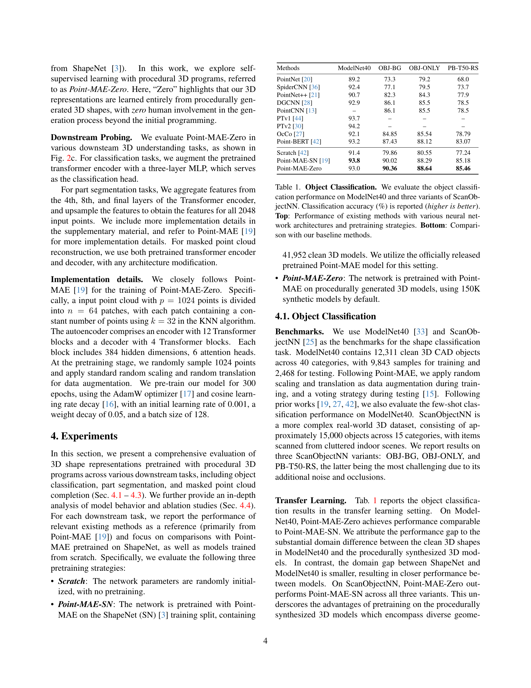
| Methods | ModelNet40 | OBJ-BG | OBJ-ONLY | PB-T50-RS |
|---|---|---|---|---|
| PointNet [20] | 89.2 | 73.3 | 79.2 | 68.0 |
| SpiderCNN [36] | 92.4 | 77.1 | 79.5 | 73.7 |
| PointNet++ [21] | 90.7 | 82.3 | 84.3 | 77.9 |
| DGCNN [28] | 92.9 | 86.1 | 85.5 | 78.5 |
| PointCNN [13] | – | 86.1 | 85.5 | 78.5 |
| PTv1 [44] | 93.7 | – | – | – |
| PTv2 [30] | 94.2 | – | – | – |
| OcCo [27] | 92.1 | 84.85 | 85.54 | 78.79 |
| Point-BERT [42] | 93.2 | 87.43 | 88.12 | 83.07 |
| Scratch [42] | 91.4 | 79.86 | 80.55 | 77.24 |
| Point-MAE-SN [19] | 93.8 | 90.02 | 88.29 | 85.18 |
| Point-MAE-Zero | 93.0 | 90.36 | 88.64 | 85.46 |
🔼 This table presents a comparison of object classification accuracy across different methods on the ModelNet40 benchmark dataset and three variations of ScanObjectNN. It shows the performance of various state-of-the-art methods, highlighting the neural network architecture and pre-training strategies used. The bottom section contrasts these existing methods against the performance of the models presented in the paper (Point-MAE-SN and Point-MAE-Zero). Higher accuracy percentages indicate better performance.
read the caption
Table 1: Object Classification. We evaluate the object classification performance on ModelNet40 and three variants of ScanObjectNN. Classification accuracy (%) is reported (higher is better). Top: Performance of existing methods with various neural network architectures and pretraining strategies. Bottom: Comparison with our baseline methods.
In-depth insights#
Procedural 3D SSL#
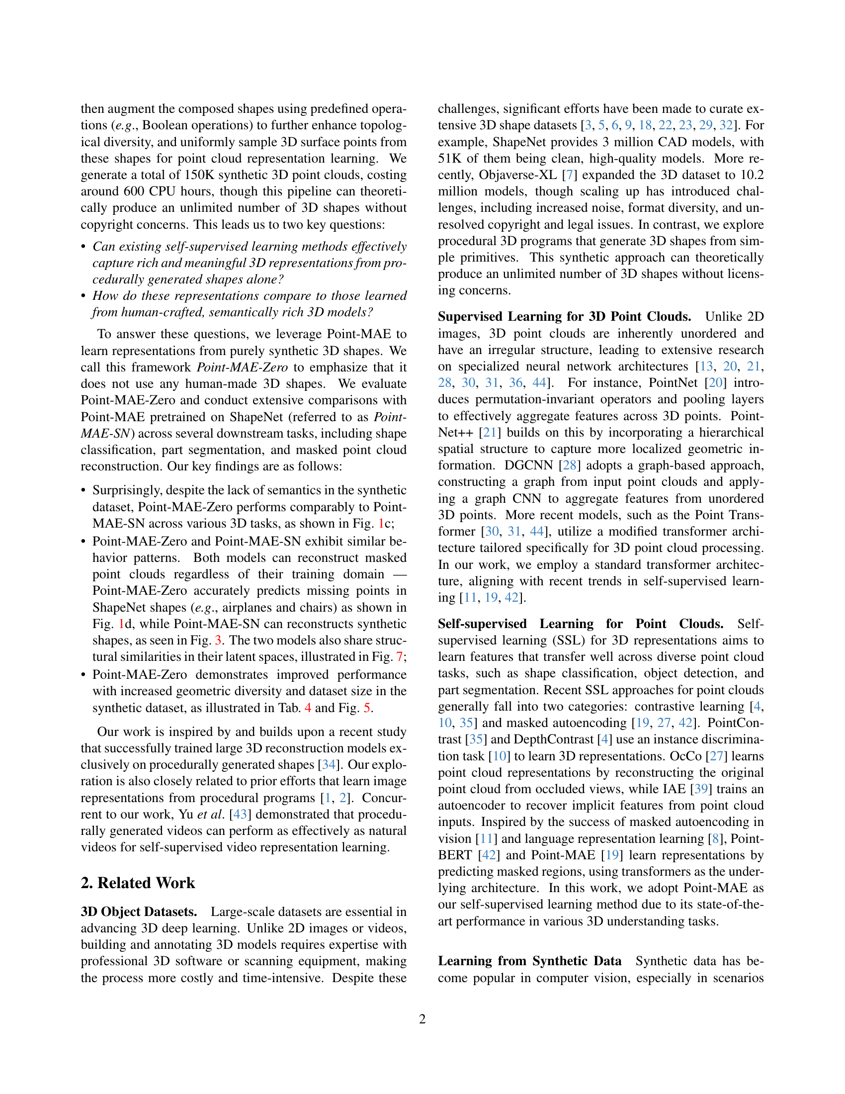
Procedural 3D self-supervised learning (SSL) represents a significant advancement in 3D representation learning. By leveraging procedurally generated synthetic data, this approach overcomes limitations associated with the scarcity and cost of real-world 3D datasets, while simultaneously addressing copyright concerns. The core idea is to train a model on a large number of diverse shapes automatically created using simple primitives and augmentations, effectively learning geometric structures without relying on semantic labels. This strategy is particularly valuable because it allows for scalable training and the generation of unlimited data, making the approach highly cost-effective and easily reproducible. Remarkably, models trained on this synthetic data demonstrate comparable or even superior performance to those trained on established datasets containing semantically meaningful data on downstream tasks such as shape classification and part segmentation. This highlights the potential for procedural 3D SSL to become a dominant paradigm in 3D representation learning, enabling broader access to high-quality 3D models and facilitating significant advances in various 3D understanding tasks. Further research should explore the limitations and potential biases of purely synthetic data, and investigate the balance between geometric and semantic information learned through different self-supervised approaches.
Point-MAE Zero#
The proposed “Point-MAE Zero” methodology presents a novel approach to self-supervised 3D representation learning. It leverages procedurally generated synthetic 3D shapes, bypassing the limitations and costs associated with acquiring real-world 3D datasets. This synthetic data generation pipeline is efficient and avoids copyright issues, offering scalability. Remarkably, despite the lack of semantic information in the procedurally generated data, Point-MAE Zero achieves performance on par with models trained on semantically rich datasets like ShapeNet, suggesting that geometric structures are the primary features captured by self-supervised learning methods. This highlights the importance of geometric diversity in training data for effective 3D representation learning and opens up possibilities for using similar approaches in other domains where obtaining labeled data is expensive or challenging. The success of Point-MAE Zero underscores the potential of synthetic data generation for advancing 3D deep learning research.
Synth Data Transfer#
The concept of ‘Synth Data Transfer’ in the context of 3D representation learning is intriguing. It speaks to the ability of models trained on synthetically generated data to effectively transfer their learned representations to real-world tasks. The success of this transfer is critically dependent on the quality and diversity of the synthetic dataset. If the synthetic data accurately reflects the statistical properties and geometric complexities of real-world 3D shapes, then the model should generalize well. However, a crucial challenge lies in bridging the semantic gap: synthetic data often lacks the rich semantic information present in real-world scans. Therefore, the focus should be on generating diverse and realistic synthetic datasets that capture geometric and topological features effectively. Moreover, careful evaluation is vital to quantify how well the learned features transfer and identify any limitations or biases introduced by the synthetic data. This evaluation should consider various downstream tasks and benchmarks to provide a holistic assessment of the transferability.
Geometric Focus#
A hypothetical “Geometric Focus” section in a 3D representation learning paper would delve into the model’s inherent bias towards geometric properties over semantic understanding. The core argument would likely center on the observation that self-supervised models, trained on both procedurally generated and semantically rich datasets, demonstrate comparable performance on downstream tasks. This suggests that the learned representations primarily capture geometric structures, such as symmetry and topology, rather than high-level semantic information (e.g., object categories). The analysis might include visualizations of feature spaces, showing similar clustering patterns across datasets despite the semantic differences. Ablation studies, varying the complexity and diversity of the training data, would further support this geometric focus, demonstrating that increasing geometric complexity improves performance regardless of semantic content. The findings would challenge the assumption that high-level semantic understanding is crucial for effective 3D representation learning, indicating that geometric structure plays a dominant role. Furthermore, the discussion may propose future research to bridge the gap between geometry and semantics, suggesting methods to incorporate semantic information in self-supervised training to potentially enhance performance further.
Future of 3D SSL#
The future of 3D self-supervised learning (SSL) is bright, driven by the need for efficient and scalable methods to learn from vast, unlabeled 3D data. Procedural generation of synthetic data offers a promising avenue, providing virtually unlimited, copyright-free assets for training. However, challenges remain. Bridging the gap between synthetic and real-world data is crucial; current methods struggle to seamlessly generalize from synthetic domains to real-world scenarios. Future research should focus on developing more sophisticated data augmentation techniques to simulate the complexities of real-world 3D data. Moreover, exploring alternative self-supervised learning paradigms beyond masked autoencoding, such as contrastive learning or generative models, could unlock greater representational power. Improving efficiency and scalability are also paramount. Training large 3D models on massive datasets is computationally expensive; developing more efficient training algorithms and architectures is essential to make 3D SSL more accessible. Finally, developing better evaluation metrics that capture the nuances of 3D representation learning is vital for objectively assessing progress in the field. The development of new benchmarks and metrics tailored specifically to the complexities of 3D data will be essential to guide future research and encourage the creation of more robust and reliable 3D SSL models.
More visual insights#
More on figures

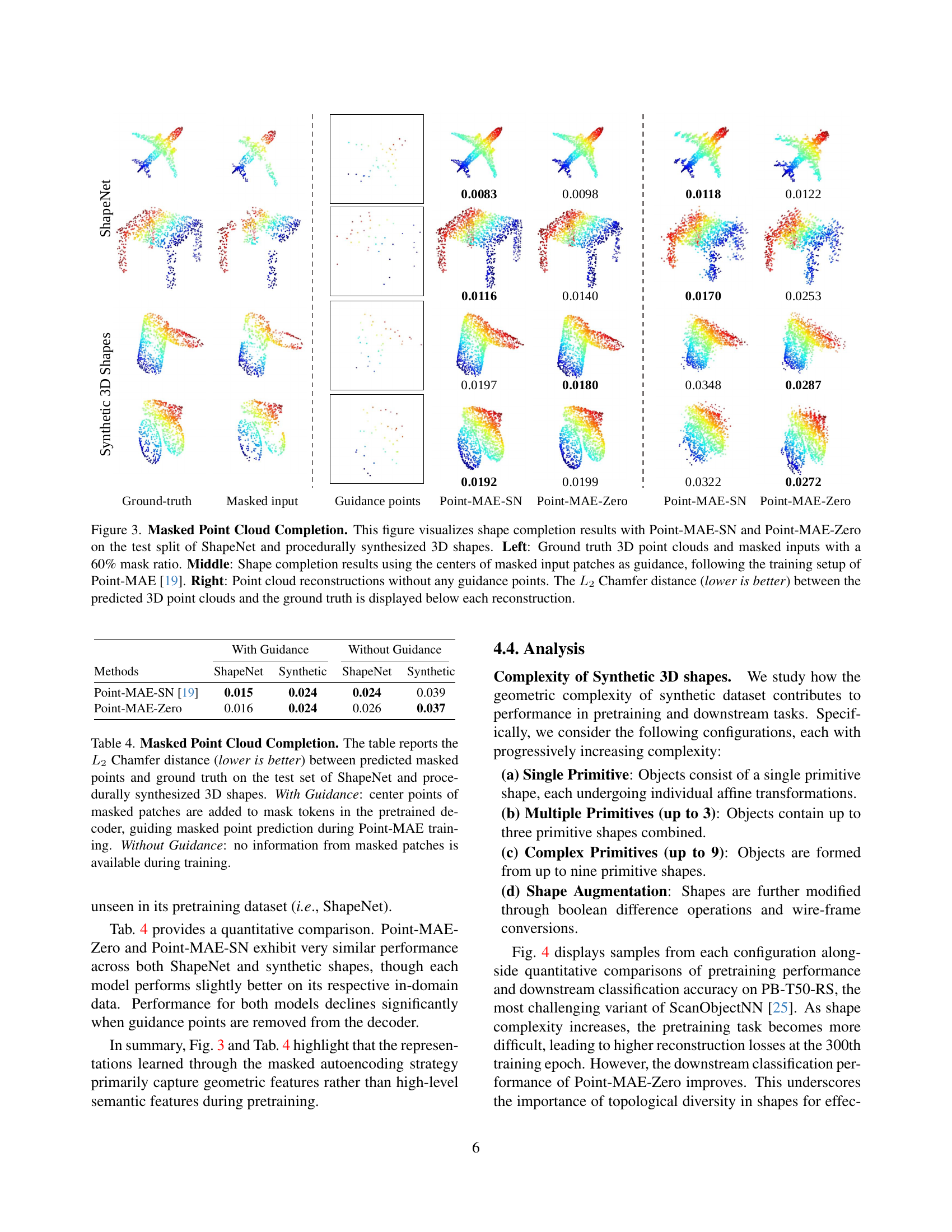
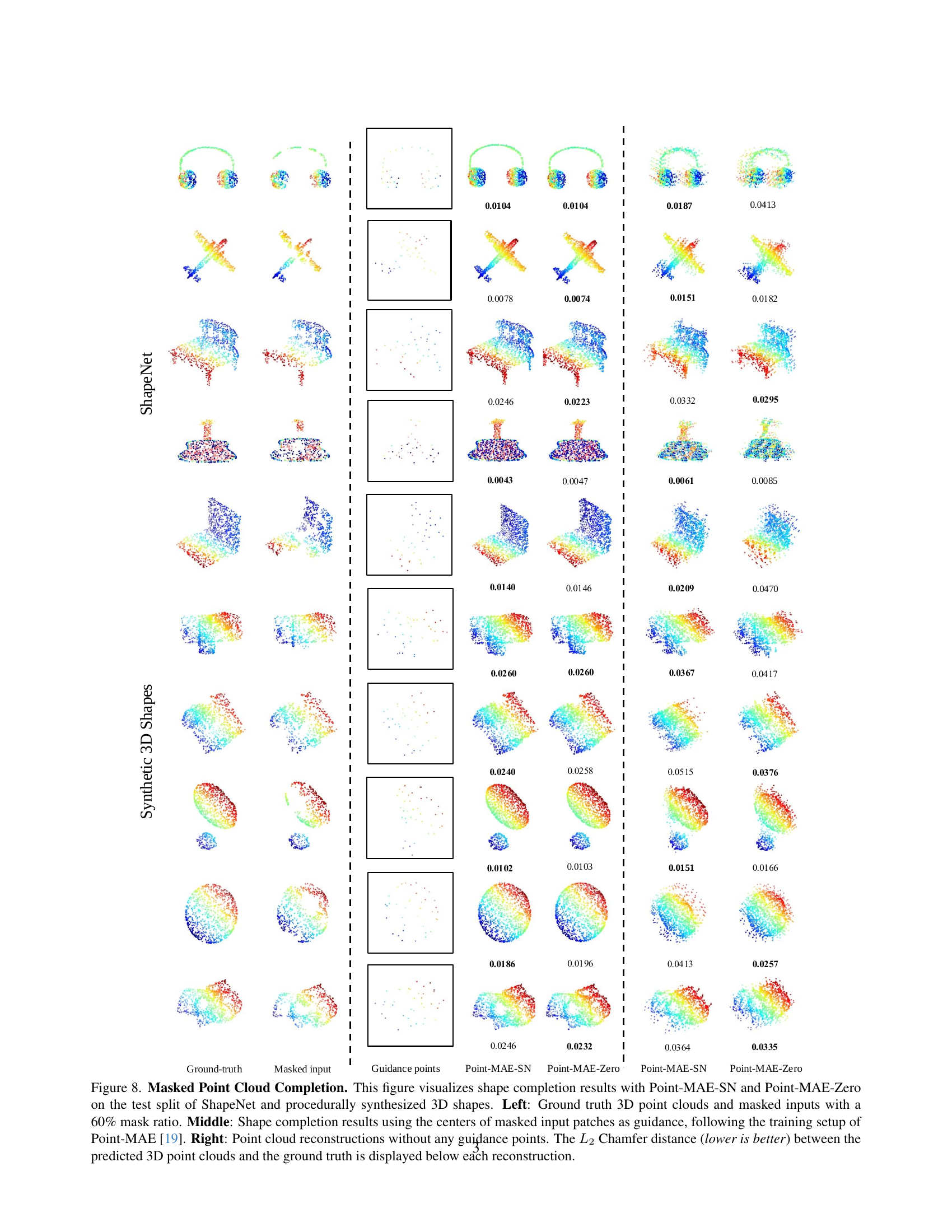
🔼 Figure 2 demonstrates the performance of Point-MAE-SN and Point-MAE-Zero models on masked point cloud completion. It uses ShapeNet and procedurally generated 3D shapes. The left column shows the ground truth point clouds and masked versions (60% masked). The middle column shows reconstruction results using guidance points (centers of masked patches), mirroring the Point-MAE training methodology. The right column displays reconstruction results without using any guidance points. The Chamfer distance, a metric measuring the difference between the reconstructed and ground truth point clouds, is shown beneath each reconstruction.
read the caption
Figure 2: Masked Point Cloud Completion. This figure visualizes shape completion results with Point-MAE-SN and Point-MAE-Zero on the test split of ShapeNet and procedurally synthesized 3D shapes. Left: Ground truth 3D point clouds and masked inputs with a 60% mask ratio. Middle: Shape completion results using the centers of masked input patches as guidance, following the training setup of Point-MAE [19]. Right: Point cloud reconstructions without any guidance points. The L2subscript𝐿2L_{2}italic_L start_POSTSUBSCRIPT 2 end_POSTSUBSCRIPT Chamfer distance (lower is better) between the predicted 3D point clouds and the ground truth is displayed below each reconstruction.

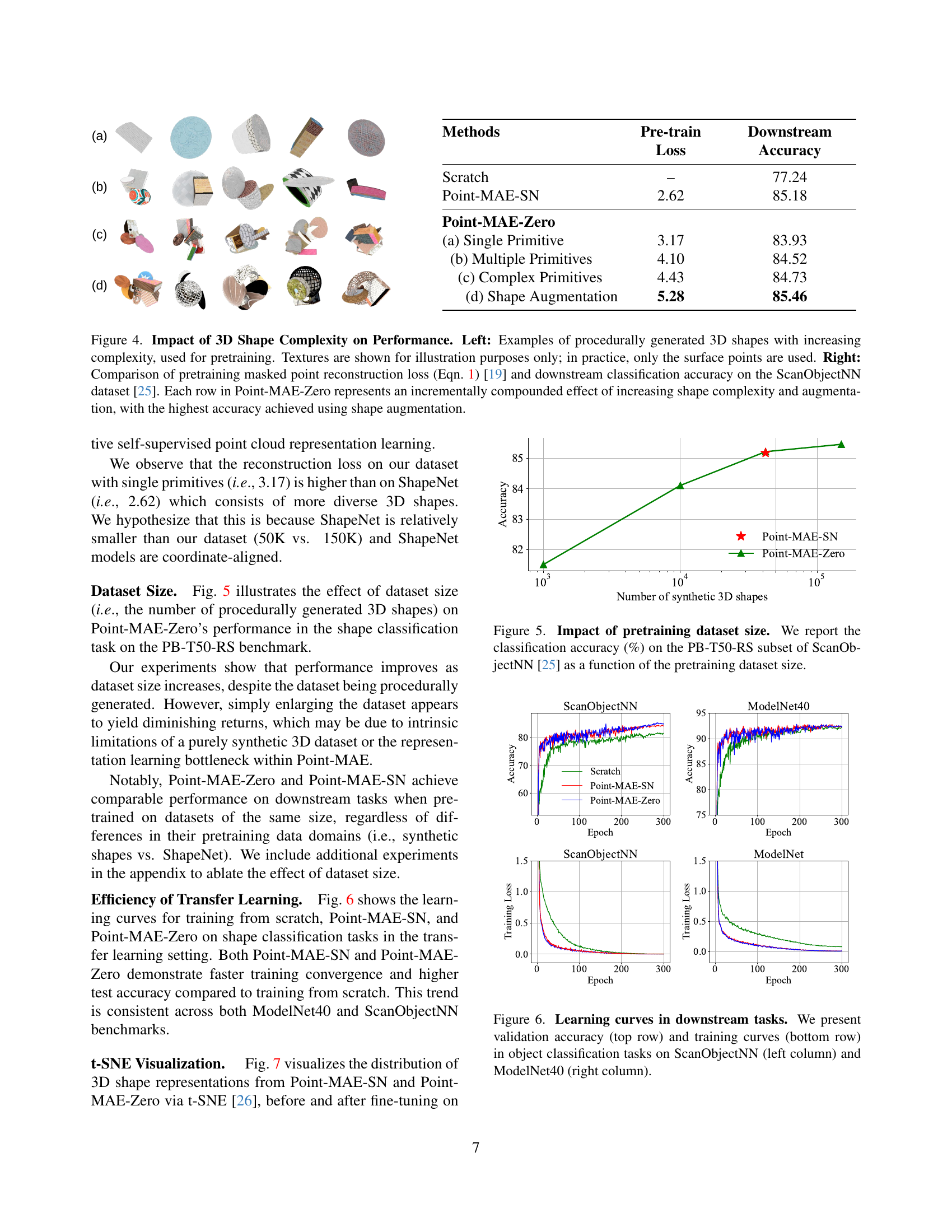
🔼 Figure 3 demonstrates how increasing the complexity of procedurally generated 3D shapes used for pretraining affects model performance. The left panel shows examples of shapes, starting with simple primitives and progressing to more complex shapes created through combinations and augmentations. The right panel presents a quantitative comparison, showing that while increasing complexity initially increases the pretraining loss (masked point cloud reconstruction loss, as defined in Equation 1 of the referenced Point-MAE paper), it ultimately leads to higher downstream classification accuracy on the ScanObjectNN dataset. Each row in the ‘Point-MAE-Zero’ section represents a step-wise increase in shape complexity and the application of augmentations, culminating in the highest accuracy when augmentations are included.
read the caption
Figure 3: Impact of 3D Shape Complexity on Performance. Left: Examples of procedurally generated 3D shapes with increasing complexity, used for pretraining. Textures are shown for illustration purposes only; in practice, only the surface points are used. Right: Comparison of pretraining masked point reconstruction loss (Eqn. 1) [19] and downstream classification accuracy on the ScanObjectNN dataset [25]. Each row in Point-MAE-Zero represents an incrementally compounded effect of increasing shape complexity and augmentation, with the highest accuracy achieved using shape augmentation.

🔼 This figure illustrates the effect of varying the size of the training dataset on the performance of the Point-MAE-Zero model. The model’s classification accuracy on the PB-T50-RS subset of the ScanObjectNN dataset is evaluated using different numbers of synthetic 3D shapes in the pretraining dataset. The graph shows how the accuracy changes as a function of the dataset size, indicating the relationship between dataset size and model performance.
read the caption
Figure 4: Impact of pretraining dataset size. We report the classification accuracy (%) on the PB-T50-RS subset of ScanObjectNN [25] as a function of the pretraining dataset size.

🔼 This figure displays the learning curves for two object classification tasks: ScanObjectNN and ModelNet40. The top row shows the validation accuracy over training epochs, while the bottom row presents the corresponding training loss. The plots illustrate the training progress for three different methods: training from scratch, using Point-MAE pretrained on ShapeNet, and using Point-MAE pretrained on synthetic data generated by procedural 3D programs. This comparison highlights the impact of different pretraining strategies on model performance and convergence speed for both datasets.
read the caption
Figure 5: Learning curves in downstream tasks. We present validation accuracy (top row) and training curves (bottom row) in object classification tasks on ScanObjectNN (left column) and ModelNet40 (right column).

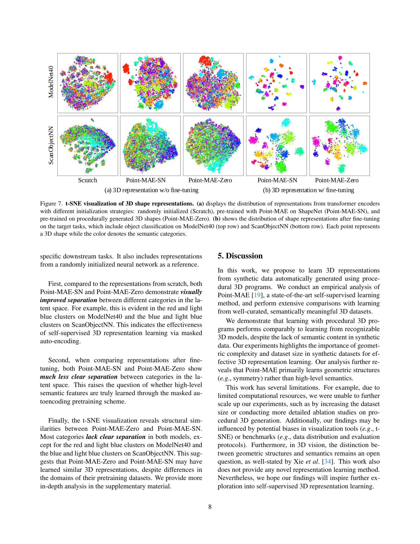
🔼 This figure visualizes the distribution of 3D shape representations learned using different methods. Panel (a) compares the representations before fine-tuning, showing the results from a randomly initialized model, a model pre-trained on ShapeNet (Point-MAE-SN), and a model pre-trained on procedurally generated 3D shapes (Point-MAE-Zero). Panel (b) shows how these representations change after fine-tuning on two object classification tasks: ModelNet40 (top) and ScanObjectNN (bottom). Each point in the t-SNE plots represents a single 3D shape, and the color of the point indicates its semantic category. This visualization helps to understand how different training methods affect the learned representations and how these representations evolve during fine-tuning.
read the caption
Figure 6: t-SNE visualization of 3D shape representations. (a) displays the distribution of representations from transformer encoders with different initialization strategies: randomly initialized (Scratch), pre-trained with Point-MAE on ShapeNet (Point-MAE-SN), and pre-trained on procedurally generated 3D shapes (Point-MAE-Zero). (b) shows the distribution of shape representations after fine-tuning on the target tasks, which include object classification on ModelNet40 (top row) and ScanObjectNN (bottom row). Each point represents a 3D shape while the color denotes the semantic categories.

🔼 Figure 7 demonstrates the performance of Point-MAE-SN and Point-MAE-Zero on masked point cloud completion. The figure shows three columns for each of several ShapeNet and synthetic 3D shapes: the ground truth complete shape; the shape with 60% of its points masked (masked input); and the completed shape generated by each model. The middle column uses the center points of masked patches as guidance during reconstruction, mirroring the Point-MAE training process. The right-most column shows reconstruction without any guidance. The L2 Chamfer distance between the generated and ground truth shapes quantifies the reconstruction error and is provided below each reconstruction.
read the caption
Figure 7: Masked Point Cloud Completion. This figure visualizes shape completion results with Point-MAE-SN and Point-MAE-Zero on the test split of ShapeNet and procedurally synthesized 3D shapes. Left: Ground truth 3D point clouds and masked inputs with a 60% mask ratio. Middle: Shape completion results using the centers of masked input patches as guidance, following the training setup of Point-MAE [19]. Right: Point cloud reconstructions without any guidance points. The L2subscript𝐿2L_{2}italic_L start_POSTSUBSCRIPT 2 end_POSTSUBSCRIPT Chamfer distance (lower is better) between the predicted 3D point clouds and the ground truth is displayed below each reconstruction.
More on tables
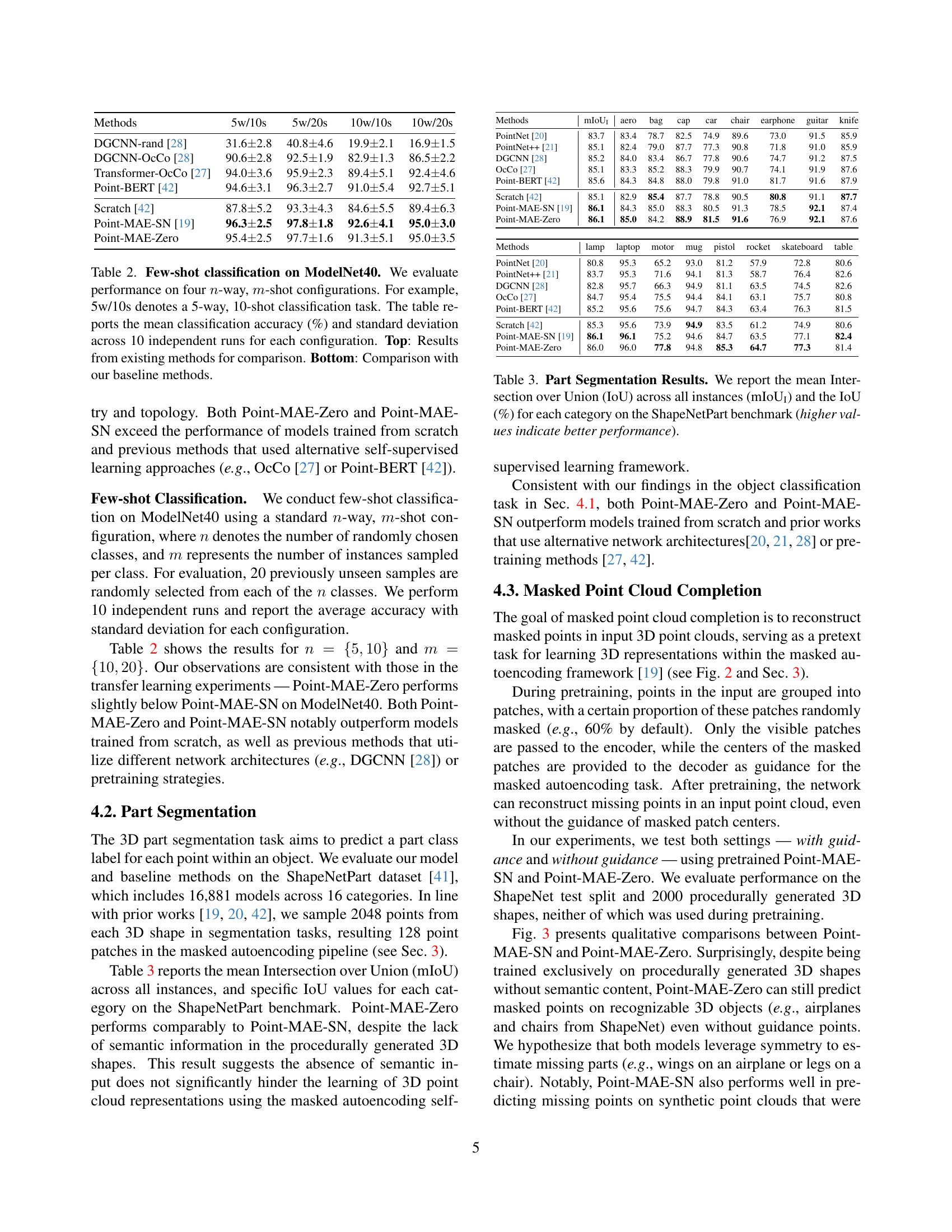
| Methods | 5w/10s | 5w/20s | 10w/10s | 10w/20s |
|---|---|---|---|---|
| DGCNN-rand [28] | 31.6 ± 2.8 | 40.8 ± 4.6 | 19.9 ± 2.1 | 16.9 ± 1.5 |
| DGCNN-OcCo [28] | 90.6 ± 2.8 | 92.5 ± 1.9 | 82.9 ± 1.3 | 86.5 ± 2.2 |
| Transformer-OcCo [27] | 94.0 ± 3.6 | 95.9 ± 2.3 | 89.4 ± 5.1 | 92.4 ± 4.6 |
| Point-BERT [42] | 94.6 ± 3.1 | 96.3 ± 2.7 | 91.0 ± 5.4 | 92.7 ± 5.1 |
| Scratch [42] | 87.8 ± 5.2 | 93.3 ± 4.3 | 84.6 ± 5.5 | 89.4 ± 6.3 |
| Point-MAE-SN [19] | 96.3 ± 2.5 | 97.8 ± 1.8 | 92.6 ± 4.1 | 95.0 ± 3.0 |
| Point-MAE-Zero | 95.4 ± 2.5 | 97.7 ± 1.6 | 91.3 ± 5.1 | 95.0 ± 3.5 |
🔼 This table presents the results of a few-shot learning experiment on the ModelNet40 dataset. Few-shot learning is a machine learning technique where a model is trained on a small number of examples for each class. The experiment evaluated the performance of different models under four different configurations, each defined by the number of classes (n-way) and the number of samples per class (m-shot). The table shows the mean classification accuracy and standard deviation across ten independent runs for each configuration. The results are compared against several existing methods and also show the performance of training the model from scratch. This allows assessment of the benefit gained through self-supervised pre-training.
read the caption
Table 2: Few-shot classification on ModelNet40. We evaluate performance on four n𝑛nitalic_n-way, m𝑚mitalic_m-shot configurations. For example, 5w/10s denotes a 5-way, 10-shot classification task. The table reports the mean classification accuracy (%) and standard deviation across 10 independent runs for each configuration. Top: Results from existing methods for comparison. Bottom: Comparison with our baseline methods.
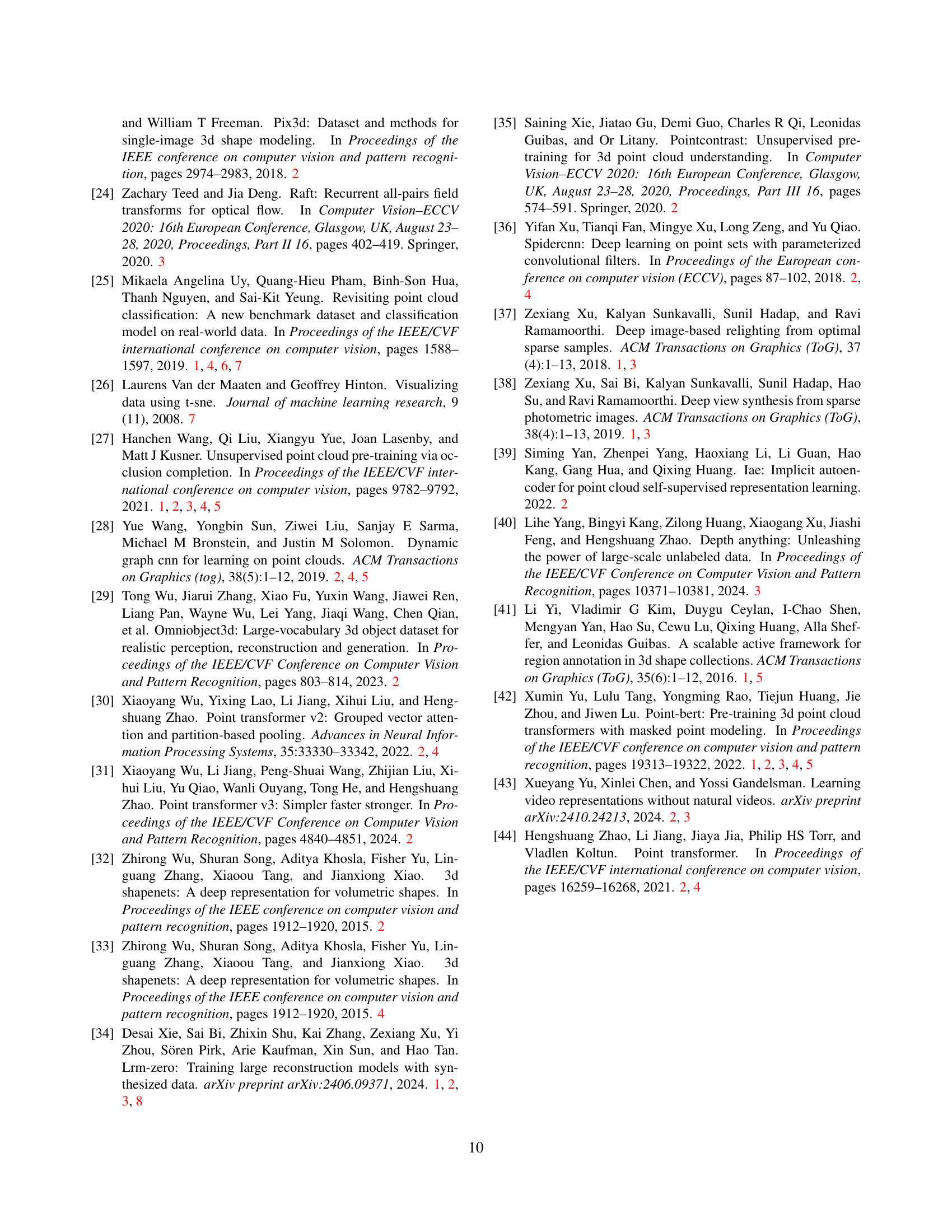
| Methods | mIoUI | aero | bag | cap | car | chair | earphone | guitar | knife |
|---|---|---|---|---|---|---|---|---|---|
| PointNet [20] | 83.7 | 83.4 | 78.7 | 82.5 | 74.9 | 89.6 | 73.0 | 91.5 | 85.9 |
| PointNet++ [21] | 85.1 | 82.4 | 79.0 | 87.7 | 77.3 | 90.8 | 71.8 | 91.0 | 85.9 |
| DGCNN [28] | 85.2 | 84.0 | 83.4 | 86.7 | 77.8 | 90.6 | 74.7 | 91.2 | 87.5 |
| OcCo [27] | 85.1 | 83.3 | 85.2 | 88.3 | 79.9 | 90.7 | 74.1 | 91.9 | 87.6 |
| Point-BERT [42] | 85.6 | 84.3 | 84.8 | 88.0 | 79.8 | 91.0 | 81.7 | 91.6 | 87.9 |
| Scratch [42] | 85.1 | 82.9 | 85.4 | 87.7 | 78.8 | 90.5 | 80.8 | 91.1 | 87.7 |
| Point-MAE-SN [19] | 86.1 | 84.3 | 85.0 | 88.3 | 80.5 | 91.3 | 78.5 | 92.1 | 87.4 |
| Point-MAE-Zero | 86.1 | 85.0 | 84.2 | 88.9 | 81.5 | 91.6 | 76.9 | 92.1 | 87.6 |
🔼 This table presents the results of a 3D part segmentation task. The evaluation is performed on the ShapeNetPart benchmark dataset. The key metric used is the Intersection over Union (IoU), which measures the overlap between predicted and ground truth part segmentations. The table shows the mean IoU across all instances (mIoU1) and the IoU for each individual object category in the ShapeNetPart dataset. Higher IoU values indicate better performance of the model in accurately segmenting the parts of the 3D shapes.
read the caption
Table 3: Part Segmentation Results. We report the mean Intersection over Union (IoU) across all instances (mIoUI) and the IoU (%) for each category on the ShapeNetPart benchmark (higher values indicate better performance).
| Methods | lamp | laptop | motor | mug | pistol | rocket | skateboard | table |
|---|---|---|---|---|---|---|---|---|
| PointNet [20] | 80.8 | 95.3 | 65.2 | 93.0 | 81.2 | 57.9 | 72.8 | 80.6 |
| PointNet++ [21] | 83.7 | 95.3 | 71.6 | 94.1 | 81.3 | 58.7 | 76.4 | 82.6 |
| DGCNN [28] | 82.8 | 95.7 | 66.3 | 94.9 | 81.1 | 63.5 | 74.5 | 82.6 |
| OcCo [27] | 84.7 | 95.4 | 75.5 | 94.4 | 84.1 | 63.1 | 75.7 | 80.8 |
| Point-BERT [42] | 85.2 | 95.6 | 75.6 | 94.7 | 84.3 | 63.4 | 76.3 | 81.5 |
| Scratch [42] | 85.3 | 95.6 | 73.9 | 94.9 | 83.5 | 61.2 | 74.9 | 80.6 |
| Point-MAE-SN [19] | 86.1 | 96.1 | 75.2 | 94.6 | 84.7 | 63.5 | 77.1 | 82.4 |
| Point-MAE-Zero | 86.0 | 96.0 | 77.8 | 94.8 | 85.3 | 64.7 | 77.3 | 81.4 |
🔼 Table 4 presents the L2 Chamfer distance results for masked point cloud completion. Lower values indicate better performance. The results are shown for both ShapeNet (a dataset of human-designed 3D shapes) and procedurally generated 3D shapes. Two scenarios are considered: ‘With Guidance,’ where the center points of the masked patches are used to help the model during reconstruction, and ‘Without Guidance,’ where no such information is provided. This comparison highlights the model’s ability to reconstruct masked points in different contexts.
read the caption
Table 4: Masked Point Cloud Completion. The table reports the L2subscript𝐿2L_{2}italic_L start_POSTSUBSCRIPT 2 end_POSTSUBSCRIPT Chamfer distance (lower is better) between predicted masked points and ground truth on the test set of ShapeNet and procedurally synthesized 3D shapes. With Guidance: center points of masked patches are added to mask tokens in the pretrained decoder, guiding masked point prediction during Point-MAE training. Without Guidance: no information from masked patches is available during training.
| Methods | With Guidance | Without Guidance | ||
|---|---|---|---|---|
| ShapeNet | Synthetic | ShapeNet | Synthetic | |
| Point-MAE-SN [19] | 0.015 | 0.024 | 0.024 | 0.039 |
| Point-MAE-Zero | 0.016 | 0.024 | 0.026 | 0.037 |
🔼 This table presents the results of object classification experiments using different methods. The accuracy of shape classification is evaluated on the ModelNet40 dataset and three variants of the ScanObjectNN dataset (OBJ-BG, OBJ-ONLY, and PB-T50-RS). The methods compared include training from scratch, Point-MAE pretrained on ShapeNet (Point-MAE-SN), and Point-MAE trained on procedurally generated data (Point-MAE-Zero). Higher accuracy percentages indicate better performance. The results are based on a revised evaluation setup, enhancing the rigor of the comparison. The ‘Scratch*’ row denotes the results obtained from the training from scratch baseline.
read the caption
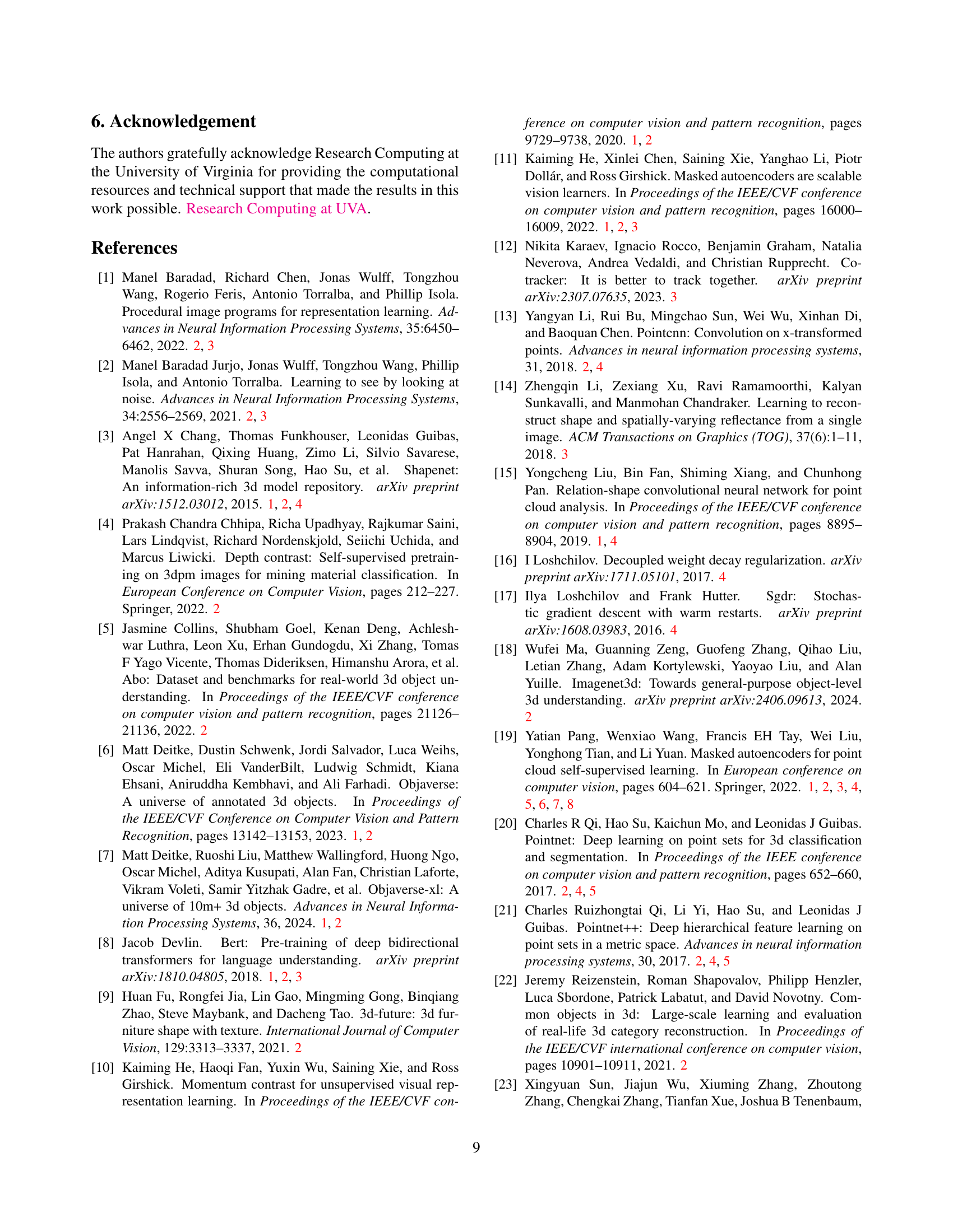
Table 5: Object Classification. Classification accuracy (%) on ModelNet40 and three ScanObjectNN variants under the revised evaluation setup (Higher is better). Note Scratch* indicates baseline method’s results we obtained.
| Methods | Pre-train Loss | Downstream Accuracy |
|---|---|---|
| Scratch | – | 77.24 |
| Point-MAE-SN | 2.62 | 85.18 |
| Point-MAE-Zero | ||
| (a) Single Primitive | 3.17 | 83.93 |
| (b) Multiple Primitives | 4.10 | 84.52 |
| (c) Complex Primitives | 4.43 | 84.73 |
| (d) Shape Augmentation | 5.28 | 85.46 |
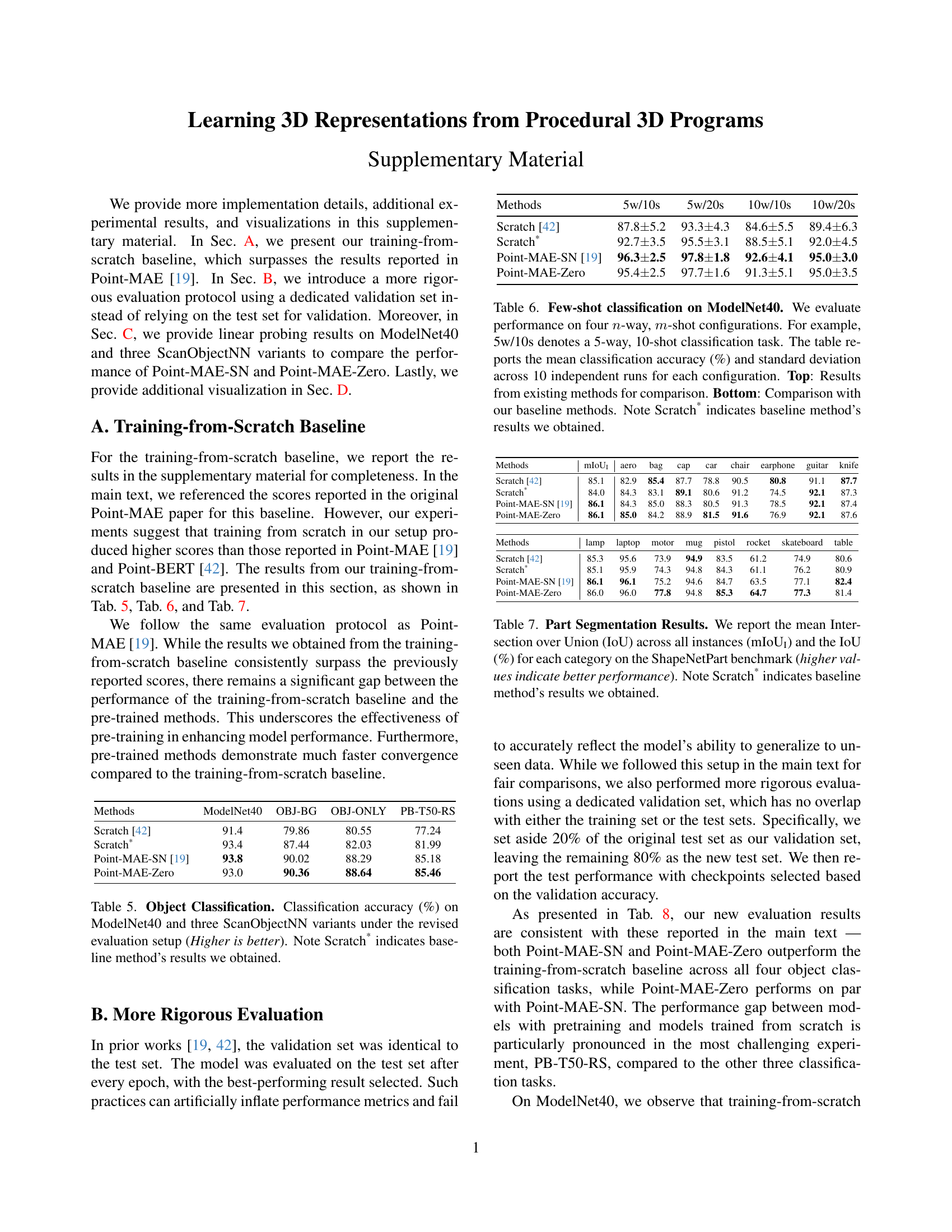
🔼 This table presents the results of a few-shot learning experiment on the ModelNet40 dataset. Few-shot learning is a machine learning technique where the model is trained on a small number of examples per class. The experiment evaluates the model’s performance under different scenarios, using different numbers of classes (n-way) and examples per class (m-shot). The table shows the mean accuracy and standard deviation across 10 independent runs for each configuration, comparing the performance of different pre-training methods (Point-MAE-SN, Point-MAE-Zero) against a baseline (Scratch*). The results highlight the effect of different pre-training strategies on few-shot learning performance.
read the caption
Table 6: Few-shot classification on ModelNet40. We evaluate performance on four n𝑛nitalic_n-way, m𝑚mitalic_m-shot configurations. For example, 5w/10s denotes a 5-way, 10-shot classification task. The table reports the mean classification accuracy (%) and standard deviation across 10 independent runs for each configuration. Top: Results from existing methods for comparison. Bottom: Comparison with our baseline methods. Note Scratch* indicates baseline method’s results we obtained.
| Methods | ModelNet40 | OBJ-BG | OBJ-ONLY | PB-T50-RS |
|---|---|---|---|---|
| Scratch [42] | 91.4 | 79.86 | 80.55 | 77.24 |
| Scratch* | 93.4 | 87.44 | 82.03 | 81.99 |
| Point-MAE-SN [19] | 93.8 | 90.02 | 88.29 | 85.18 |
| Point-MAE-Zero | 93.0 | 90.36 | 88.64 | 85.46 |
🔼 This table presents the results of 3D part segmentation on the ShapeNetPart benchmark dataset. It compares the performance of different methods, including those trained from scratch and those using pre-trained models (Point-MAE-SN and Point-MAE-Zero). The metrics used are the mean Intersection over Union (mIoU) across all instances and the IoU for each individual category. Higher values indicate better performance. A baseline result obtained from training a model from scratch is also included (indicated by Scratch*). The table allows for a comparison of the effectiveness of different approaches to 3D part segmentation.
read the caption
Table 7: Part Segmentation Results. We report the mean Intersection over Union (IoU) across all instances (mIoUI) and the IoU (%) for each category on the ShapeNetPart benchmark (higher values indicate better performance). Note Scratch* indicates baseline method’s results we obtained.
| Methods | 5w/10s | 5w/20s | 10w/10s | 10w/20s |
|---|---|---|---|---|
| Scratch [42] | 87.8 ± 5.2 | 93.3 ± 4.3 | 84.6 ± 5.5 | 89.4 ± 6.3 |
| Scratch* | 92.7 ± 3.5 | 95.5 ± 3.1 | 88.5 ± 5.1 | 92.0 ± 4.5 |
| Point-MAE-SN [19] | 96.3 ± 2.5 | 97.8 ± 1.8 | 92.6 ± 4.1 | 95.0 ± 3.0 |
| Point-MAE-Zero | 95.4 ± 2.5 | 97.7 ± 1.6 | 91.3 ± 5.1 | 95.0 ± 3.5 |
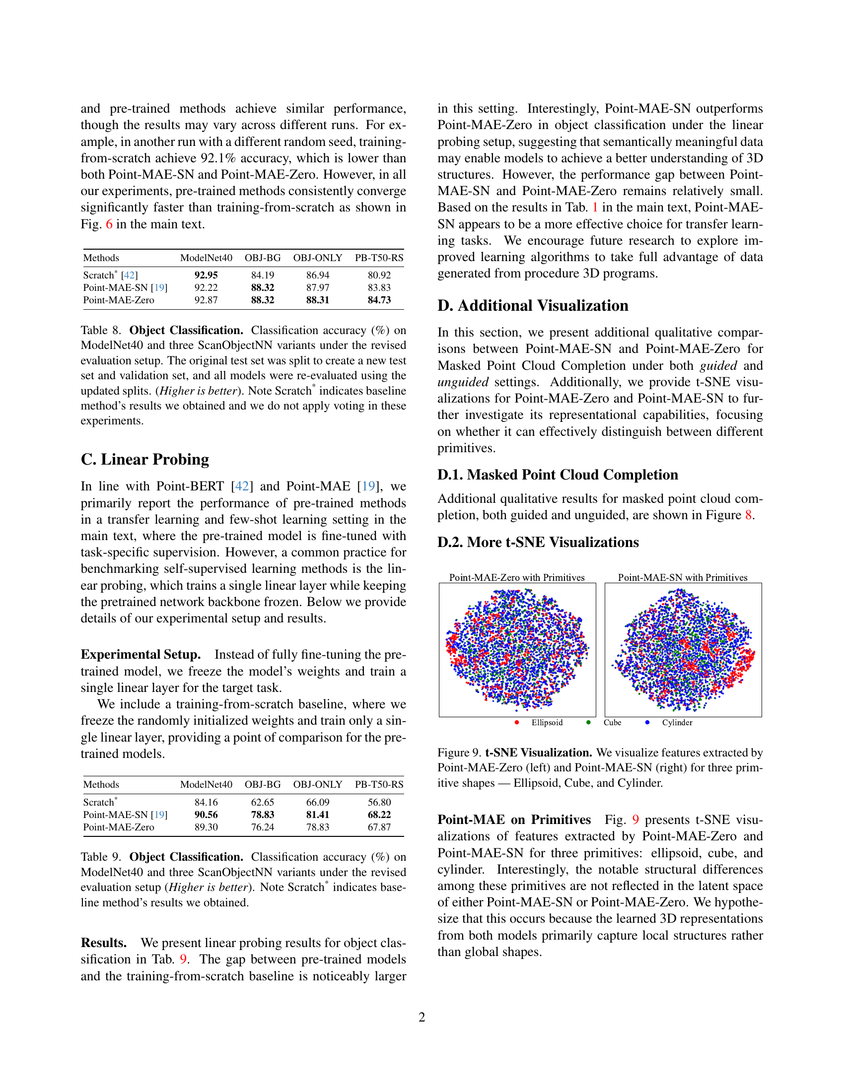
🔼 This table presents the results of object classification experiments using four different methods: a training-from-scratch baseline (Scratch*), Point-MAE pretrained on ShapeNet (Point-MAE-SN), Point-MAE-Zero, and another training-from-scratch baseline. The evaluation was performed on the ModelNet40 dataset and three variants of the ScanObjectNN dataset (OBJ-BG, OBJ-ONLY, and PB-T50-RS). To enhance the rigor of the evaluation, the original test set was divided into new test and validation sets. The reported accuracies reflect the performance of each method on the new test set, without the voting strategy used in the main paper. Higher accuracy values indicate better performance.
read the caption
Table 8: Object Classification. Classification accuracy (%) on ModelNet40 and three ScanObjectNN variants under the revised evaluation setup. The original test set was split to create a new test set and validation set, and all models were re-evaluated using the updated splits. (Higher is better). Note Scratch* indicates baseline method’s results we obtained and we do not apply voting in these experiments.
| Methods | mIoUI | aero | bag | cap | car | chair | earphone | guitar | knife |
|---|---|---|---|---|---|---|---|---|---|
| Scratch [42] | 85.1 | 82.9 | 85.4 | 87.7 | 78.8 | 90.5 | 80.8 | 91.1 | 87.7 |
| Scratch* | 84.0 | 84.3 | 83.1 | 89.1 | 80.6 | 91.2 | 74.5 | 92.1 | 87.3 |
| Point-MAE-SN [19] | 86.1 | 84.3 | 85.0 | 88.3 | 80.5 | 91.3 | 78.5 | 92.1 | 87.4 |
| Point-MAE-Zero | 86.1 | 85.0 | 84.2 | 88.9 | 81.5 | 91.6 | 76.9 | 92.1 | 87.6 |
🔼 This table presents the results of object classification using linear probing. Linear probing is a method where only a single linear layer is trained on top of a pre-trained model (Point-MAE-SN and Point-MAE-Zero), while the weights of the pre-trained model are frozen. The results are compared against a baseline of training from scratch. The evaluation was performed using a revised dataset split, different from the one reported in the main paper, to ensure more rigorous evaluation. The accuracy is measured on ModelNet40 and three variants of ScanObjectNN (OBJ-BG, OBJ-ONLY, and PB-T50-RS). Higher accuracy indicates better performance.
read the caption
Table 9: Object Classification. Classification accuracy (%) on ModelNet40 and three ScanObjectNN variants under the revised evaluation setup (Higher is better). Note Scratch* indicates baseline method’s results we obtained.
Full paper#
