↗ arXiv ↗ Hugging Face ↗ Papers with Code
TL;DR#
Multimodal Large Language Models (MLLMs) are powerful but computationally expensive. Current methods for speeding up their inference (token reduction) lack a unified approach, making comparison and improvement difficult. This paper introduces a new “filter-correlate-compress” paradigm which helps to systematically organize existing methods and improve the design of new ones.
This new paradigm has been used to create three new token reduction methods called FiCoCo. These methods significantly reduce the number of calculations needed, by as much as 82.4%, while keeping the accuracy of the results very high. This is accomplished without needing any additional training of the MLLM, making it a very practical method for accelerating inference speeds.
Key Takeaways#
Why does it matter?#
This paper is important because it addresses a critical challenge in the field of multimodal large language models (MLLMs): the high computational cost of inference. By proposing a unified paradigm for training-free token reduction and developing a suite of effective methods (FiCoCo), this research significantly accelerates MLLM inference while maintaining performance. This is crucial for making MLLMs more practical and accessible, particularly for real-world applications with resource constraints. The unified paradigm offers a valuable framework for future research in token reduction, and FiCoCo provides a set of strong baseline methods. The paper’s empirical evaluations demonstrate the practical efficacy and optimal balance between accuracy and efficiency achieved by the proposed methods.
Visual Insights#

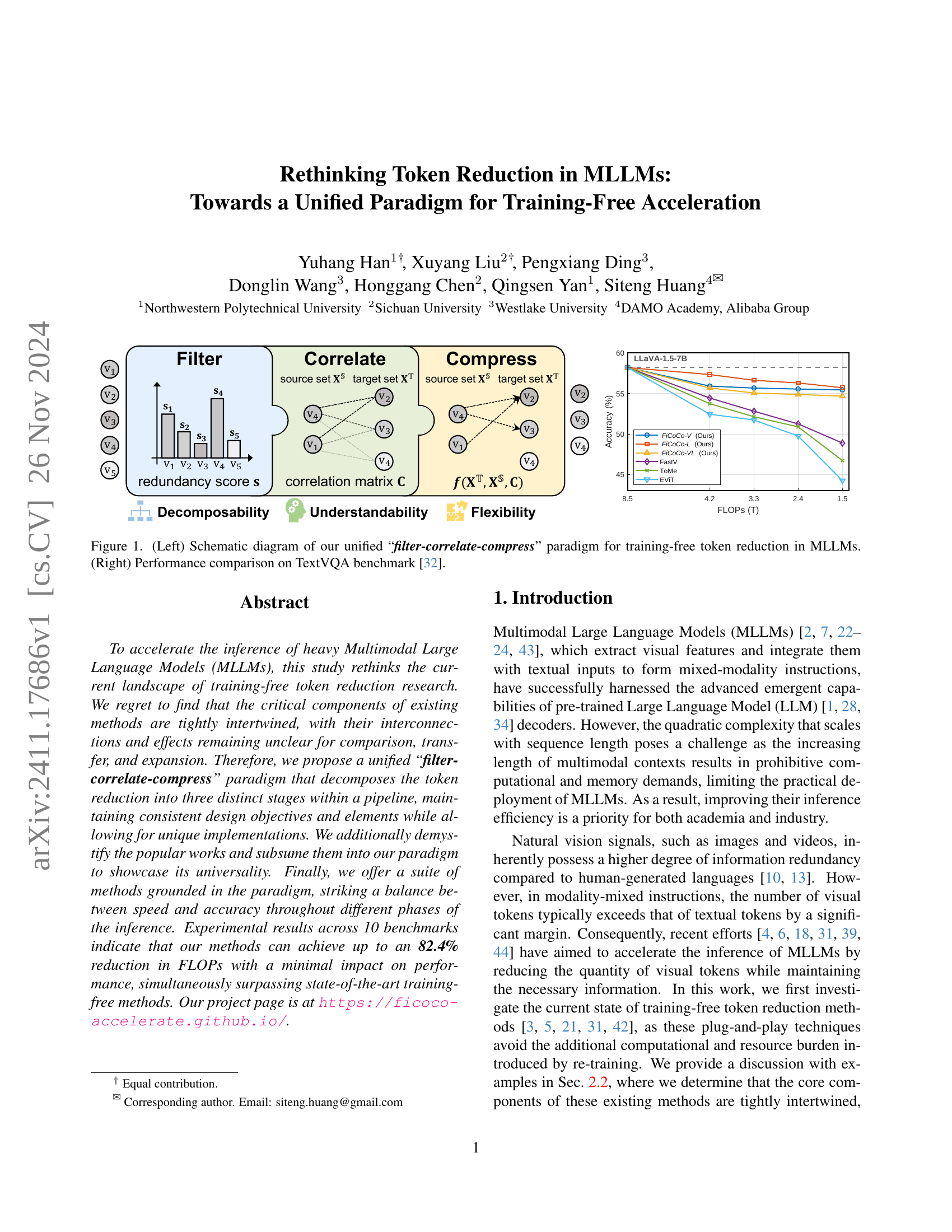
🔼 Figure 1 is a two-part illustration summarizing the core concept and experimental results of the proposed method. The left panel presents a schematic diagram outlining the unified ‘filter-correlate-compress’ paradigm. This paradigm involves three main stages: filtering redundant tokens, correlating important tokens, and finally compressing the relevant information into a reduced set of tokens, all without requiring model retraining. The right panel shows a graph comparing the performance of the proposed method (FiCoCo) to other state-of-the-art methods on the TextVQA benchmark. The graph displays accuracy as a function of FLOPs (floating-point operations), demonstrating the efficiency gains achieved by FiCoCo.
read the caption
Figure 1: (Left) Schematic diagram of our unified “filter-correlate-compress” paradigm for training-free token reduction in MLLMs. (Right) Performance comparison on TextVQA benchmark [32].
| Method | Original | Deconstructed | Δ |
|---|---|---|---|
| SQA | |||
| ToMe [3] | 65.43 | 65.42 | 0.01 |
| EViT [21] | 65.21 | 65.18 | 0.03 |
| FastV [5] | 66.98 | 66.99 | -0.01 |
| TextVQA | |||
| ToMe [3] | 52.14 | 52.14 | 0.00 |
| EViT [21] | 51.72 | 51.74 | -0.02 |
| FastV [5] | 52.83 | 52.82 | 0.01 |
🔼 This table presents a comparison of the performance of three original training-free token reduction methods (ToMe, EVIT, FastV) against their deconstructed counterparts, which are re-implemented according to the proposed ‘filter-correlate-compress’ paradigm. The performance is evaluated on two benchmarks: SQA and TextVQA. The ‘Δ’ column shows the difference in performance between the original and deconstructed versions of each method, demonstrating the equivalence of the methods when expressed within the unified paradigm.
read the caption
Table 1: Performance discrepancy of original and deconstructed methods on SQA and TextVQA benchmarks.
In-depth insights#
Unified Token Reduction#
A unified approach to token reduction in multimodal large language models (MLLMs) offers a significant advantage by streamlining the process and improving understandability. Instead of disparate methods, a unified framework could standardize the steps involved, making it easier to compare, adapt, and improve existing techniques. This would entail a decomposition into clear stages, each with specific objectives and implementation choices. Decomposability allows for modular improvements, while flexibility enables the seamless integration of novel approaches. A well-defined, unified method, therefore, promises faster development cycles, improved efficiency, and a better understanding of the token reduction process within MLLMs. This will be particularly beneficial in accelerating the inference speed of these large models for real-world applications.
FiCoCo Methodology#
The FiCoCo methodology, a unified paradigm for training-free token reduction in Multimodal Large Language Models (MLLMs), is a three-stage pipeline focusing on efficiency and accuracy. The ‘filter’ stage identifies redundant tokens using a scoring mechanism, enabling flexible implementations. ‘Correlate’ then establishes relationships between these redundant and relevant tokens using a correlation matrix, allowing for preservation of crucial information. Finally, the ‘compress’ stage integrates the discarded tokens’ information into the retained tokens, employing a weighted compression strategy that allows for a balance between speed and accuracy. FiCoCo’s decomposable, understandable, and flexible nature is a key strength, facilitating both the subsumption of existing methods and innovation of new ones. The emphasis on consistent design objectives and elements across stages contributes significantly to its efficiency and widespread applicability in improving inference speed for MLLMs.
Benchmark Results#
A dedicated ‘Benchmark Results’ section in a research paper would ideally present a detailed comparison of the proposed method against existing state-of-the-art techniques. This would involve reporting performance metrics across multiple established benchmarks, clearly showing the improvements achieved by the new method. The results should not only be presented numerically but also visually using graphs or charts for easy understanding. Crucially, the choice of benchmarks should be justified, ensuring their relevance to the problem being addressed. A thorough analysis of the results is also vital, explaining any unexpected findings or limitations, potentially identifying strengths and weaknesses of the proposed method under different conditions. Furthermore, statistical significance testing should be applied to support the claims made, and error bars or confidence intervals should accompany the reported results to provide a better picture of the uncertainty in the measurements. Finally, a discussion on the computational cost and resource requirements of both the proposed method and the competing methods would add further context, highlighting the overall efficiency and practical implications of the advancements.
Ablation Experiments#
Ablation experiments systematically remove or alter components of a model to assess their individual contributions. In this context, it would involve selectively disabling parts of the proposed ‘filter-correlate-compress’ paradigm for training-free token reduction to determine each stage’s impact on overall performance. Key insights would come from comparing results against the full model: Did removing the filter stage lead to a significant performance drop, showcasing its importance in initial token selection? Similarly, isolating the effects of the correlate and compress stages would clarify their respective roles in information preservation and efficient token merging. Such experiments are crucial for validating the paradigm’s design principles by providing a quantitative understanding of each component’s contribution. Furthermore, varying hyperparameters within each stage, such as the threshold for token selection or merging, allows for a deeper investigation into the model’s sensitivity and optimal settings. The findings would not only validate the design’s effectiveness but also inform potential future refinements or modifications, guiding the development of even more efficient and robust token reduction techniques.
Future Directions#
Future research in multimodal large language models (MLLMs) should focus on developing more sophisticated token reduction techniques that go beyond simple pruning or merging. A promising avenue is exploring adaptive methods that dynamically adjust the level of reduction based on the complexity of the input and the task at hand. Incorporating task-specific information into the token reduction process is crucial to preserve essential information while minimizing computational costs. Furthermore, research should investigate the interplay between token reduction and other optimization techniques, such as quantization and efficient attention mechanisms. A comprehensive analysis of the trade-offs between accuracy and efficiency is needed to guide the development of practical solutions. Finally, it’s important to assess the generalizability of token reduction methods across various MLLM architectures and datasets to determine their broader applicability.
More visual insights#
More on figures

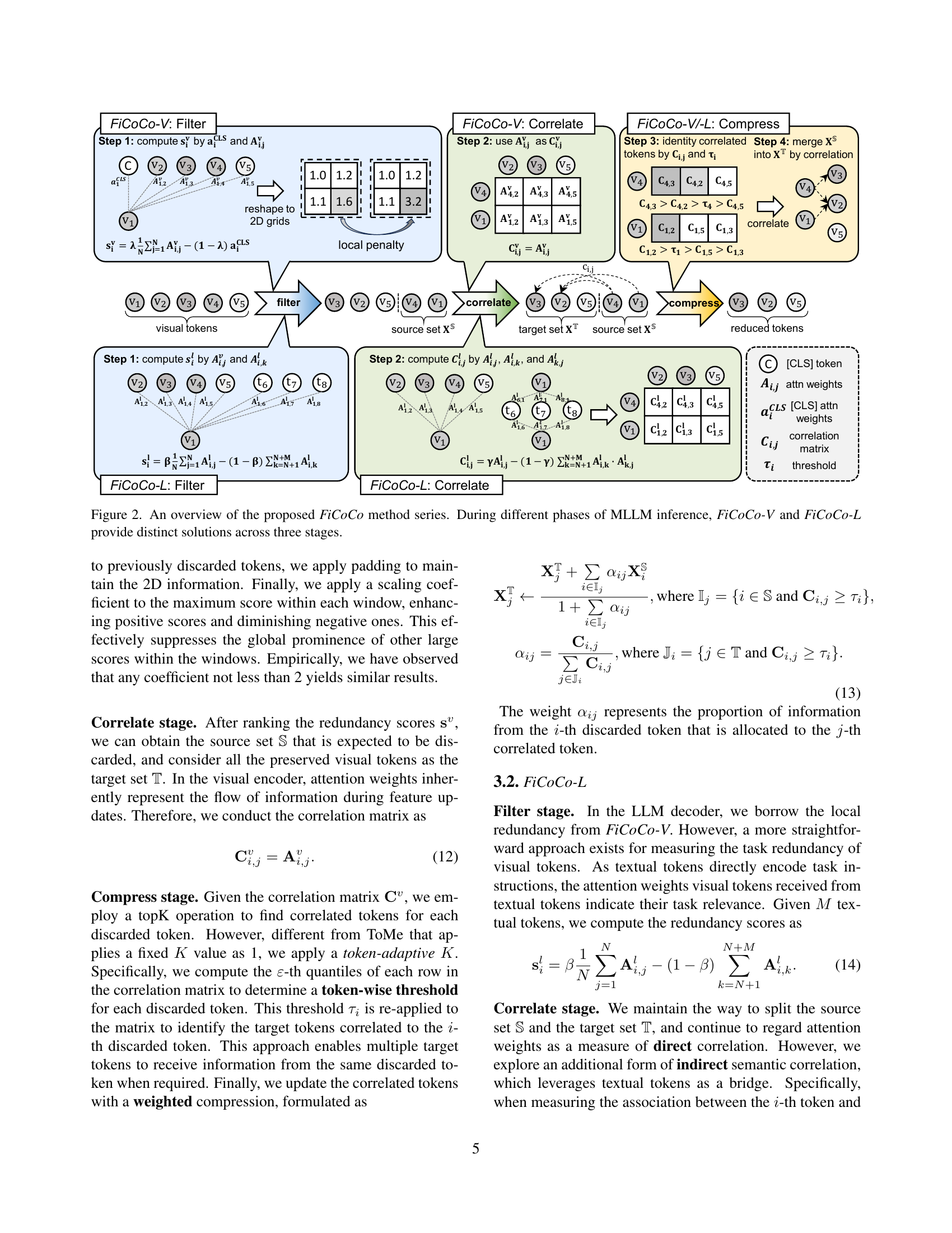
🔼 This figure illustrates the three-stage pipeline of the FiCoCo method series for training-free token reduction in Multimodal Large Language Models (MLLMs). It shows how FiCoCo-V and FiCoCo-L, which target the visual and language encoding phases respectively, each apply the filter, correlate, and compress stages. The filter stage identifies redundant tokens. The correlate stage establishes relationships between these and the preserved tokens. Finally, the compress stage integrates the redundant information into the preserved tokens. The figure visually depicts the flow and operations within each stage for both FiCoCo-V and FiCoCo-L, highlighting the differences in their approaches while maintaining a consistent structure across all three stages.
read the caption
Figure 2: An overview of the proposed FiCoCo method series. During different phases of MLLM inference, FiCoCo-V and FiCoCo-L provide distinct solutions across three stages.

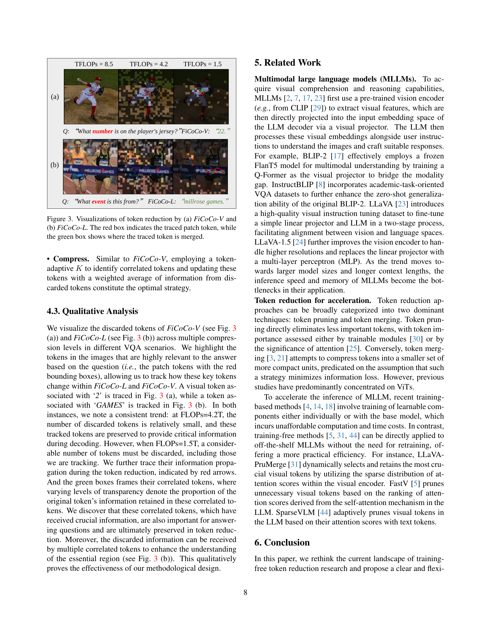
🔼 Figure 3 visualizes the effects of token reduction using FiCoCo-V and FiCoCo-L methods. In (a), FiCoCo-V’s token reduction is shown, highlighting how a key visual token (red box) is merged into another (green box). In (b), FiCoCo-L’s token reduction is presented, also demonstrating the merging of a key token (red box) with another token (green box). The process of token merging is tracked visually to show how important information is preserved. This qualitative analysis helps illustrate how the methods maintain relevant information during the reduction process, showing their effectiveness in reducing computational cost without significantly impacting accuracy.
read the caption
Figure 3: Visualizations of token reduction by (a) FiCoCo-V and (b) FiCoCo-L. The red box indicates the traced patch token, while the green box shows where the traced token is merged.

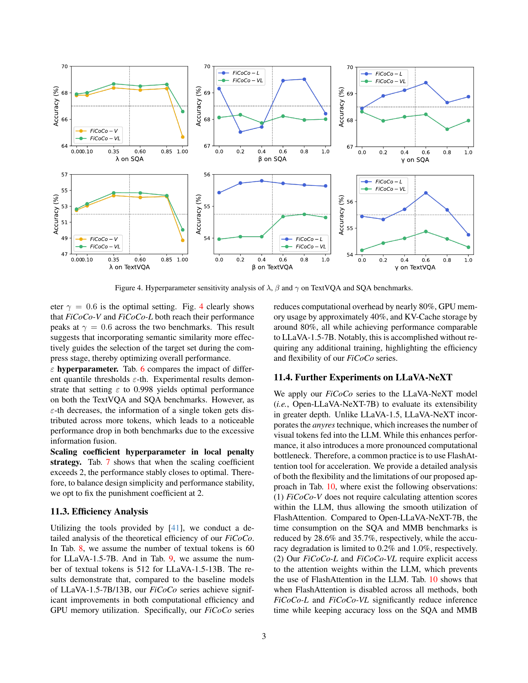
🔼 This figure displays the sensitivity analysis results for three hyperparameters (λ, β, and γ) used in the FiCoCo model. The analysis was performed on two benchmarks: TextVQA and SQA. Each subplot shows how changes in a specific hyperparameter affect the accuracy of the model on both benchmarks. The x-axis represents the value of the hyperparameter, while the y-axis represents the model’s accuracy. The plots provide insights into the optimal ranges and impact of these hyperparameters on the model’s performance, guiding hyperparameter tuning for improved results.
read the caption
Figure 4: Hyperparameter sensitivity analysis of λ𝜆\lambdaitalic_λ, β𝛽\betaitalic_β and γ𝛾\gammaitalic_γ on TextVQA and SQA benchmarks.
More on tables
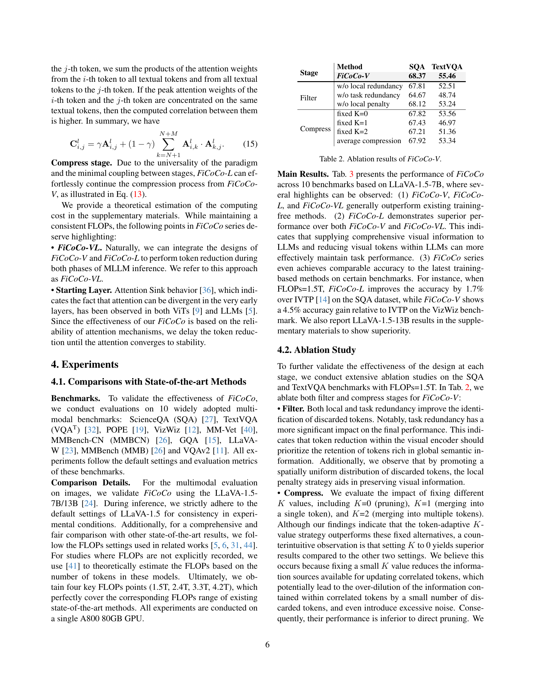
| Stage | Method | SQA | TextVQA |
|---|---|---|---|
| Stage | Method | SQA | TextVQA |
| FiCoCo-V | FiCoCo-V | 68.37 | 55.46 |
| Filter | w/o local redundancy | 67.81 | 52.51 |
| w/o task redundancy | 64.67 | 48.74 | |
| w/o local penalty | 68.12 | 53.24 | |
| Compress | fixed K=0 | 67.82 | 53.56 |
| fixed K=1 | 67.43 | 46.97 | |
| fixed K=2 | 67.21 | 51.36 | |
| average compression | 67.92 | 53.34 |
🔼 This table presents an ablation study on the FiCoCo-V model, showing the impact of different components on the model’s performance. It breaks down the results by examining the effects of removing the local redundancy calculation, task redundancy calculation, the local penalty strategy, and different fixed values for the hyperparameter K. This allows for a detailed analysis of each component’s contribution to the overall accuracy and efficiency of FiCoCo-V on the SQA and TextVQA benchmarks.
read the caption
Table 2: Ablation results of FiCoCo-V.
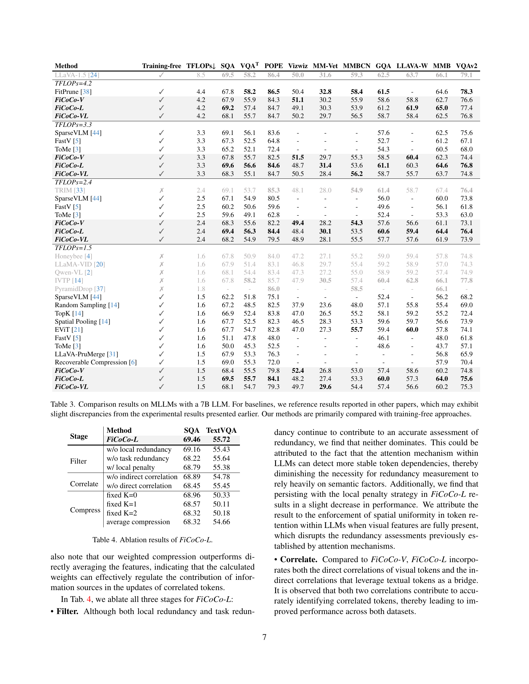
| Method | Training-free | TFLOPs↓ | SQA | VQAT | POPE | Vizwiz | MM-Vet | MMBCN | GQA | LLAVA-W | MMB | VQAv2 |
|---|---|---|---|---|---|---|---|---|---|---|---|---|
| LLaVA-1.5 [24] | ✓ | 8.5 | 69.5 | 58.2 | 86.4 | 50.0 | 31.6 | 59.3 | 62.5 | 63.7 | 66.1 | 79.1 |
| TFLOPs=4.2 | ||||||||||||
| FitPrune [38] | ✓ | 4.4 | 67.8 | 58.2 | 86.5 | 50.4 | 32.8 | 58.4 | 61.5 | - | 64.6 | 78.3 |
| FiCoCo-V | ✓ | 4.2 | 67.9 | 55.9 | 84.3 | 51.1 | 30.2 | 55.9 | 58.6 | 58.8 | 62.7 | 76.6 |
| FiCoCo-L | ✓ | 4.2 | 69.2 | 57.4 | 84.7 | 49.1 | 30.3 | 53.9 | 61.2 | 61.9 | 65.0 | 77.4 |
| FiCoCo-VL | ✓ | 4.2 | 68.1 | 55.7 | 84.7 | 50.2 | 29.7 | 56.5 | 58.7 | 58.4 | 62.5 | 76.8 |
| TFLOPs=3.3 | ||||||||||||
| SparseVLM [44] | ✓ | 3.3 | 69.1 | 56.1 | 83.6 | - | - | - | 57.6 | - | 62.5 | 75.6 |
| FastV [5] | ✓ | 3.3 | 67.3 | 52.5 | 64.8 | - | - | - | 52.7 | - | 61.2 | 67.1 |
| ToMe [3] | ✓ | 3.3 | 65.2 | 52.1 | 72.4 | - | - | - | 54.3 | - | 60.5 | 68.0 |
| FiCoCo-V | ✓ | 3.3 | 67.8 | 55.7 | 82.5 | 51.5 | 29.7 | 55.3 | 58.5 | 60.4 | 62.3 | 74.4 |
| FiCoCo-L | ✓ | 3.3 | 69.6 | 56.6 | 84.6 | 48.7 | 31.4 | 53.6 | 61.1 | 60.3 | 64.6 | 76.8 |
| FiCoCo-VL | ✓ | 3.3 | 68.3 | 55.1 | 84.7 | 50.5 | 28.4 | 56.2 | 58.7 | 55.7 | 63.7 | 74.8 |
| TFLOPs=2.4 | ||||||||||||
| TRIM [33] | ✗ | 2.4 | 69.1 | 53.7 | 85.3 | 48.1 | 28.0 | 54.9 | 61.4 | 58.7 | 67.4 | 76.4 |
| SparseVLM [44] | ✓ | 2.5 | 67.1 | 54.9 | 80.5 | - | - | - | 56.0 | - | 60.0 | 73.8 |
| FastV [5] | ✓ | 2.5 | 60.2 | 50.6 | 59.6 | - | - | - | 49.6 | - | 56.1 | 61.8 |
| ToMe [3] | ✓ | 2.5 | 59.6 | 49.1 | 62.8 | - | - | - | 52.4 | - | 53.3 | 63.0 |
| FiCoCo-V | ✓ | 2.4 | 68.3 | 55.6 | 82.2 | 49.4 | 28.2 | 54.3 | 57.6 | 56.6 | 61.1 | 73.1 |
| FiCoCo-L | ✓ | 2.4 | 69.4 | 56.3 | 84.4 | 48.4 | 30.1 | 53.5 | 60.6 | 59.4 | 64.4 | 76.4 |
| FiCoCo-VL | ✓ | 2.4 | 68.2 | 54.9 | 79.5 | 48.9 | 28.1 | 55.5 | 57.7 | 57.6 | 61.9 | 73.9 |
| TFLOPs=1.5 | ||||||||||||
| Honeybee [4] | ✗ | 1.6 | 67.8 | 50.9 | 84.0 | 47.2 | 27.1 | 55.2 | 59.0 | 59.4 | 57.8 | 74.8 |
| LLaMA-VID [20] | ✗ | 1.6 | 67.9 | 51.4 | 83.1 | 46.8 | 29.7 | 55.4 | 59.2 | 58.9 | 57.0 | 74.3 |
| Qwen-VL [2] | ✗ | 1.6 | 68.1 | 54.4 | 83.4 | 47.3 | 27.2 | 55.0 | 58.9 | 59.2 | 57.4 | 74.9 |
| IVTP [14] | ✗ | 1.6 | 67.8 | 58.2 | 85.7 | 47.9 | 30.5 | 57.4 | 60.4 | 62.8 | 66.1 | 77.8 |
| PyramidDrop [37] | ✗ | 1.8 | - | - | 86.0 | - | - | 58.5 | - | - | 66.1 | - |
| SparseVLM [44] | ✓ | 1.5 | 62.2 | 51.8 | 75.1 | - | - | - | 52.4 | - | 56.2 | 68.2 |
| Random Sampling [14] | ✓ | 1.6 | 67.2 | 48.5 | 82.5 | 37.9 | 23.6 | 48.0 | 57.1 | 55.8 | 55.4 | 69.0 |
| TopK [14] | ✓ | 1.6 | 66.9 | 52.4 | 83.8 | 47.0 | 26.5 | 55.2 | 58.1 | 59.2 | 55.2 | 72.4 |
| Spatial Pooling [14] | ✓ | 1.6 | 67.7 | 52.5 | 82.3 | 46.5 | 28.3 | 53.3 | 59.6 | 59.7 | 56.6 | 73.9 |
| EViT [21] | ✓ | 1.6 | 67.7 | 54.7 | 82.8 | 47.0 | 27.3 | 55.7 | 59.4 | 60.0 | 57.8 | 74.1 |
| FastV [5] | ✓ | 1.6 | 51.1 | 47.8 | 48.0 | - | - | - | 46.1 | - | 48.0 | 61.8 |
| ToMe [3] | ✓ | 1.6 | 50.0 | 45.3 | 52.5 | - | - | - | 48.6 | - | 43.7 | 57.1 |
| LLaVA-PruMerge [31] | ✓ | 1.5 | 67.9 | 53.3 | 76.3 | - | - | - | - | - | 56.8 | 65.9 |
| Recoverable Compression [6] | ✓ | 1.5 | 69.0 | 55.3 | 72.0 | - | - | - | - | - | 57.9 | 70.4 |
| FiCoCo-V | ✓ | 1.5 | 68.4 | 55.5 | 79.8 | 52.4 | 26.8 | 53.0 | 57.4 | 58.6 | 60.2 | 74.8 |
| FiCoCo-L | ✓ | 1.5 | 69.5 | 55.7 | 84.1 | 48.2 | 27.4 | 53.3 | 60.0 | 57.3 | 64.0 | 75.6 |
| FiCoCo-VL | ✓ | 1.5 | 68.1 | 54.7 | 79.3 | 49.7 | 29.6 | 54.4 | 57.4 | 56.6 | 60.2 | 75.3 |
🔼 This table presents a comparison of the performance of various methods for accelerating multimodal large language models (MLLMs), specifically focusing on models with 7 billion parameters. It shows the results across ten different benchmark datasets, comparing the performance (accuracy) and computational cost (TFLOPs) of different approaches. The baselines include several existing methods from the literature, while the authors’ methods (FiCoCo-V, FiCoCo-L, and FiCoCo-VL) are also included. Note that because the baselines come from different publications, there might be small variations in reported performance numbers due to differences in experimental setups. The table primarily compares the authors’ methods with other training-free techniques, meaning methods that do not require retraining the model to achieve speed improvements.
read the caption
Table 3: Comparison results on MLLMs with a 7B LLM. For baselines, we reference results reported in other papers, which may exhibit slight discrepancies from the experimental results presented earlier. Our methods are primarily compared with training-free approaches.
| Stage | Method | SQA | TextVQA |
|---|---|---|---|
| Stage | Method | SQA | TextVQA |
| FiCoCo-L | FiCoCo-L | 69.46 | 55.72 |
| Filter | w/o local redundancy | 69.16 | 55.43 |
| w/o task redundancy | 68.22 | 55.64 | |
| w/ local penalty | 68.79 | 55.38 | |
| Correlate | w/o indirect correlation | 68.89 | 54.78 |
| w/o direct correlation | 68.45 | 55.45 | |
| Compress | fixed K=0 | 68.96 | 50.33 |
| fixed K=1 | 68.57 | 50.11 | |
| fixed K=2 | 68.32 | 50.18 | |
| average compression | 68.32 | 54.66 |
🔼 This table presents the ablation study results for the FiCoCo-L model, demonstrating the impact of removing different components on the model’s performance. It analyzes the contribution of each of the three stages (Filter, Correlate, and Compress) and various design choices within those stages on two benchmark datasets, SQA and TextVQA. The results show the effect of removing or modifying elements such as local and task redundancy in the Filter stage, direct and indirect correlation in the Correlate stage, and different compression strategies (e.g., fixed K-values versus adaptive K) in the Compress stage. The table aims to provide a detailed understanding of the individual components’ contribution to the overall model performance.
read the caption
Table 4: Ablation results of FiCoCo-L.
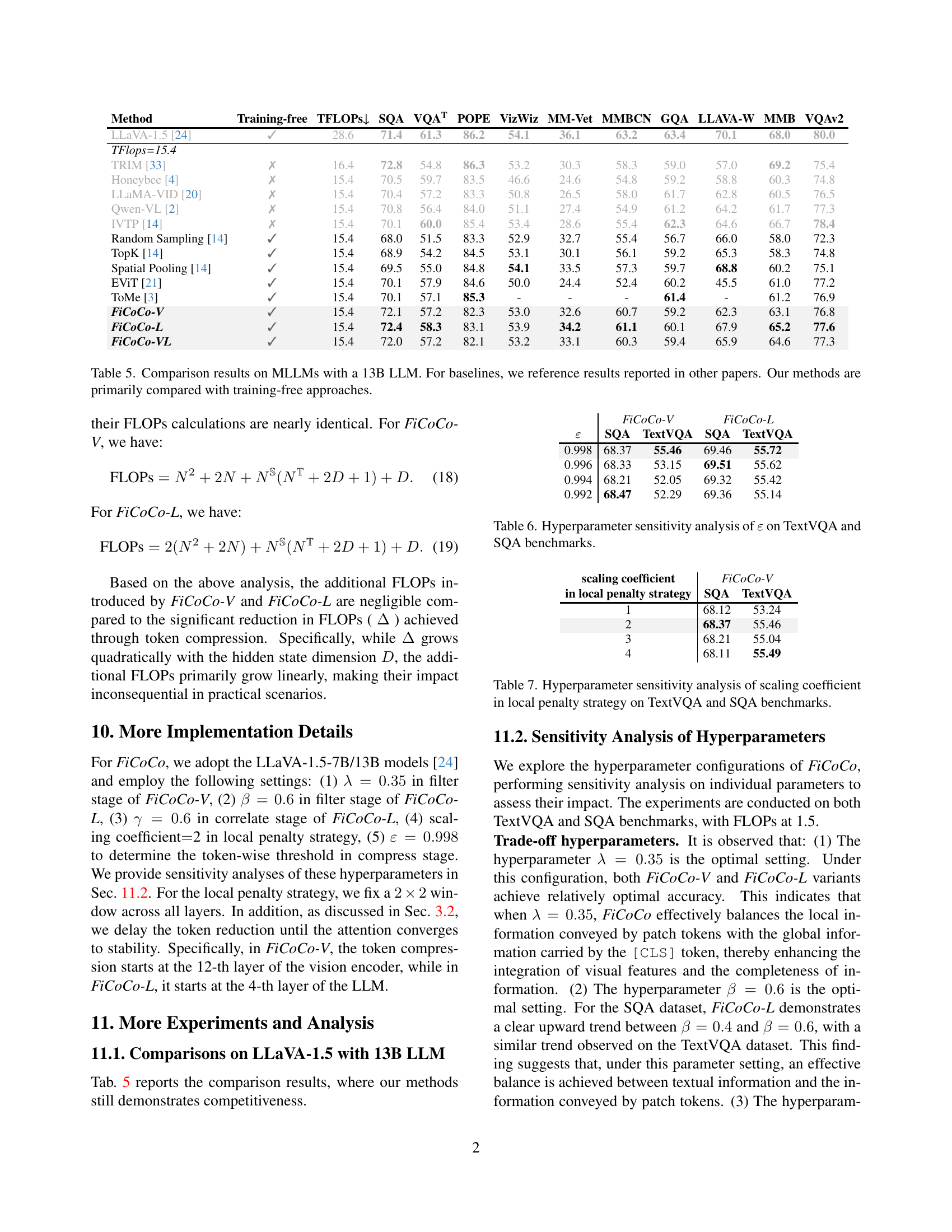
| Method | Training-free | TFLOPs↓ | SQA | VQAT | POPE | VizWiz | MM-Vet | MMBCN | GQA | LLAVA-W | MMB | VQAv2 |
|---|---|---|---|---|---|---|---|---|---|---|---|---|
| LLaVA-1.5 [24] | ✓ | 28.6 | 71.4 | 61.3 | 86.2 | 54.1 | 36.1 | 63.2 | 63.4 | 70.1 | 68.0 | 80.0 |
| TFlops=15.4 | ||||||||||||
| TRIM [33] | ✗ | 16.4 | 72.8 | 54.8 | 86.3 | 53.2 | 30.3 | 58.3 | 59.0 | 57.0 | 69.2 | 75.4 |
| Honeybee [4] | ✗ | 15.4 | 70.5 | 59.7 | 83.5 | 46.6 | 24.6 | 54.8 | 59.2 | 58.8 | 60.3 | 74.8 |
| LLaMA-VID [20] | ✗ | 15.4 | 70.4 | 57.2 | 83.3 | 50.8 | 26.5 | 58.0 | 61.7 | 62.8 | 60.5 | 76.5 |
| Qwen-VL [2] | ✗ | 15.4 | 70.8 | 56.4 | 84.0 | 51.1 | 27.4 | 54.9 | 61.2 | 64.2 | 61.7 | 77.3 |
| IVTP [14] | ✗ | 15.4 | 70.1 | 60.0 | 85.4 | 53.4 | 28.6 | 55.4 | 62.3 | 64.6 | 66.7 | 78.4 |
| Random Sampling [14] | ✓ | 15.4 | 68.0 | 51.5 | 83.3 | 52.9 | 32.7 | 55.4 | 56.7 | 66.0 | 58.0 | 72.3 |
| TopK [14] | ✓ | 15.4 | 68.9 | 54.2 | 84.5 | 53.1 | 30.1 | 56.1 | 59.2 | 65.3 | 58.3 | 74.8 |
| Spatial Pooling [14] | ✓ | 15.4 | 69.5 | 55.0 | 84.8 | 54.1 | 33.5 | 57.3 | 59.7 | 68.8 | 60.2 | 75.1 |
| EViT [21] | ✓ | 15.4 | 70.1 | 57.9 | 84.6 | 50.0 | 24.4 | 52.4 | 60.2 | 45.5 | 61.0 | 77.2 |
| ToMe [3] | ✓ | 15.4 | 70.1 | 57.1 | 85.3 | - | - | - | 61.4 | - | 61.2 | 76.9 |
| FiCoCo-V | ✓ | 15.4 | 72.1 | 57.2 | 82.3 | 53.0 | 32.6 | 60.7 | 59.2 | 62.3 | 63.1 | 76.8 |
| FiCoCo-L | ✓ | 15.4 | 72.4 | 58.3 | 83.1 | 53.9 | 34.2 | 61.1 | 60.1 | 67.9 | 65.2 | 77.6 |
| FiCoCo-VL | ✓ | 15.4 | 72.0 | 57.2 | 82.1 | 53.2 | 33.1 | 60.3 | 59.4 | 65.9 | 64.6 | 77.3 |
🔼 Table 5 presents a detailed comparison of various methods’ performance on multimodal large language models (MLLMs) using a 13B parameter LLM. It showcases the accuracy achieved by different techniques across ten widely-used benchmark datasets. The table highlights the trade-off between computational efficiency (measured in TeraFLOPs) and accuracy. A key aspect of the table is its focus on comparing training-free methods against existing methods. This is crucial because training-free methods offer a more practical and accessible approach for accelerating the inference of these large models. The results allow for direct comparison between the proposed FiCoCo methods and existing state-of-the-art techniques, demonstrating the effectiveness of the proposed approaches.
read the caption
Table 5: Comparison results on MLLMs with a 13B LLM. For baselines, we reference results reported in other papers. Our methods are primarily compared with training-free approaches.
| FiCoCo-V | FiCoCo-L | |
|---|---|---|
| ε | SQA | TextVQA |
| — | — | — |
| 0.998 | 68.37 | 55.46 |
| 0.996 | 68.33 | 53.15 |
| 0.994 | 68.21 | 52.05 |
| 0.992 | 68.47 | 52.29 |
🔼 This table presents the results of an ablation study evaluating the impact of the hyperparameter ε (epsilon) on the performance of the FiCoCo model. Epsilon controls the threshold for determining which tokens are considered correlated during the compression stage. The table shows how varying epsilon affects the accuracy on two benchmarks: TextVQA and SQA, indicating the optimal setting for epsilon that balances efficiency and accuracy.
read the caption
Table 6: Hyperparameter sensitivity analysis of ε𝜀\varepsilonitalic_ε on TextVQA and SQA benchmarks.
| scaling coefficient | FiCoCo-V | SQA | TextVQA |
|---|---|---|---|
| in local penalty strategy | FiCoCo-V | SQA | TextVQA |
| 1 | 68.12 | 53.24 | |
| 2 | 68.37 | 55.46 | |
| 3 | 68.21 | 55.04 | |
| 4 | 68.11 | 55.49 |
🔼 This table presents the results of an ablation study investigating the impact of the scaling coefficient hyperparameter used in the local penalty strategy within the FiCoCo-V method. The study evaluates performance on two benchmarks: TextVQA and SQA. Different scaling coefficient values are tested to determine their effect on model accuracy. The goal is to identify the optimal balance between preventing spatial-centralized information loss and achieving efficient performance.
read the caption
Table 7: Hyperparameter sensitivity analysis of scaling coefficient in local penalty strategy on TextVQA and SQA benchmarks.
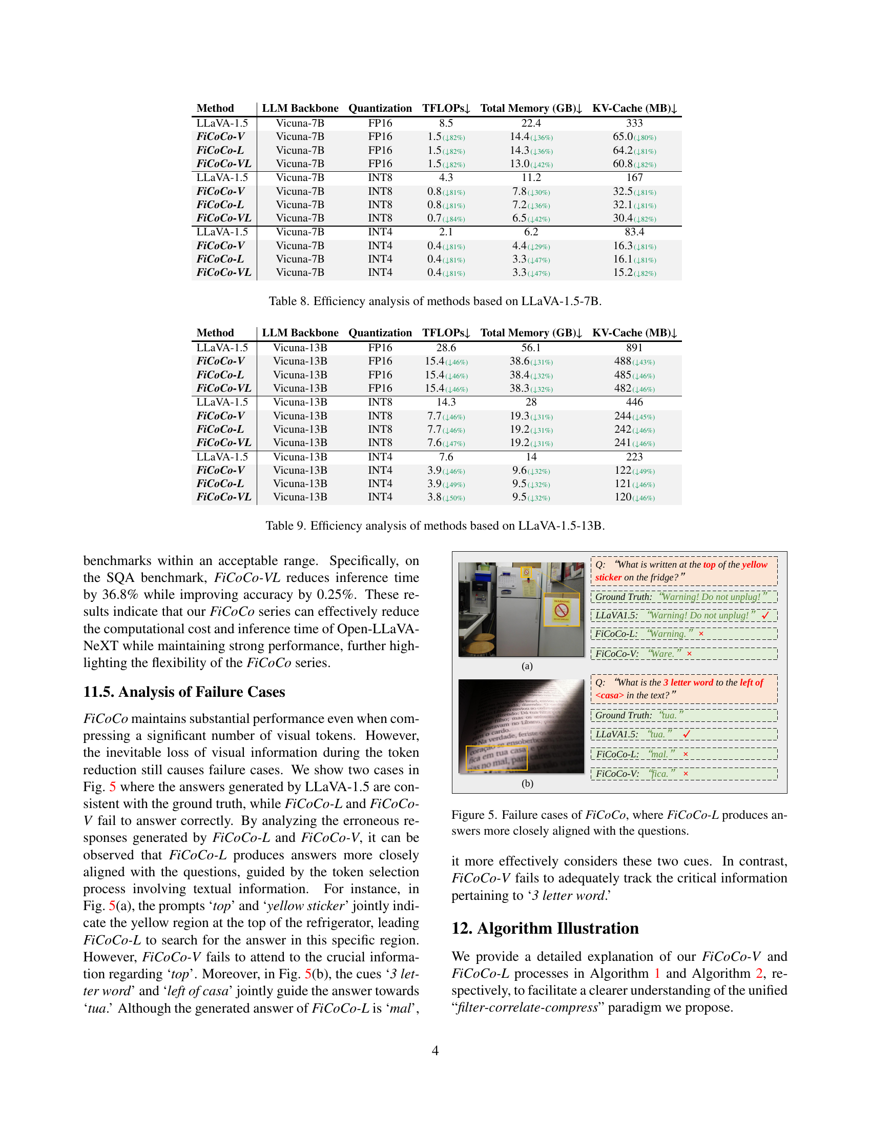
| Method | LLM Backbone | Quantization | TFLOPs↓ | Total Memory (GB)↓ | KV-Cache (MB)↓ |
|---|---|---|---|---|---|
| LLaVA-1.5 | Vicuna-7B | FP16 | 8.5 | 22.4 | 333 |
| FiCoCo-V | Vicuna-7B | FP16 | 1.5 (↓82%) | 14.4 (↓36%) | 65.0 (↓80%) |
| FiCoCo-L | Vicuna-7B | FP16 | 1.5 (↓82%) | 14.3 (↓36%) | 64.2 (↓81%) |
| FiCoCo-VL | Vicuna-7B | FP16 | 1.5 (↓82%) | 13.0 (↓42%) | 60.8 (↓82%) |
| LLaVA-1.5 | Vicuna-7B | INT8 | 4.3 | 11.2 | 167 |
| FiCoCo-V | Vicuna-7B | INT8 | 0.8 (↓81%) | 7.8 (↓30%) | 32.5 (↓81%) |
| FiCoCo-L | Vicuna-7B | INT8 | 0.8 (↓81%) | 7.2 (↓36%) | 32.1 (↓81%) |
| FiCoCo-VL | Vicuna-7B | INT8 | 0.7 (↓84%) | 6.5 (↓42%) | 30.4 (↓82%) |
| LLaVA-1.5 | Vicuna-7B | INT4 | 2.1 | 6.2 | 83.4 |
| FiCoCo-V | Vicuna-7B | INT4 | 0.4 (↓81%) | 4.4 (↓29%) | 16.3 (↓81%) |
| FiCoCo-L | Vicuna-7B | INT4 | 0.4 (↓81%) | 3.3 (↓47%) | 16.1 (↓81%) |
| FiCoCo-VL | Vicuna-7B | INT4 | 0.4 (↓81%) | 3.3 (↓47%) | 15.2 (↓82%) |
🔼 This table presents a detailed efficiency analysis of various methods for accelerating inference in Multimodal Large Language Models (MLLMs), specifically using the LLaVA-1.5-7B model. It compares the original LLaVA-1.5 model with three variants of the FiCoCo method (FiCoCo-V, FiCoCo-L, FiCoCo-VL) under different quantization levels (FP16, INT8, INT4). The metrics presented include total inference time (TFLOPs), total memory usage (GB), and KV-Cache usage (MB). This allows for a comprehensive comparison of the efficiency gains achieved by FiCoCo in reducing computational cost and memory requirements while maintaining performance.
read the caption
Table 8: Efficiency analysis of methods based on LLaVA-1.5-7B.
| Method | LLM Backbone | Quantization | TFLOPs↓ | Total Memory (GB)↓ | KV-Cache (MB)↓ |
|---|---|---|---|---|---|
| LLaVA-1.5 | Vicuna-13B | FP16 | 28.6 | 56.1 | 891 |
| FiCoCo-V | Vicuna-13B | FP16 | 15.4 (↓46%) | 38.6 (↓31%) | 488 (↓43%) |
| FiCoCo-L | Vicuna-13B | FP16 | 15.4 (↓46%) | 38.4 (↓32%) | 485 (↓46%) |
| FiCoCo-VL | Vicuna-13B | FP16 | 15.4 (↓46%) | 38.3 (↓32%) | 482 (↓46%) |
| LLaVA-1.5 | Vicuna-13B | INT8 | 14.3 | 28 | 446 |
| FiCoCo-V | Vicuna-13B | INT8 | 7.7 (↓46%) | 19.3 (↓31%) | 244 (↓45%) |
| FiCoCo-L | Vicuna-13B | INT8 | 7.7 (↓46%) | 19.2 (↓31%) | 242 (↓46%) |
| FiCoCo-VL | Vicuna-13B | INT8 | 7.6 (↓47%) | 19.2 (↓31%) | 241 (↓46%) |
| LLaVA-1.5 | Vicuna-13B | INT4 | 7.6 | 14 | 223 |
| FiCoCo-V | Vicuna-13B | INT4 | 3.9 (↓46%) | 9.6 (↓32%) | 122 (↓49%) |
| FiCoCo-L | Vicuna-13B | INT4 | 3.9 (↓49%) | 9.5 (↓32%) | 121 (↓46%) |
| FiCoCo-VL | Vicuna-13B | INT4 | 3.8 (↓50%) | 9.5 (↓32%) | 120 (↓46%) |
🔼 This table presents a comprehensive efficiency analysis of various methods, including the proposed FiCoCo variants, using the LLaVA-1.5-13B model as the base. It compares the performance of these methods across different quantization levels (FP16, INT8, INT4), showing the trade-offs between computational cost (TFLOPs), total memory usage, and KV-cache size. The results highlight the efficiency gains achieved by FiCoCo in reducing computational cost and memory footprint while maintaining comparable accuracy.
read the caption
Table 9: Efficiency analysis of methods based on LLaVA-1.5-13B.
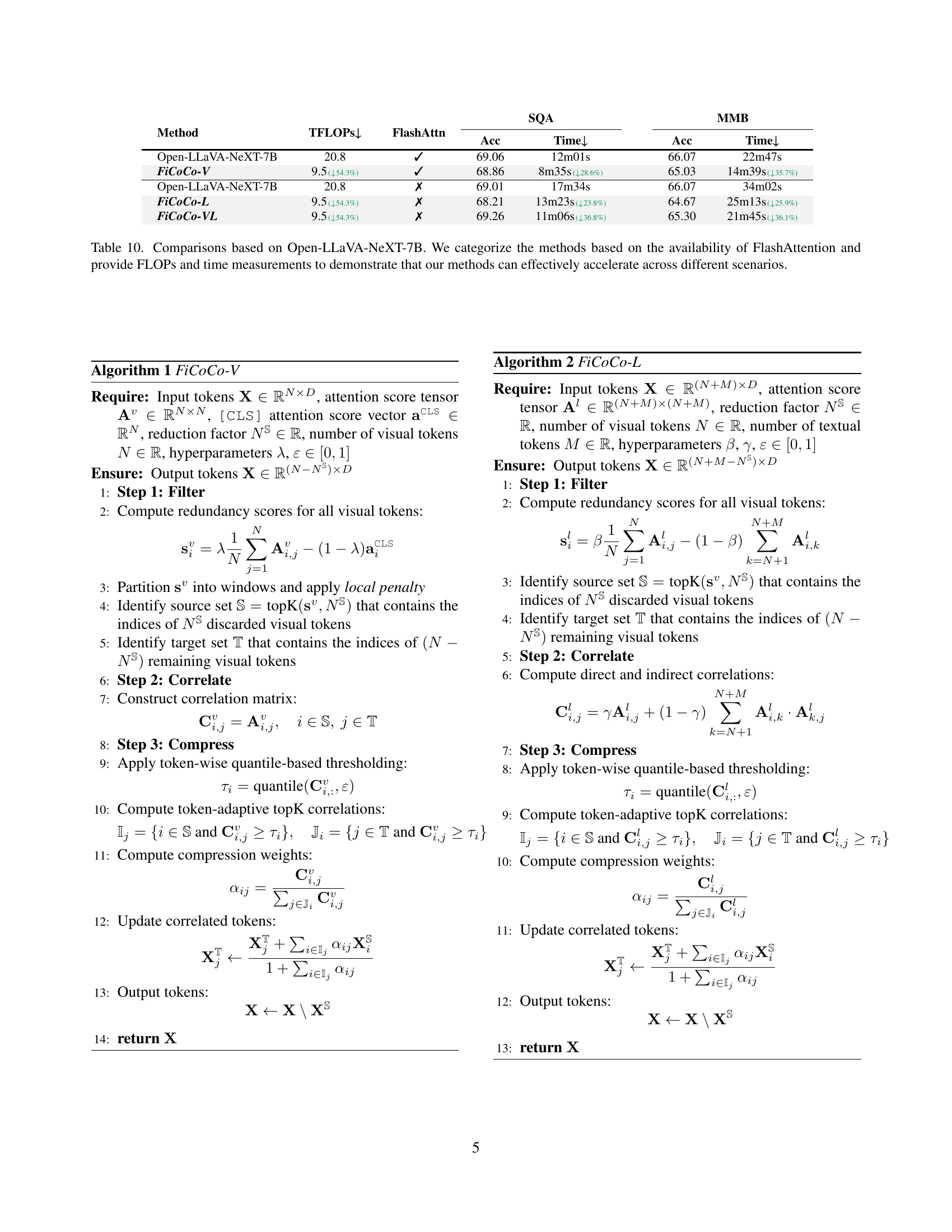
| Method | TFLOPs↓ | FlashAttn | SQA Acc | SQA Time↓ | MMB Acc | MMB Time↓ | |
|---|---|---|---|---|---|---|---|
| Open-LLaVA-NeXT-7B | 20.8 | ✓ | 69.06 | 12m01s | 66.07 | 22m47s | |
| FiCoCo-V | 9.5 (↓54.3%) | ✓ | 68.86 | 8m35s (↓28.6%) | 65.03 | 14m39s (↓35.7%) | |
| Open-LLaVA-NeXT-7B | 20.8 | ✗ | 69.01 | 17m34s | 66.07 | 34m02s | |
| FiCoCo-L | 9.5 (↓54.3%) | ✗ | 68.21 | 13m23s (↓23.8%) | 64.67 | 25m13s (↓25.9%) | |
| FiCoCo-VL | 9.5 (↓54.3%) | ✗ | 69.26 | 11m06s (↓36.8%) | 65.30 | 21m45s (↓36.1%) |
🔼 This table presents a comparison of performance metrics for different models on the Open-LLaVA-NeXT-7B benchmark. The models are categorized based on whether they utilize FlashAttention, a technique for accelerating inference. The key performance indicators (KPIs) presented include FLOPs (floating-point operations), inference time, and accuracy on two specific benchmarks (SQA and MMB). The purpose of the table is to demonstrate that the proposed FiCoCo methods effectively improve efficiency across various scenarios, even when using or not using FlashAttention.
read the caption
Table 10: Comparisons based on Open-LLaVA-NeXT-7B. We categorize the methods based on the availability of FlashAttention and provide FLOPs and time measurements to demonstrate that our methods can effectively accelerate across different scenarios.
Full paper#
