↗ arXiv ↗ Hugging Face ↗ Papers with Code
TL;DR#
Visual Auto-Regressive (VAR) models, while efficient for image generation, suffer from high memory consumption and computational costs due to their coarse-to-fine prediction process resulting in long token sequences. This limits their scalability and real-world applicability.
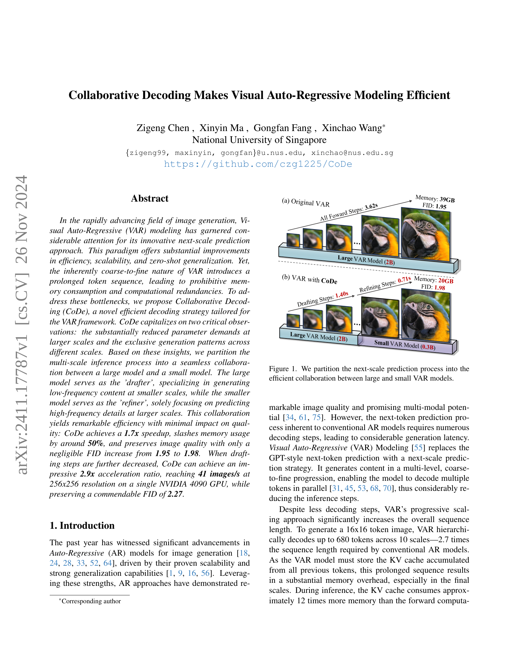
The proposed Collaborative Decoding (CoDe) addresses these issues. CoDe partitions the multi-scale inference into a collaboration between a large and a small model. The large model generates low-frequency content, while the small model refines high-frequency details. This division significantly reduces computational redundancy and parameter demands, leading to substantial improvements in efficiency without sacrificing image quality. CoDe achieves a 1.7x speedup and 50% memory reduction compared to the original VAR model, establishing a new benchmark for efficient high-quality image generation.
Key Takeaways#
Why does it matter?#
This paper is important because it presents a novel and efficient decoding strategy for visual auto-regressive (VAR) models, a rapidly advancing field in image generation. By significantly reducing memory usage and computational costs while maintaining image quality, CoDe offers a practical solution to a key challenge in VAR modeling, paving the way for more efficient and scalable image generation systems. The work also inspires further research into efficient decoding strategies and specialized model training for improved resource utilization in other deep learning models. This could lead to breakthroughs in a wide range of applications including, but not limited to, image generation and editing, and other high-resolution tasks that require extensive computational resources.
Visual Insights#
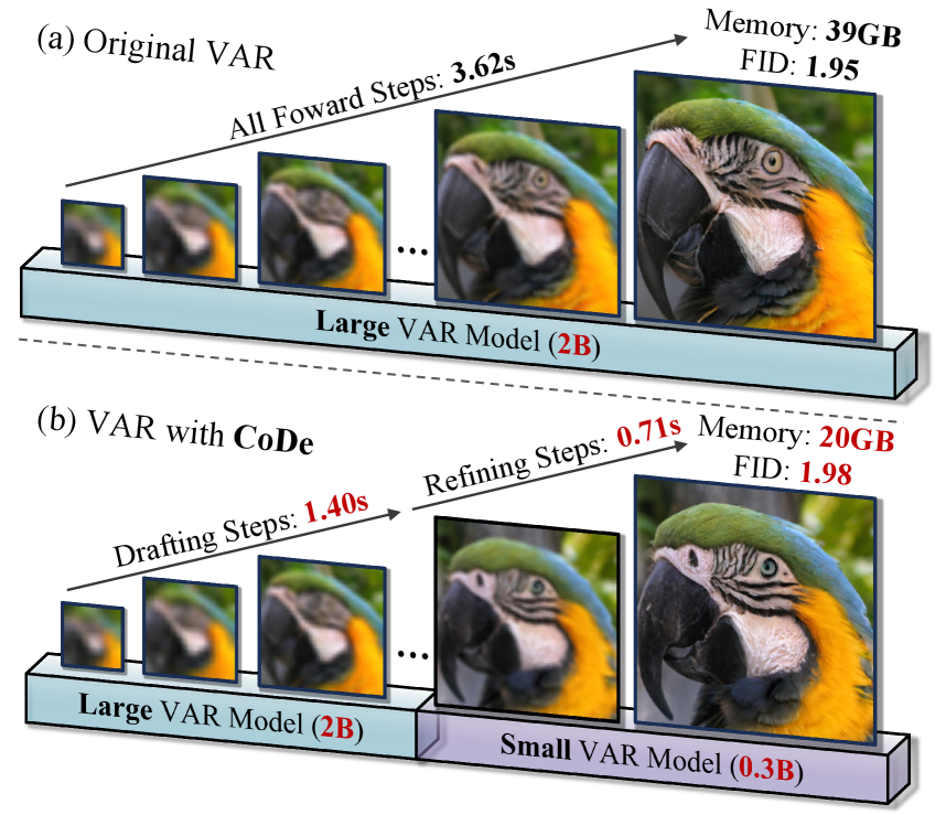
🔼 This figure illustrates the core concept of Collaborative Decoding (CoDe). The original Visual Autoregressive (VAR) model’s next-scale prediction process is computationally expensive due to the lengthy token sequence involved. CoDe addresses this by dividing the process into two collaborative stages. A larger VAR model (2B parameters) acts as the ‘drafter’, generating low-frequency content at smaller scales quickly. A smaller VAR model (0.3B parameters) acts as the ‘refiner’, focusing on predicting high-frequency details at larger scales. This collaboration reduces computational redundancy and memory usage without significant quality loss, resulting in increased efficiency. The figure visually shows the parallel processing of drafting and refining steps in the multi-scale inference process, showcasing the time and memory savings achieved by CoDe compared to the traditional VAR approach.
read the caption
Figure 1: We partition the next-scale prediction process into the efficient collaboration between large and small VAR models.
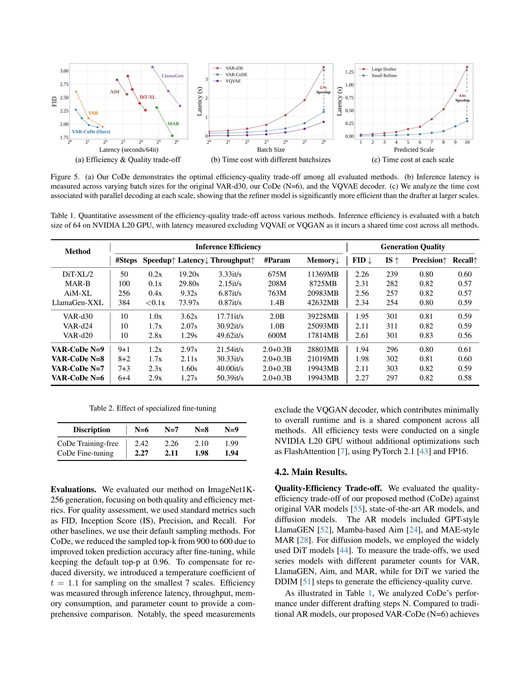
| Method | #Steps | Speedup↑ | Latency↓ | Throughput↑ | #Param | Memory↓ | FID↓ | IS↑ | Precision↑ | Recall↑ |
|---|---|---|---|---|---|---|---|---|---|---|
| DiT-XL/2 | 50 | 0.2x | 19.20s | 3.33it/s | 675M | 11369MB | 2.26 | 239 | 0.80 | 0.60 |
| MAR-B | 100 | 0.1x | 29.80s | 2.15it/s | 208M | 8725MB | 2.31 | 282 | 0.82 | 0.57 |
| AiM-XL | 256 | 0.4x | 9.32s | 6.87it/s | 763M | 20983MB | 2.56 | 257 | 0.82 | 0.57 |
| LlamaGen-XXL | 384 | <0.1x | 73.97s | 0.87it/s | 1.4B | 42632MB | 2.34 | 254 | 0.80 | 0.59 |
| VAR-d30 | 10 | 1.0x | 3.62s | 17.71it/s | 2.0B | 39228MB | 1.95 | 301 | 0.81 | 0.59 |
| VAR-d24 | 10 | 1.7x | 2.07s | 30.92it/s | 1.0B | 25093MB | 2.11 | 311 | 0.82 | 0.59 |
| VAR-d20 | 10 | 2.8x | 1.29s | 49.62it/s | 600M | 17814MB | 2.61 | 301 | 0.83 | 0.56 |
| VAR-CoDe N=9 | 9+1 | 1.2x | 2.97s | 21.54it/s | 2.0+0.3B | 28803MB | 1.94 | 296 | 0.80 | 0.61 |
| VAR-CoDe N=8 | 8+2 | 1.7x | 2.11s | 30.33it/s | 2.0+0.3B | 21019MB | 1.98 | 302 | 0.81 | 0.60 |
| VAR-CoDe N=7 | 7+3 | 2.3x | 1.60s | 40.00it/s | 2.0+0.3B | 19943MB | 2.11 | 303 | 0.82 | 0.59 |
| VAR-CoDe N=6 | 6+4 | 2.9x | 1.27s | 50.39it/s | 2.0+0.3B | 19943MB | 2.27 | 297 | 0.82 | 0.58 |
🔼 This table presents a comparison of different image generation methods based on their efficiency and image quality. Efficiency is measured by speedup (relative to a baseline method), latency (inference time), and throughput (images generated per second). Image quality is assessed using FID (Fréchet Inception Distance), Inception Score (IS), precision, and recall. The experiments were conducted with a batch size of 64 on an NVIDIA L20 GPU, and the latency measurements exclude the time taken by VQGAN or VQVAE decoders as these are shared across all methods.
read the caption
Table 1: Quantitative assessment of the efficiency-quality trade-off across various methods. Inference efficiency is evaluated with a batch size of 64 on NVIDIA L20 GPU, with latency measured excluding VQVAE or VQGAN as it incurs a shared time cost across all methods.
In-depth insights#
CoDe: VAR Efficiency#
The core of CoDe lies in improving the efficiency of Visual Autoregressive (VAR) models for image generation. CoDe cleverly partitions the multi-scale inference process into a collaborative effort between a large and a small VAR model. The large model acts as a ‘drafter,’ efficiently generating low-frequency content at initial scales, while the smaller model refines high-frequency details at larger scales. This division of labor significantly reduces computational redundancy, as larger models are less crucial for later stages. Experimental results demonstrate that CoDe achieves a substantial speedup (up to 2.9x) and memory reduction (~50%) with only a negligible impact on image quality. The success of CoDe highlights the effectiveness of a specialized, collaborative approach to address the inherent computational bottlenecks of VAR models, paving the way for more efficient high-resolution image generation.
Multi-Scale Collab#
The concept of “Multi-Scale Collab” in visual autoregressive modeling suggests a synergistic approach where models of different scales collaborate to enhance efficiency and image quality. A large model might focus on drafting the low-frequency, global structure of the image at coarser scales, acting as a ‘drafter’. Simultaneously, a smaller model, excelling at high-frequency details, refines the image at finer scales, taking on the role of a ‘refiner’. This division of labor leverages the observation that parameter demands decrease as scales increase, allowing for efficient resource allocation. Furthermore, this strategy addresses the exclusive generation patterns across scales, mitigating the interference often found when a single model tries to handle both low and high-frequency information. Fine-tuning each model on its designated scale further enhances specialization and minimizes training conflicts, ultimately improving generation speed and image quality while reducing computational burden. The success of this method hinges on the proper balance between drafting and refining steps and the selection of appropriately sized models for optimal performance. Training-free collaboration is also possible, showcasing the flexibility of the approach.
Specialized FT#
The heading ‘Specialized FT’, likely referring to ‘Specialized Fine-Tuning’, highlights a crucial innovation in the paper. Instead of jointly training a single model for all scales in visual autoregressive (VAR) modeling, this technique independently fine-tunes the ‘drafter’ (large model) and ‘refiner’ (small model) on their respective scales. This addresses the inherent interference between low- and high-frequency feature learning present in traditional VAR training. By isolating training to specific frequency ranges, the method enhances parameter utilization efficiency and improves the model’s capacity to learn distinct features at each scale. This approach is particularly effective given the observation that larger scales require fewer parameters for high-quality generation. The results strongly suggest that this specialized fine-tuning is not merely additive but synergistically improves the speed and efficiency of inference compared to approaches using training-free collaboration or single model training. Furthermore, it mitigates the detrimental effects of conflicting training signals that compromise overall model performance. In essence, ‘Specialized FT’ is key to CoDe’s superior efficiency without substantial quality degradation.
CoDe Limits#
The effectiveness of Collaborative Decoding (CoDe) hinges on the successful collaboration between a large and a small model. A critical limitation is the necessity of having two models, which might be impractical or computationally expensive depending on resource constraints. The approach also requires careful consideration of the number of drafting and refining steps (N), as an imbalanced allocation could compromise efficiency or image quality. While CoDe significantly improves upon traditional methods, it introduces additional complexity in model training and deployment, demanding specialized fine-tuning for optimal performance. Furthermore, the method’s scalability to even higher resolutions and different image modalities requires further investigation. Although CoDe excels in accelerating inference and reducing memory usage, achieving a perfect balance of speed and quality warrants further exploration and optimization.
Future Works#
The ‘Future Work’ section of this research paper on Collaborative Decoding (CoDe) for efficient visual auto-regressive modeling presents exciting avenues for improvement and expansion. High-resolution image generation is a primary target, as CoDe’s efficiency gains become more pronounced with increased resolution. Exploring model architectures beyond the current transformer-based setup is crucial, potentially leading to even greater efficiency. Incorporating CoDe into other autoregressive tasks such as video generation is a natural extension. Additionally, researching techniques to further streamline the training process for the separate drafter and refiner models, perhaps via knowledge distillation or efficient parameter transfer, is key to enhancing the overall practicality of CoDe. Finally, a thorough investigation into the trade-offs between speed, memory usage, and image quality across various model sizes and drafting step configurations would provide a more complete understanding of CoDe’s performance landscape.
More visual insights#
More on figures

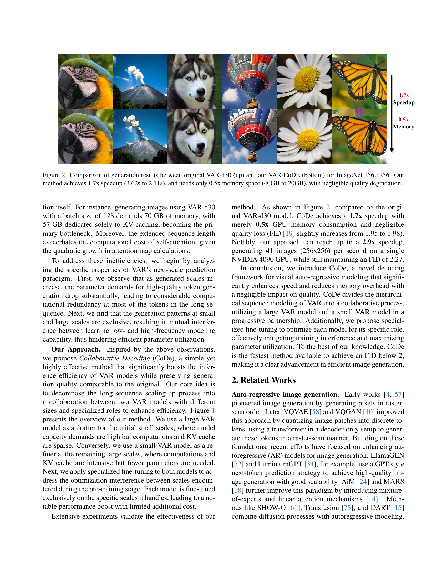
🔼 This figure compares image generation results between the original VAR-d30 model and the proposed VAR-CoDe model on the ImageNet 256x256 dataset. The top row shows images generated using the original VAR-d30 model, highlighting its generation time of 3.62 seconds and memory usage of 40GB. The bottom row displays images generated by the VAR-CoDe method, demonstrating a 1.7x speedup (2.11 seconds) and a 50% reduction in memory usage (20GB). Importantly, the visual quality remains almost identical between the two methods, indicating negligible quality degradation due to the efficiency improvements achieved by VAR-CoDe.
read the caption
Figure 2: Comparison of generation results between original VAR-d30 (up) and our VAR-CoDE (bottom) for ImageNet 256×\times×256. Our method achieves 1.7x speedup (3.62s to 2.11s), and needs only 0.5x memory space (40GB to 20GB), with negligible quality degradation.

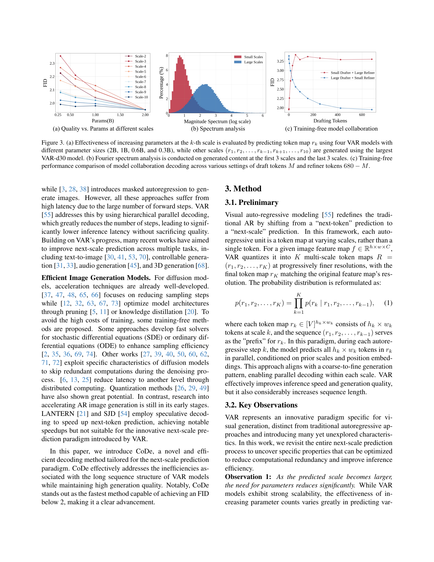
🔼 Figure 3 demonstrates three key aspects of the Collaborative Decoding (CoDe) method. (a) It shows that increasing model parameters is more effective in improving the quality of generated content at smaller scales than at larger scales. This is done by using different sized models to generate tokens at different scales. (b) Fourier analysis shows that smaller scales generate low-frequency information, while larger scales generate high-frequency detail. (c) Shows the effect of varying the number of drafting and refining tokens on the final model’s performance.
read the caption
Figure 3: (a) Effectiveness of increasing parameters at the k𝑘kitalic_k-th scale is evaluated by predicting token map rksubscript𝑟𝑘r_{k}italic_r start_POSTSUBSCRIPT italic_k end_POSTSUBSCRIPT using four VAR models with different parameter sizes (2B, 1B, 0.6B, and 0.3B), while other scales (r1,r2,…,rk−1,rk+1,…,r10)subscript𝑟1subscript𝑟2…subscript𝑟𝑘1subscript𝑟𝑘1…subscript𝑟10(r_{1},r_{2},\dots,r_{k-1},r_{k+1},\dots,r_{10})( italic_r start_POSTSUBSCRIPT 1 end_POSTSUBSCRIPT , italic_r start_POSTSUBSCRIPT 2 end_POSTSUBSCRIPT , … , italic_r start_POSTSUBSCRIPT italic_k - 1 end_POSTSUBSCRIPT , italic_r start_POSTSUBSCRIPT italic_k + 1 end_POSTSUBSCRIPT , … , italic_r start_POSTSUBSCRIPT 10 end_POSTSUBSCRIPT ) are generated using the largest VAR-d30 model. (b) Fourier spectrum analysis is conducted on generated content at the first 3 scales and the last 3 scales. (c) Training-free performance comparison of model collaboration decoding across various settings of draft tokens M𝑀Mitalic_M and refiner tokens 680−M680𝑀680-M680 - italic_M.

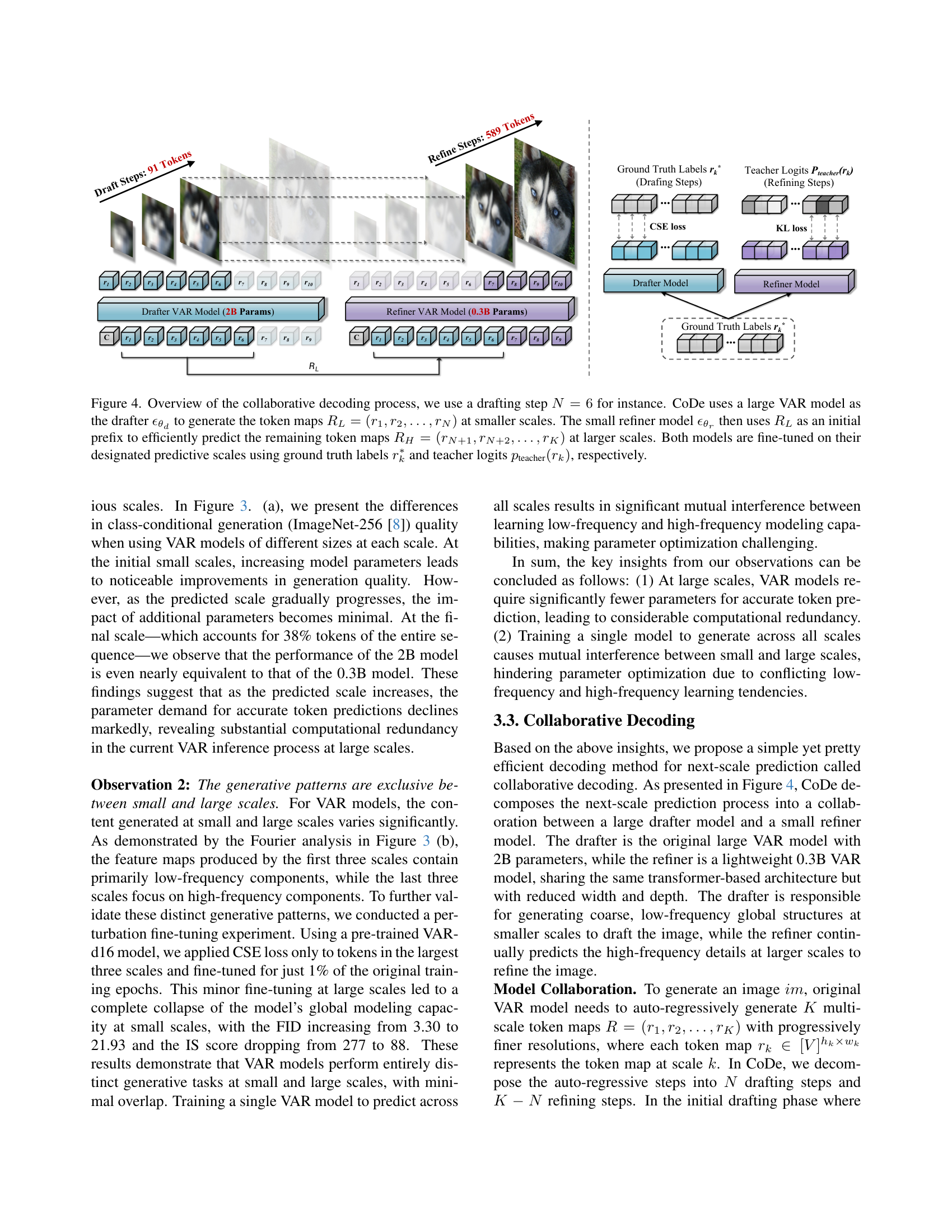
🔼 This figure illustrates the collaborative decoding process used in the proposed CoDe method. A large VAR model (the drafter) initially generates low-frequency token maps for smaller scales (up to scale N, where N=6 in this example). Then, a smaller VAR model (the refiner), using these token maps as a prefix, efficiently predicts the remaining high-frequency token maps for larger scales. Both models undergo fine-tuning using ground truth labels and teacher logits to optimize their performance at specific scales.
read the caption
Figure 4: Overview of the collaborative decoding process, we use a drafting step N=6𝑁6N=6italic_N = 6 for instance. CoDe uses a large VAR model as the drafter ϵθdsubscriptitalic-ϵsubscript𝜃𝑑\epsilon_{\theta_{d}}italic_ϵ start_POSTSUBSCRIPT italic_θ start_POSTSUBSCRIPT italic_d end_POSTSUBSCRIPT end_POSTSUBSCRIPT to generate the token maps RL=(r1,r2,…,rN)subscript𝑅𝐿subscript𝑟1subscript𝑟2…subscript𝑟𝑁R_{L}=(r_{1},r_{2},\ldots,r_{N})italic_R start_POSTSUBSCRIPT italic_L end_POSTSUBSCRIPT = ( italic_r start_POSTSUBSCRIPT 1 end_POSTSUBSCRIPT , italic_r start_POSTSUBSCRIPT 2 end_POSTSUBSCRIPT , … , italic_r start_POSTSUBSCRIPT italic_N end_POSTSUBSCRIPT ) at smaller scales. The small refiner model ϵθrsubscriptitalic-ϵsubscript𝜃𝑟\epsilon_{\theta_{r}}italic_ϵ start_POSTSUBSCRIPT italic_θ start_POSTSUBSCRIPT italic_r end_POSTSUBSCRIPT end_POSTSUBSCRIPT then uses RLsubscript𝑅𝐿R_{L}italic_R start_POSTSUBSCRIPT italic_L end_POSTSUBSCRIPT as an initial prefix to efficiently predict the remaining token maps RH=(rN+1,rN+2,…,rK)subscript𝑅𝐻subscript𝑟𝑁1subscript𝑟𝑁2…subscript𝑟𝐾R_{H}=(r_{N+1},r_{N+2},\ldots,r_{K})italic_R start_POSTSUBSCRIPT italic_H end_POSTSUBSCRIPT = ( italic_r start_POSTSUBSCRIPT italic_N + 1 end_POSTSUBSCRIPT , italic_r start_POSTSUBSCRIPT italic_N + 2 end_POSTSUBSCRIPT , … , italic_r start_POSTSUBSCRIPT italic_K end_POSTSUBSCRIPT ) at larger scales. Both models are fine-tuned on their designated predictive scales using ground truth labels rk∗superscriptsubscript𝑟𝑘r_{k}^{*}italic_r start_POSTSUBSCRIPT italic_k end_POSTSUBSCRIPT start_POSTSUPERSCRIPT ∗ end_POSTSUPERSCRIPT and teacher logits pteacher(rk)subscript𝑝teachersubscript𝑟𝑘p_{\text{teacher}}(r_{k})italic_p start_POSTSUBSCRIPT teacher end_POSTSUBSCRIPT ( italic_r start_POSTSUBSCRIPT italic_k end_POSTSUBSCRIPT ), respectively.

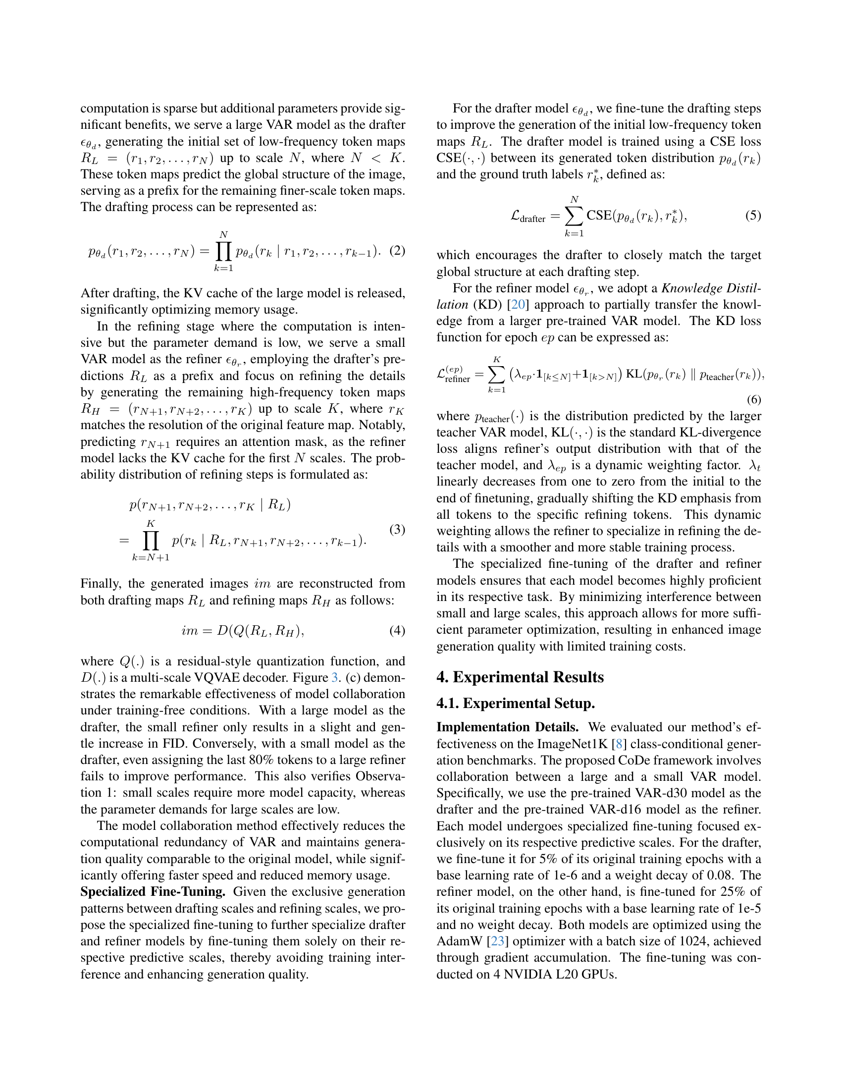
🔼 Figure 5 presents a comparison of different image generation methods, focusing on efficiency and quality. (a) shows that CoDe achieves the best balance between speed and FID score compared to other methods. (b) compares the inference latency of CoDe and VAR-d30 across different batch sizes, demonstrating CoDe’s efficiency. Finally, (c) shows that in the multi-scale decoding process of CoDe, the refiner model is more efficient at larger scales than the drafter model.
read the caption
Figure 5: (a) Our CoDe demonstrates the optimal efficiency-quality trade-off among all evaluated methods. (b) Inference latency is measured across varying batch sizes for the original VAR-d30, our CoDe (N=6), and the VQVAE decoder. (c) We analyze the time cost associated with parallel decoding at each scale, showing that the refiner model is significantly more efficient than the drafter at larger scales.
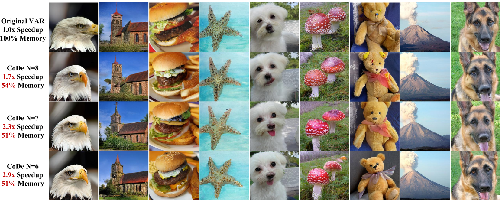
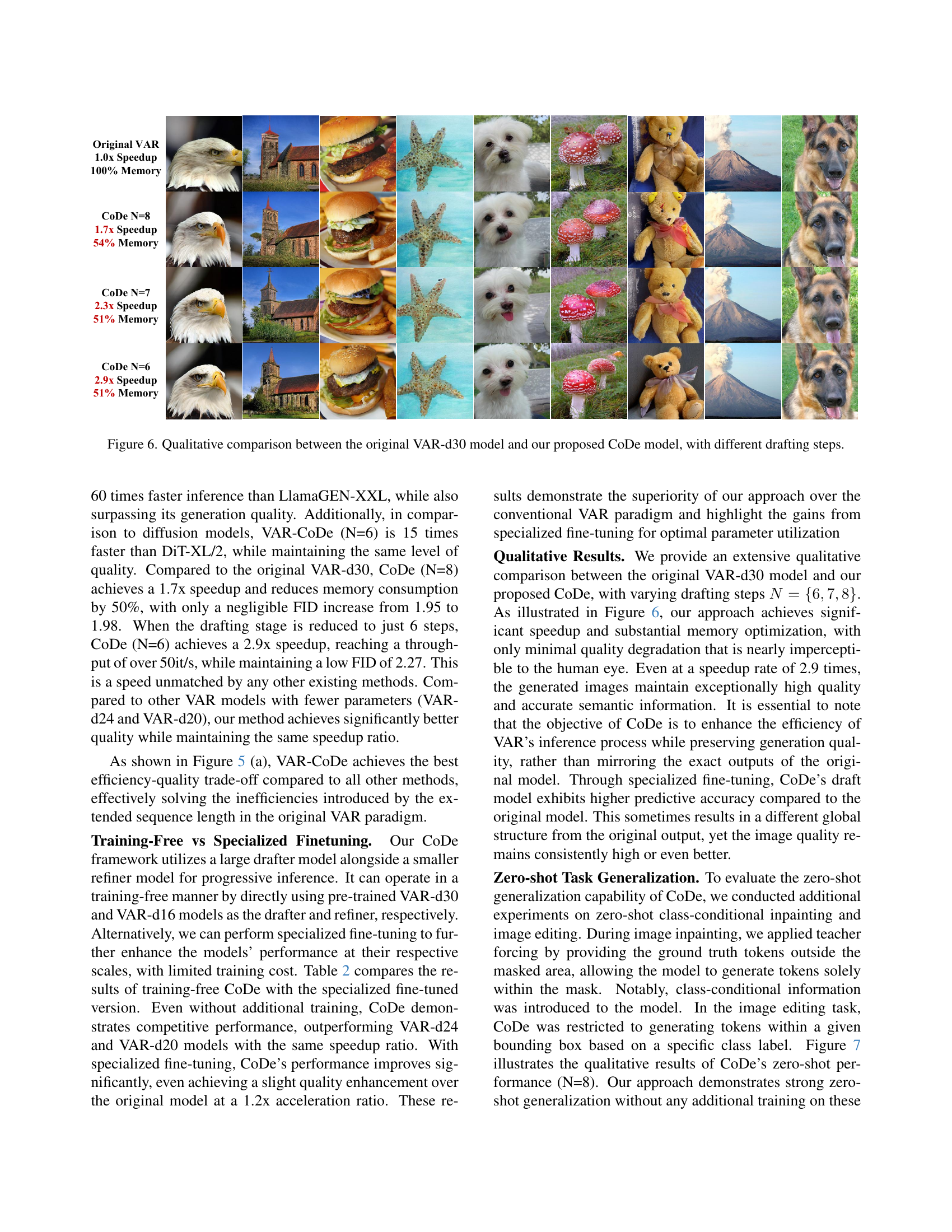
🔼 This figure displays a qualitative comparison of image generation results between the original VAR-d30 model and the proposed CoDe model with varying drafting steps (N=6, 7, 8). Each row shows generated images from a model, highlighting the speed and memory efficiency gains achieved by CoDe while maintaining comparable image quality. The original VAR-d30 serves as the baseline, illustrating the trade-off between speed and quality as the number of drafting steps decreases.
read the caption
Figure 6: Qualitative comparison between the original VAR-d30 model and our proposed CoDe model, with different drafting steps.
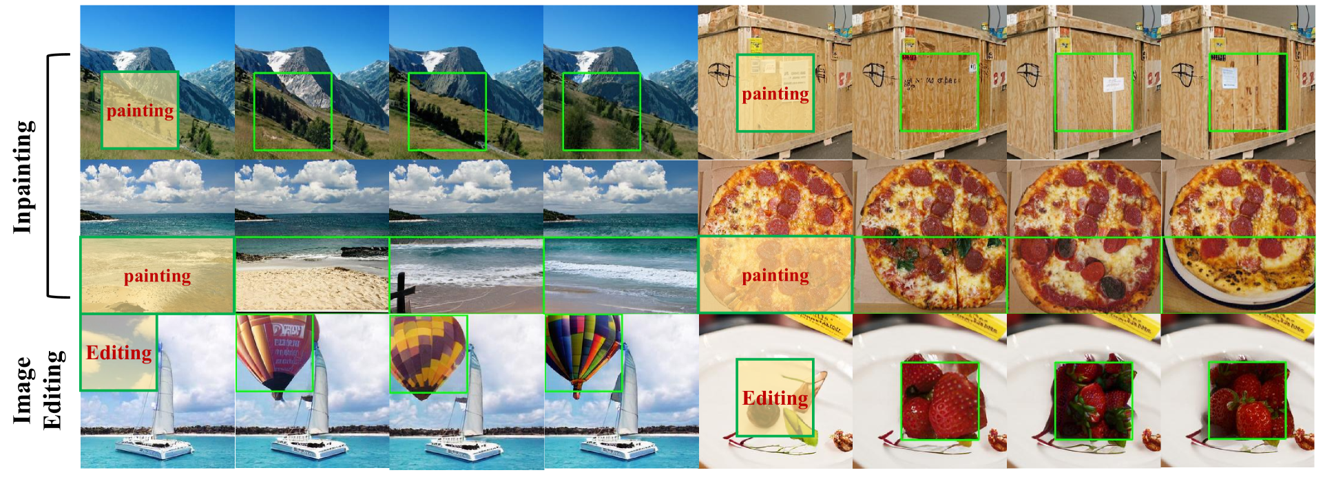
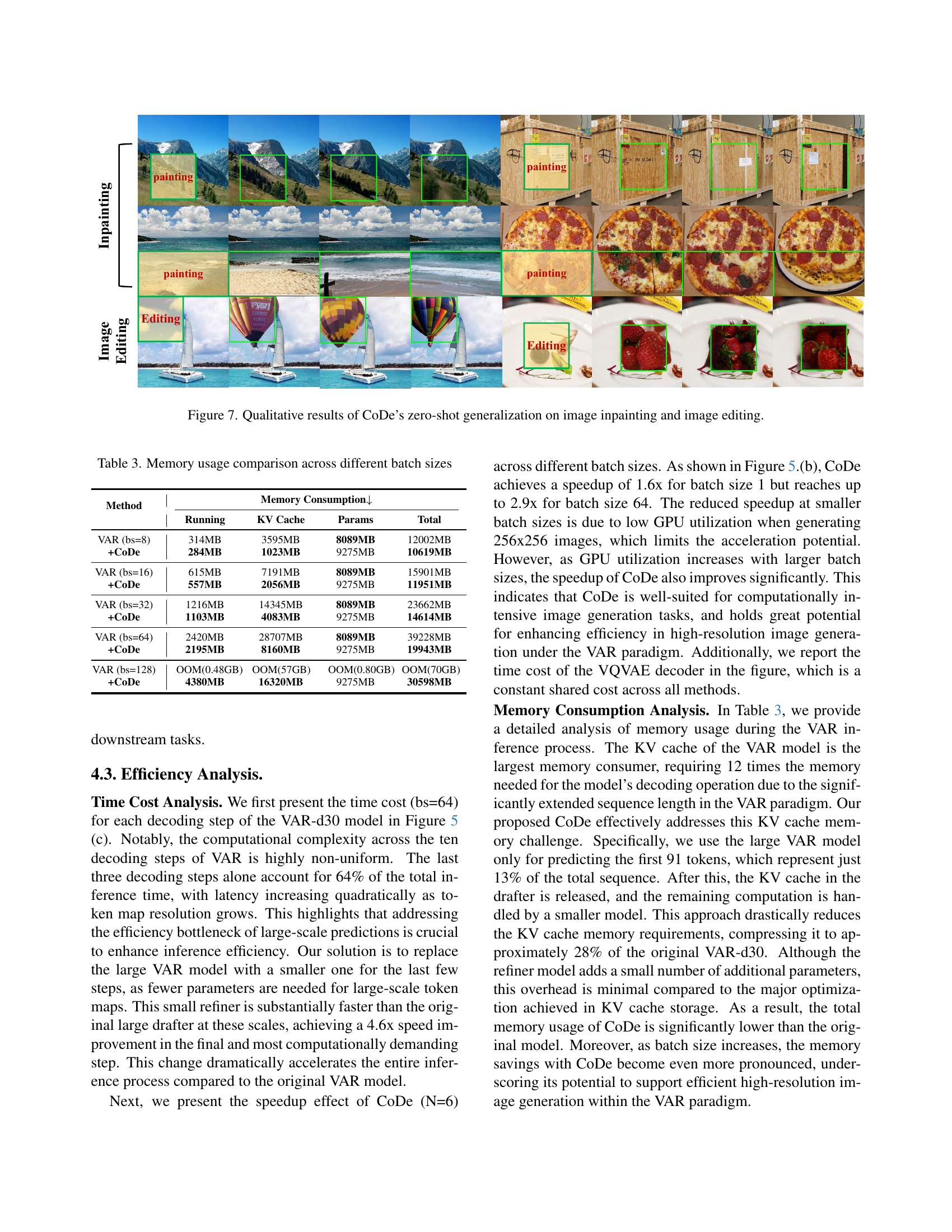
🔼 This figure showcases the zero-shot generalization capabilities of the Collaborative Decoding (CoDe) method on image inpainting and image editing tasks. The results demonstrate CoDe’s ability to perform these tasks without any additional training. The images presented illustrate examples of the inpainting and editing results achieved using CoDe.
read the caption
Figure 7: Qualitative results of CoDe’s zero-shot generalization on image inpainting and image editing.

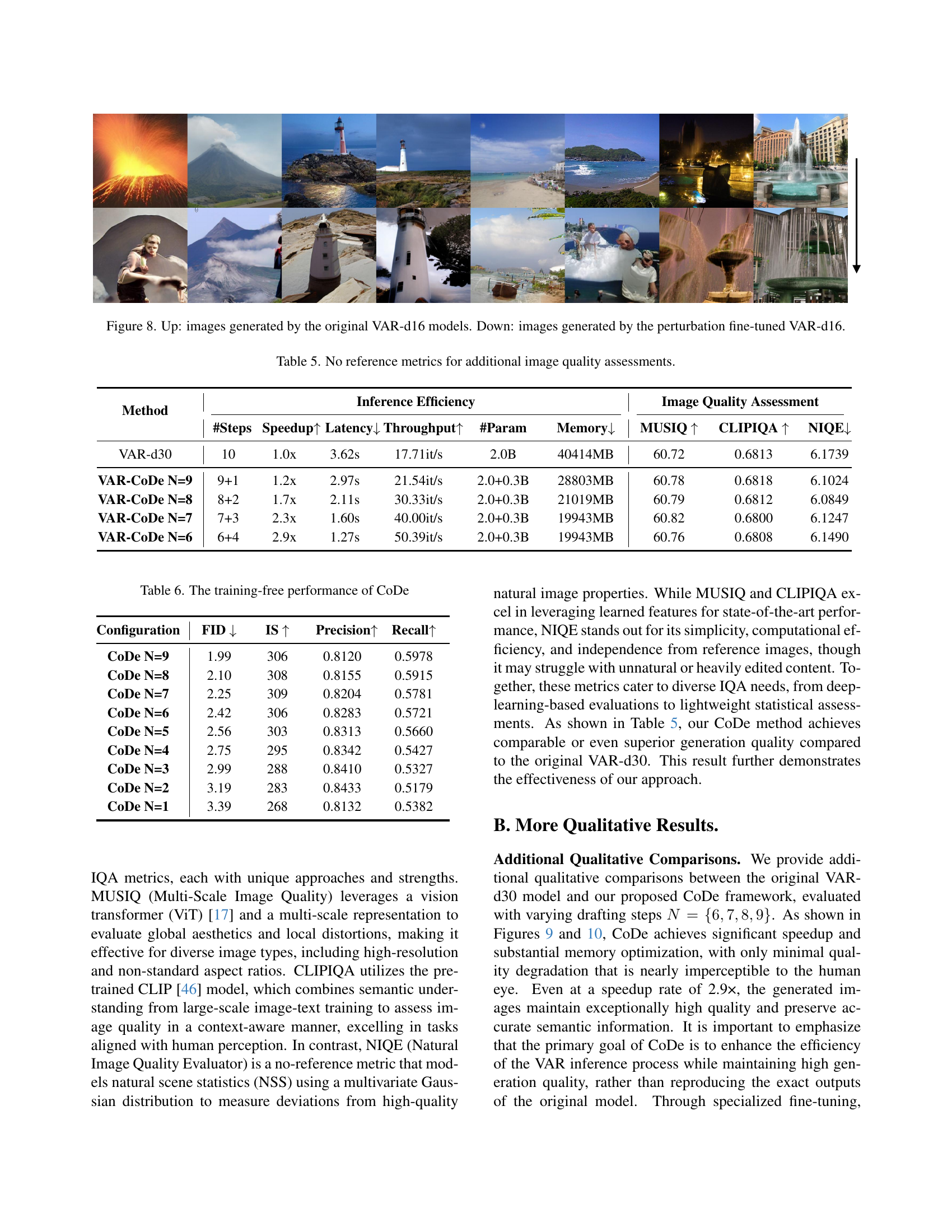
🔼 This figure shows a comparison of image generation results between the original VAR-d16 model and a version fine-tuned using a perturbation technique. The ‘Up’ section displays images generated by the standard VAR-d16 model, showcasing its typical output. The ‘Down’ section shows images generated after the model underwent perturbation fine-tuning, which selectively modifies the model’s parameters for higher-frequency components in the final scales, specifically focusing on details. By comparing the two sets of images, one can visually assess the impact of this perturbation method on the generated image quality and detail preservation.
read the caption
Figure 8: Up: images generated by the original VAR-d16 models. Down: images generated by the perturbation fine-tuned VAR-d16.

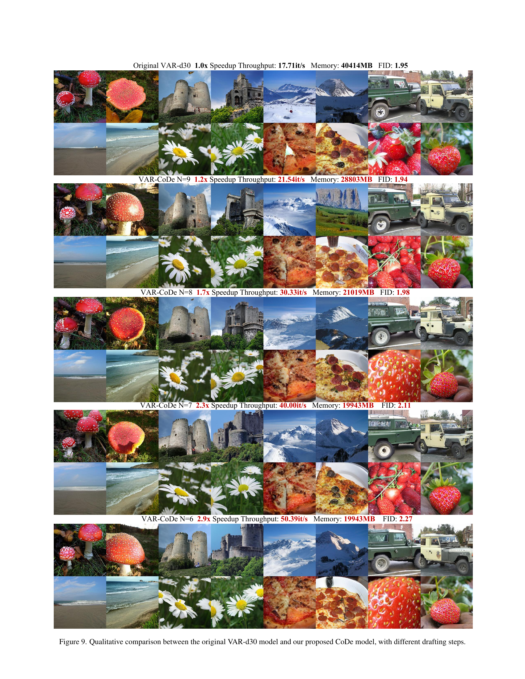
🔼 This figure presents a qualitative comparison of images generated by the original VAR-d30 model and the CoDe model with varying numbers of drafting steps (N=9, 8, 7, 6). Each row shows a set of generated images for the same set of prompts. The goal is to visually demonstrate how CoDe’s speed improvements (shown numerically in the caption) do not significantly impact image quality. The increasing speed is achieved by reducing the number of drafting steps and thereby reducing computational demands. A visual inspection allows assessing whether the speed improvements come at the cost of image quality.
read the caption
Figure 9: Qualitative comparison between the original VAR-d30 model and our proposed CoDe model, with different drafting steps.

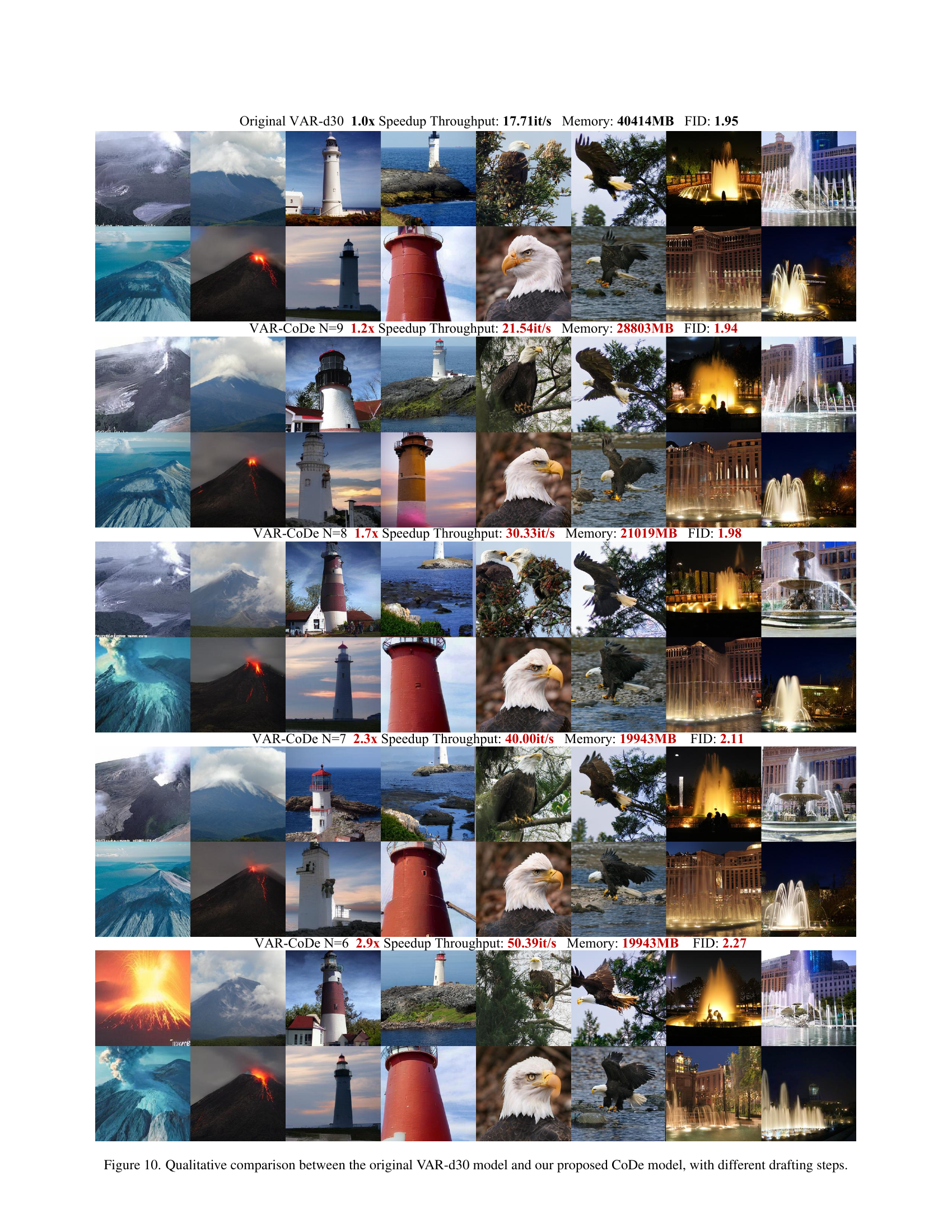
🔼 Figure 10 presents a qualitative comparison of image generation results between the original VAR-d30 model and the proposed CoDe model with varying numbers of drafting steps (N). Each row displays images generated using a different model (original VAR-d30 or CoDe with N=9, 8, 7, or 6). The figure visually demonstrates the impact of reducing the number of drafting steps on image quality while increasing speed and reducing memory usage. The FID (Fréchet Inception Distance) scores for each model are also provided, showing a small increase in FID (a measure of image quality) as the number of drafting steps decreases, and speedup factors are given.
read the caption
Figure 10: Qualitative comparison between the original VAR-d30 model and our proposed CoDe model, with different drafting steps.
More on tables
| Discription | N=6 | N=7 | N=8 | N=9 |
|---|---|---|---|---|
| CoDe Training-free | 2.42 | 2.26 | 2.10 | 1.99 |
| CoDe Fine-tuning | 2.27 | 2.11 | 1.98 | 1.94 |
🔼 This table shows the impact of specialized fine-tuning on the Collaborative Decoding (CoDe) method. It presents FID scores and speedup factors for different numbers of drafting steps (N) in the CoDe framework. The ‘Training-free’ row indicates the performance without any fine-tuning, showing the performance baseline. The other rows illustrate the improvements achieved through fine-tuning the model. This allows for a comparison of the performance trade-offs between training-free operation and the benefits of specialized fine-tuning.
read the caption
Table 2: Effect of specialized fine-tuning
| Method | Running | KV Cache | Params | Total |
|---|---|---|---|---|
| VAR (bs=8) | 314MB | 3595MB | 8089MB | 12002MB |
| +CoDe | 284MB | 1023MB | 9275MB | 10619MB |
| VAR (bs=16) | 615MB | 7191MB | 8089MB | 15901MB |
| +CoDe | 557MB | 2056MB | 9275MB | 11951MB |
| VAR (bs=32) | 1216MB | 14345MB | 8089MB | 23662MB |
| +CoDe | 1103MB | 4083MB | 9275MB | 14614MB |
| VAR (bs=64) | 2420MB | 28707MB | 8089MB | 39228MB |
| +CoDe | 2195MB | 8160MB | 9275MB | 19943MB |
| VAR (bs=128) | OOM(0.48GB) | OOM(57GB) | OOM(0.80GB) | OOM(70GB) |
| +CoDe | 4380MB | 16320MB | 9275MB | 30598MB |
🔼 This table compares the memory usage of the original VAR model and the proposed CoDe model across different batch sizes (8, 16, 32, 64, and 128). For each batch size, it breaks down the memory consumption into three categories: running memory (memory used during the model’s execution), KV cache (memory used for storing key-value pairs in the attention mechanism), and model parameters. The total memory usage is also shown. The table demonstrates how CoDe significantly reduces memory usage compared to the original VAR model, especially for larger batch sizes. Out of memory (OOM) errors occur for the original VAR at batch size 128, which are avoided by CoDe.
read the caption
Table 3: Memory usage comparison across different batch sizes
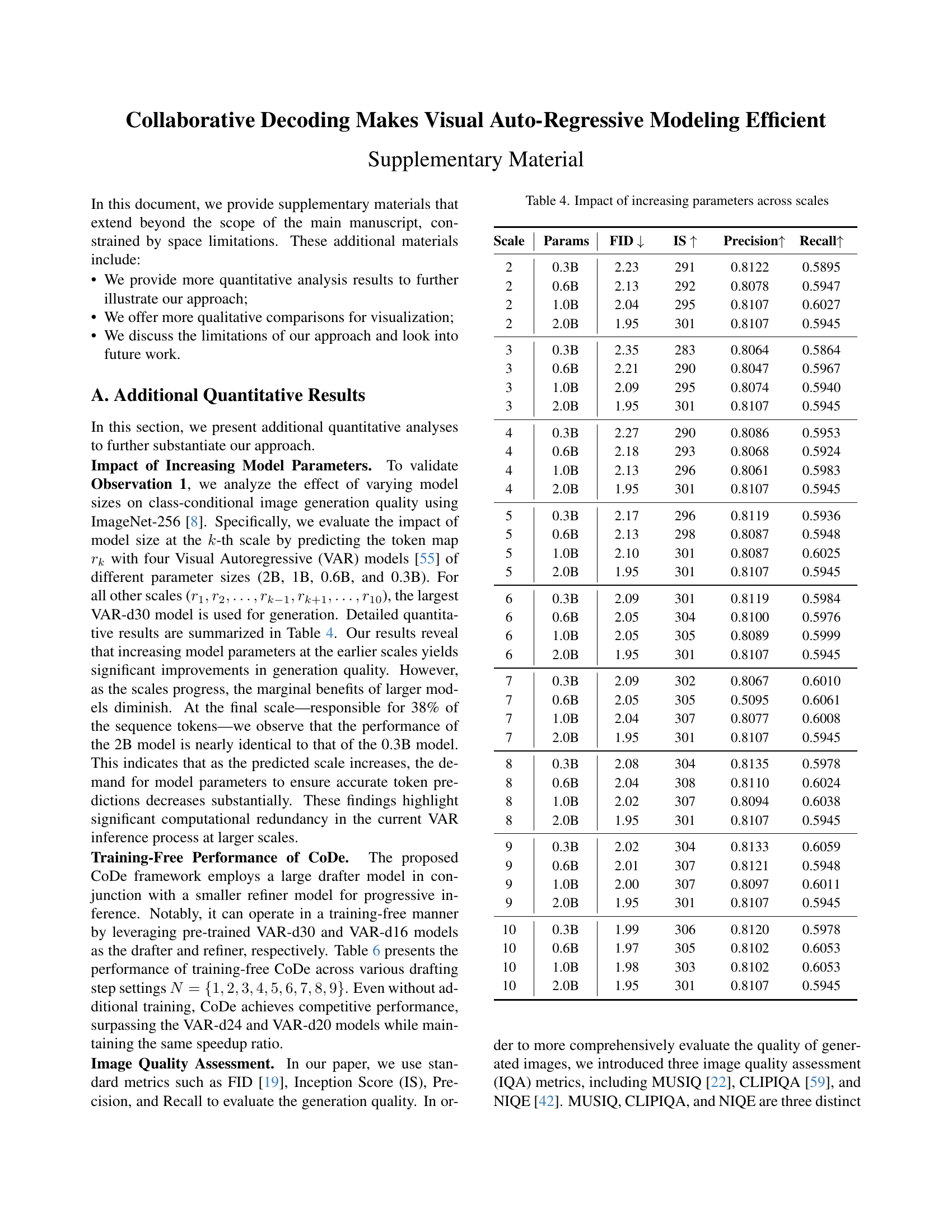
| Scale | Params | FID ↓ | IS ↑ | Precision ↑ | Recall ↑ |
|---|---|---|---|---|---|
| 2 | 0.3B | 2.23 | 291 | 0.8122 | 0.5895 |
| 2 | 0.6B | 2.13 | 292 | 0.8078 | 0.5947 |
| 2 | 1.0B | 2.04 | 295 | 0.8107 | 0.6027 |
| 2 | 2.0B | 1.95 | 301 | 0.8107 | 0.5945 |
| 3 | 0.3B | 2.35 | 283 | 0.8064 | 0.5864 |
| 3 | 0.6B | 2.21 | 290 | 0.8047 | 0.5967 |
| 3 | 1.0B | 2.09 | 295 | 0.8074 | 0.5940 |
| 3 | 2.0B | 1.95 | 301 | 0.8107 | 0.5945 |
| 4 | 0.3B | 2.27 | 290 | 0.8086 | 0.5953 |
| 4 | 0.6B | 2.18 | 293 | 0.8068 | 0.5924 |
| 4 | 1.0B | 2.13 | 296 | 0.8061 | 0.5983 |
| 4 | 2.0B | 1.95 | 301 | 0.8107 | 0.5945 |
| 5 | 0.3B | 2.17 | 296 | 0.8119 | 0.5936 |
| 5 | 0.6B | 2.13 | 298 | 0.8087 | 0.5948 |
| 5 | 1.0B | 2.10 | 301 | 0.8087 | 0.6025 |
| 5 | 2.0B | 1.95 | 301 | 0.8107 | 0.5945 |
| 6 | 0.3B | 2.09 | 301 | 0.8119 | 0.5984 |
| 6 | 0.6B | 2.05 | 304 | 0.8100 | 0.5976 |
| 6 | 1.0B | 2.05 | 305 | 0.8089 | 0.5999 |
| 6 | 2.0B | 1.95 | 301 | 0.8107 | 0.5945 |
| 7 | 0.3B | 2.09 | 302 | 0.8067 | 0.6010 |
| 7 | 0.6B | 2.05 | 305 | 0.5095 | 0.6061 |
| 7 | 1.0B | 2.04 | 307 | 0.8077 | 0.6008 |
| 7 | 2.0B | 1.95 | 301 | 0.8107 | 0.5945 |
| 8 | 0.3B | 2.08 | 304 | 0.8135 | 0.5978 |
| 8 | 0.6B | 2.04 | 308 | 0.8110 | 0.6024 |
| 8 | 1.0B | 2.02 | 307 | 0.8094 | 0.6038 |
| 8 | 2.0B | 1.95 | 301 | 0.8107 | 0.5945 |
| 9 | 0.3B | 2.02 | 304 | 0.8133 | 0.6059 |
| 9 | 0.6B | 2.01 | 307 | 0.8121 | 0.5948 |
| 9 | 1.0B | 2.00 | 307 | 0.8097 | 0.6011 |
| 9 | 2.0B | 1.95 | 301 | 0.8107 | 0.5945 |
| 10 | 0.3B | 1.99 | 306 | 0.8120 | 0.5978 |
| 10 | 0.6B | 1.97 | 305 | 0.8102 | 0.6053 |
| 10 | 1.0B | 1.98 | 303 | 0.8102 | 0.6053 |
| 10 | 2.0B | 1.95 | 301 | 0.8107 | 0.5945 |
🔼 This table shows the impact of increasing model parameters at different scales on image generation quality. The experiment predicts tokens for a single scale using models of varying sizes (0.3B, 0.6B, 1.0B, and 2.0B parameters), while using the largest model (2B) for all other scales. The results demonstrate that increasing parameters significantly improves quality at smaller scales, but this improvement diminishes as the scale increases; at the final scale, the largest model shows little advantage over the smallest.
read the caption
Table 4: Impact of increasing parameters across scales
| Method | #Steps | Speedup ↑ | Latency ↓ | Throughput ↑ | #Param | Memory ↓ | MUSIQ ↑ | CLIPIQA ↑ | NIQE ↓ |
|---|---|---|---|---|---|---|---|---|---|
| VAR-d30 | 10 | 1.0x | 3.62s | 17.71it/s | 2.0B | 40414MB | 60.72 | 0.6813 | 6.1739 |
| VAR-CoDe N=9 | 9+1 | 1.2x | 2.97s | 21.54it/s | 2.0+0.3B | 28803MB | 60.78 | 0.6818 | 6.1024 |
| VAR-CoDe N=8 | 8+2 | 1.7x | 2.11s | 30.33it/s | 2.0+0.3B | 21019MB | 60.79 | 0.6812 | 6.0849 |
| VAR-CoDe N=7 | 7+3 | 2.3x | 1.60s | 40.00it/s | 2.0+0.3B | 19943MB | 60.82 | 0.6800 | 6.1247 |
| VAR-CoDe N=6 | 6+4 | 2.9x | 1.27s | 50.39it/s | 2.0+0.3B | 19943MB | 60.76 | 0.6808 | 6.1490 |
🔼 This table presents a comparison of image quality metrics for different models. It assesses the performance of the original VAR-d30 model and several variants of CoDe (Collaborative Decoding) with varying numbers of drafting steps (N). The metrics used are not reference-based (meaning they don’t compare to a ground truth image), instead relying on metrics that evaluate the image quality itself. The metrics included are MUSIQ, CLIPIQA, and NIQE, each offering a different perspective on image quality, providing a more comprehensive assessment than FID and IS alone. The table shows how different models trade off efficiency (speedup, throughput) with various image quality aspects.
read the caption
Table 5: No reference metrics for additional image quality assessments.
| Configuration | FID ↓ | IS ↑ | Precision ↑ | Recall ↑ |
|---|---|---|---|---|
| CoDe N=9 | 1.99 | 306 | 0.8120 | 0.5978 |
| CoDe N=8 | 2.10 | 308 | 0.8155 | 0.5915 |
| CoDe N=7 | 2.25 | 309 | 0.8204 | 0.5781 |
| CoDe N=6 | 2.42 | 306 | 0.8283 | 0.5721 |
| CoDe N=5 | 2.56 | 303 | 0.8313 | 0.5660 |
| CoDe N=4 | 2.75 | 295 | 0.8342 | 0.5427 |
| CoDe N=3 | 2.99 | 288 | 0.8410 | 0.5327 |
| CoDe N=2 | 3.19 | 283 | 0.8433 | 0.5179 |
| CoDe N=1 | 3.39 | 268 | 0.8132 | 0.5382 |
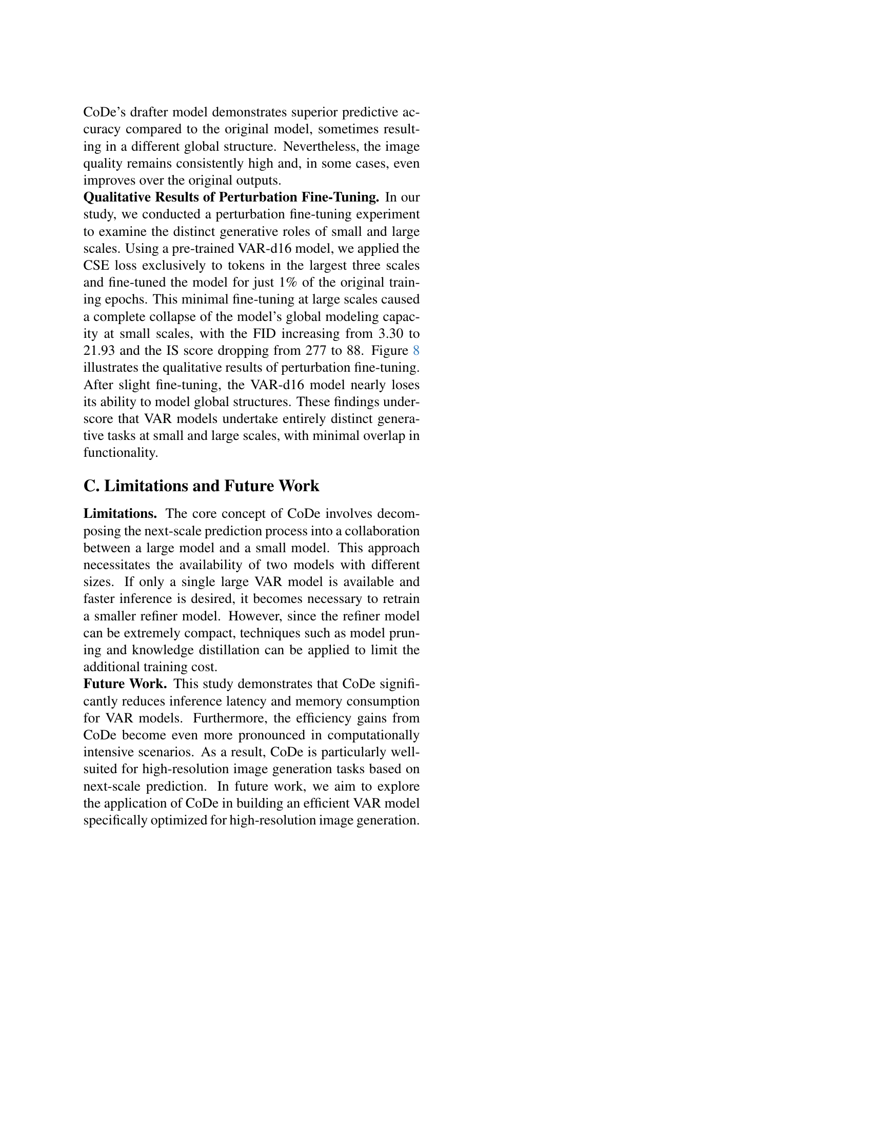
🔼 This table presents the performance of the Collaborative Decoding (CoDe) method without any additional training. It shows the FID (Fréchet Inception Distance), Inception Score (IS), Precision, and Recall metrics for different numbers of drafting steps (N) in CoDe. Lower FID scores indicate better image quality. Higher IS, precision, and recall values suggest improved image generation performance.
read the caption
Table 6: The training-free performance of CoDe
Full paper#
