↗ arXiv ↗ Hugging Face ↗ Papers with Code
TL;DR#
Large language models (LLMs) rely heavily on induction heads for their in-context learning capabilities. However, implementing efficient induction heads requires significant computational resources, often necessitating deep and wide transformer architectures. This paper tackles this challenge by introducing a new method called KV shifting attention.
KV shifting attention elegantly simplifies the induction process by decoupling keys and values in the attention mechanism. This innovative approach significantly reduces the depth and width requirements for induction heads, enabling even single-layer transformers to perform induction tasks effectively. The researchers demonstrate the effectiveness of their method through theoretical analysis and empirical evaluation on various models. Their findings indicate that KV shifting attention achieves comparable or superior performance to multi-layer transformers, offering a more efficient and faster training process for LLMs.
Key Takeaways#
Why does it matter?#
This paper is important because it introduces a novel attention mechanism, KV shifting attention, that improves language modeling by reducing the computational demands of induction heads. This has significant implications for the development of more efficient and effective large language models. It provides theoretical analysis, experimental validation, and opens up new avenues for research in transformer architecture optimization. The findings are relevant to current trends in efficient and effective LLMs, especially with implications for resource constrained settings.
Visual Insights#

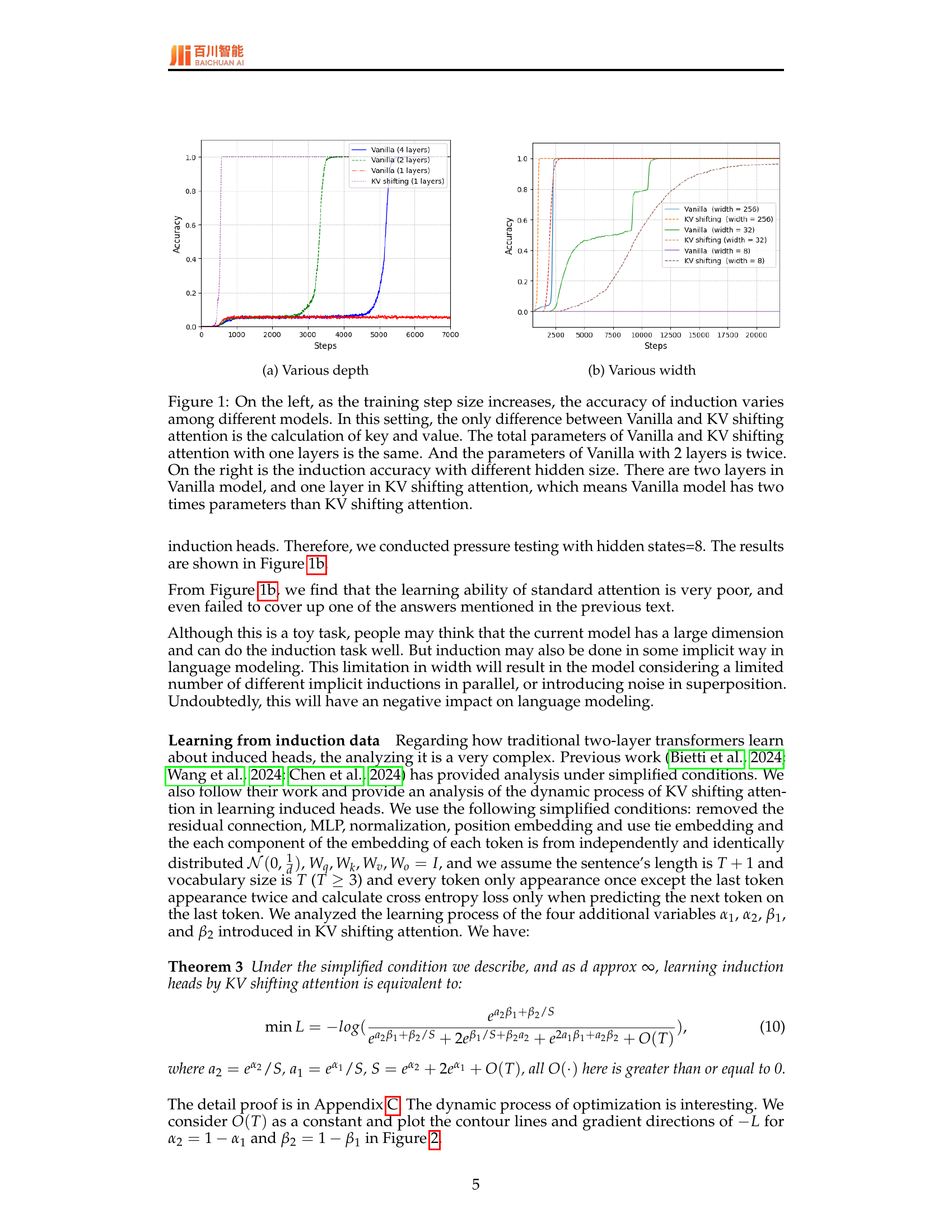
🔼 The figure shows how the accuracy of induction varies among different models with different depths (number of layers). The training step size is the only parameter that changes. The KV shifting attention (1-layer) achieves comparable performance to the vanilla model with 2 layers, and both significantly outperform the vanilla model with only 1 layer, demonstrating the effectiveness of KV shifting attention in reducing the depth requirement for induction head learning.
read the caption
(a) Various depth
| Parameters | 1.5B | 2.9B | 6.7B | 13B | 19B |
|---|---|---|---|---|---|
| Hidden size | 2,048 | 2,560 | 4,096 | 5,120 | 6,144 |
| Layers | 28 | 32 | 32 | 40 | 48 |
| Head Number | 16 | 20 | 32 | 40 | 48 |
| KV Number | 16 | 4 | 32 | 40 | 4 |
| FFN size | 5,504 | 8,704 | 11,008 | 13,824 | 16,384 |
| Max Length | 2,048 | 4,096 | 2,048 | 2,048 | 12,288 |
| Total Tokens | 10B | 500B | 10B | 10B | 200B |
| Vocab size | 36,000 | 48,000 | 36,000 | 36,000 | 48,000 |
🔼 This table details the architecture and hyperparameters of the language models used in the experiments. It shows the different sizes of the models (1.5B, 2.9B, 6.7B, 13B, and 19B parameters), their key architectural components (hidden size, number of layers, number of heads, and feed-forward network size), and training parameters (maximum sequence length, vocabulary size, and other relevant training settings).
read the caption
Table 1: Model Configuration.
In-depth insights#
KV Shifting Attention#
The proposed “KV Shifting Attention” mechanism offers a novel approach to enhancing language models by modifying the attention mechanism. Instead of the standard approach where query, key, and value vectors are independently computed, this method decouples keys and values, enabling a more flexible and efficient induction process. This decoupling is achieved by shifting the key and value vectors relative to the query vector, allowing the model to capture information from surrounding tokens more effectively. This is particularly beneficial for learning induction heads, which are essential components in a language model’s capacity for in-context learning, reducing the need for deeper and wider transformer architectures. The theoretical analysis demonstrates how KV Shifting Attention reduces the depth and width requirements for effective induction head learning, leading to more efficient model training and improved performance, even in large-scale pre-trained models. Experimental results further support the efficacy of this approach, showing comparable or superior performance compared to conventional multi-layer transformers across diverse model sizes. The inherent bias towards learning induction heads contributes to more efficient and effective language modeling.
Induction Head Analysis#
An in-depth analysis of induction heads in transformer-based language models would explore their crucial role in in-context learning (ICL). It would delve into the mechanisms by which induction heads identify and leverage repeating patterns within input sequences, enabling the model to perform tasks like multi-step reasoning and complex inference. The analysis should investigate the structural requirements of induction heads, including depth (number of layers) and width (number of attention heads), and discuss the trade-offs between these factors and model performance. A critical part of the analysis would involve studying the learning dynamics of induction heads, examining how they acquire and represent inductive knowledge during training. This would include analyzing the influence of various architectural choices and training strategies on the effectiveness of induction head learning. Finally, a comprehensive analysis would assess the limitations of current induction head mechanisms, exploring their potential failure modes and areas for future research, for instance, how their performance is affected by input sequence length and complexity.
Model Scaling Effects#
Model scaling effects in large language models (LLMs) are a complex interplay of various factors. Increasing model size (parameters) generally leads to improved performance on a wide range of tasks, a phenomenon often described by scaling laws. However, this improvement isn’t linear, and diminishing returns are observed beyond certain scales. Computational costs increase dramatically with model size, posing significant challenges. Furthermore, data requirements also scale, necessitating massive datasets for effective training of larger models. Beyond raw size, architectural choices and training techniques influence scaling behavior. Efficient architectures mitigate computational costs, while innovative training methods (e.g., Mixture of Experts) enhance scalability. Generalization ability is another key consideration; larger models often exhibit better generalization, but this depends on data quality and diversity. Therefore, studying model scaling effects requires a nuanced understanding of the trade-offs between performance gains, computational resources, data needs, architecture, and generalization capabilities. Optimal scaling strategies involve carefully considering these factors to achieve the desired balance of performance and efficiency.
Empirical Validation#
An Empirical Validation section in a research paper would rigorously test the proposed KV Shifting Attention mechanism. This would involve designing experiments to compare its performance against existing methods across various aspects. Key metrics would include accuracy on language modeling benchmarks (like GLUE or SuperGLUE), training speed, and parameter efficiency. Different model sizes (small, medium, large) should be tested. The choice of datasets is crucial; experiments should cover diverse domains and styles to check for robustness. Control experiments are needed to isolate the impact of KV Shifting, for instance, comparing it to standard multi-layer transformers with similar complexity. Results should be presented with statistical significance and error bars to highlight any reliable improvements. Qualitative analysis can add additional insights by analyzing attention patterns in the KV Shifting model to see if it learns induction heads more effectively. Finally, limitations of the empirical study should be clearly stated, for example, potential biases in data selection or constraints in computational resources. Thorough validation establishes confidence in the proposed method’s practical value.
Future Research#
Future research directions stemming from this paper on KV shifting attention for enhanced language modeling could explore several promising avenues. One key area is a deeper investigation into the theoretical underpinnings of KV shifting, potentially leading to a more rigorous mathematical framework for understanding its effectiveness. This could involve extending the analysis beyond the toy models and focusing on the behavior in large-scale language models. Furthermore, research should delve into the interaction between KV shifting and other architectural components, such as different attention mechanisms, normalization layers, or positional encodings. This would provide a more comprehensive understanding of how KV shifting affects overall model performance. Another significant area for future work involves evaluating the generalizability of KV shifting to diverse language modeling tasks beyond those explored in the paper. This includes testing its efficacy in multilingual, cross-lingual, and low-resource settings. Finally, exploring the interplay between KV shifting and the training process itself warrants further study. For instance, research could investigate optimal hyperparameter settings and training schedules tailored to KV-shifted models and analyze the impact on convergence speed and generalization. These future research directions would solidify the understanding of KV shifting and pave the way for more impactful advances in language modeling.
More visual insights#
More on figures

🔼 The figure shows how the accuracy of induction varies with different hidden sizes. There are two layers in the vanilla model and one layer in the KV shifting attention model; therefore, the vanilla model has twice the number of parameters. The results demonstrate that KV shifting attention achieves comparable accuracy to the two-layer vanilla model, even with a smaller width (fewer parameters), highlighting its efficiency in learning induction heads.
read the caption
(b) Various width

🔼 This figure compares the performance of standard multi-layer transformers (Vanilla) and the proposed KV shifting attention mechanism in learning induction heads. The left panel shows how accuracy in an induction task changes as the training progresses for one-layer and two-layer Vanilla models, and a one-layer KV shifting model. Note that the one-layer KV shifting model has the same number of parameters as the one-layer Vanilla model, while the two-layer Vanilla model has twice as many parameters. The right panel shows accuracy as a function of the hidden layer size. Again, the one-layer KV shifting model is compared to one-layer and two-layer Vanilla models. The results demonstrate that KV shifting attention improves induction learning, even when comparing models with the same number of parameters.
read the caption
Figure 1: On the left, as the training step size increases, the accuracy of induction varies among different models. In this setting, the only difference between Vanilla and KV shifting attention is the calculation of key and value. The total parameters of Vanilla and KV shifting attention with one layers is the same. And the parameters of Vanilla with 2 layers is twice. On the right is the induction accuracy with different hidden size. There are two layers in Vanilla model, and one layer in KV shifting attention, which means Vanilla model has two times parameters than KV shifting attention.

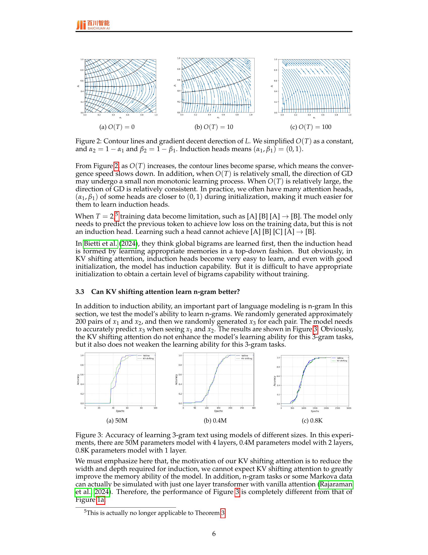
🔼 This figure shows contour lines and gradient descent directions of the loss function L for a simplified model used to analyze induction heads. The loss function is simplified by treating O(T) as a constant and setting α2 = 1 - α1 and β2 = 1 - β1. The plot shows how the contour lines and gradient directions change as O(T) increases from 0 to 10 to 100. When O(T) is small, the gradient descent is non-monotonic, but as O(T) increases, it becomes more consistent and it becomes easier for the model to learn induction heads as indicated by the gradient moving toward the point (α1, β1) = (0,1), representing an ideal induction head.
read the caption
(a) O(T)=0𝑂𝑇0O(T)=0italic_O ( italic_T ) = 0

🔼 This figure visualizes the contour lines and gradient descent direction of the loss function L in relation to the variables α₁ and β₁. The loss function represents the optimization objective during the training of the KV shifting attention mechanism. The contour lines show the level sets of the loss function, where points on the same line have the same loss value. The gradient descent vectors indicate the direction of steepest descent, which guides the training process to minimize the loss function. The parameter O(T) reflects the complexity of the task and controls how sparse the contour lines are (more sparse for larger O(T)). The figure shows three cases (O(T) = 0, O(T) = 10, O(T) = 100) with different densities of contour lines, illustrating the effect of task complexity on the optimization landscape.
read the caption
(b) O(T)=10𝑂𝑇10O(T)=10italic_O ( italic_T ) = 10

🔼 This figure shows contour lines and gradient descent directions for the loss function L when O(T) is set to 100. The contour lines represent the values of L, and the arrows indicate the direction of gradient descent. The gradient descent is an optimization process used to find the minimum value of the loss function. The sparseness of the contour lines indicates a slower convergence speed of the optimization algorithm. This visualization is used to illustrate the impact of the O(T) term on the model’s ability to learn induction heads.
read the caption
(c) O(T)=100𝑂𝑇100O(T)=100italic_O ( italic_T ) = 100

🔼 This figure visualizes the contour lines and gradient descent directions of the loss function (L) involved in learning induction heads using KV shifting attention. The analysis simplifies the complex loss function by treating O(T) (a term related to sequence length) as a constant. The plot focuses on the relationship between two learnable parameters, α1 and β1, while α2 and β2 are defined as 1-α1 and 1-β1 respectively. The point (α1, β1) = (0, 1) represents the ideal state of learning perfect induction heads. The contour lines show how quickly the loss function changes with respect to these parameters. The gradient descent directions indicate the direction the parameters are likely to move during training in order to minimize the loss, thus illustrating how effectively the KV shifting attention method facilitates the training process towards the ideal (0,1) state. Different subplots show the effect of varying the complexity of the training data, represented by O(T).
read the caption
Figure 2: Contour lines and gradient decent derection of L𝐿Litalic_L. We simplified O(T)𝑂𝑇O(T)italic_O ( italic_T ) as a constant, and α2=1−α1subscript𝛼21subscript𝛼1\alpha_{2}=1-\alpha_{1}italic_α start_POSTSUBSCRIPT 2 end_POSTSUBSCRIPT = 1 - italic_α start_POSTSUBSCRIPT 1 end_POSTSUBSCRIPT and β2=1−β1subscript𝛽21subscript𝛽1\beta_{2}=1-\beta_{1}italic_β start_POSTSUBSCRIPT 2 end_POSTSUBSCRIPT = 1 - italic_β start_POSTSUBSCRIPT 1 end_POSTSUBSCRIPT. Induction heads means (α1,β1)=(0,1)subscript𝛼1subscript𝛽101(\alpha_{1},\beta_{1})=(0,1)( italic_α start_POSTSUBSCRIPT 1 end_POSTSUBSCRIPT , italic_β start_POSTSUBSCRIPT 1 end_POSTSUBSCRIPT ) = ( 0 , 1 ).

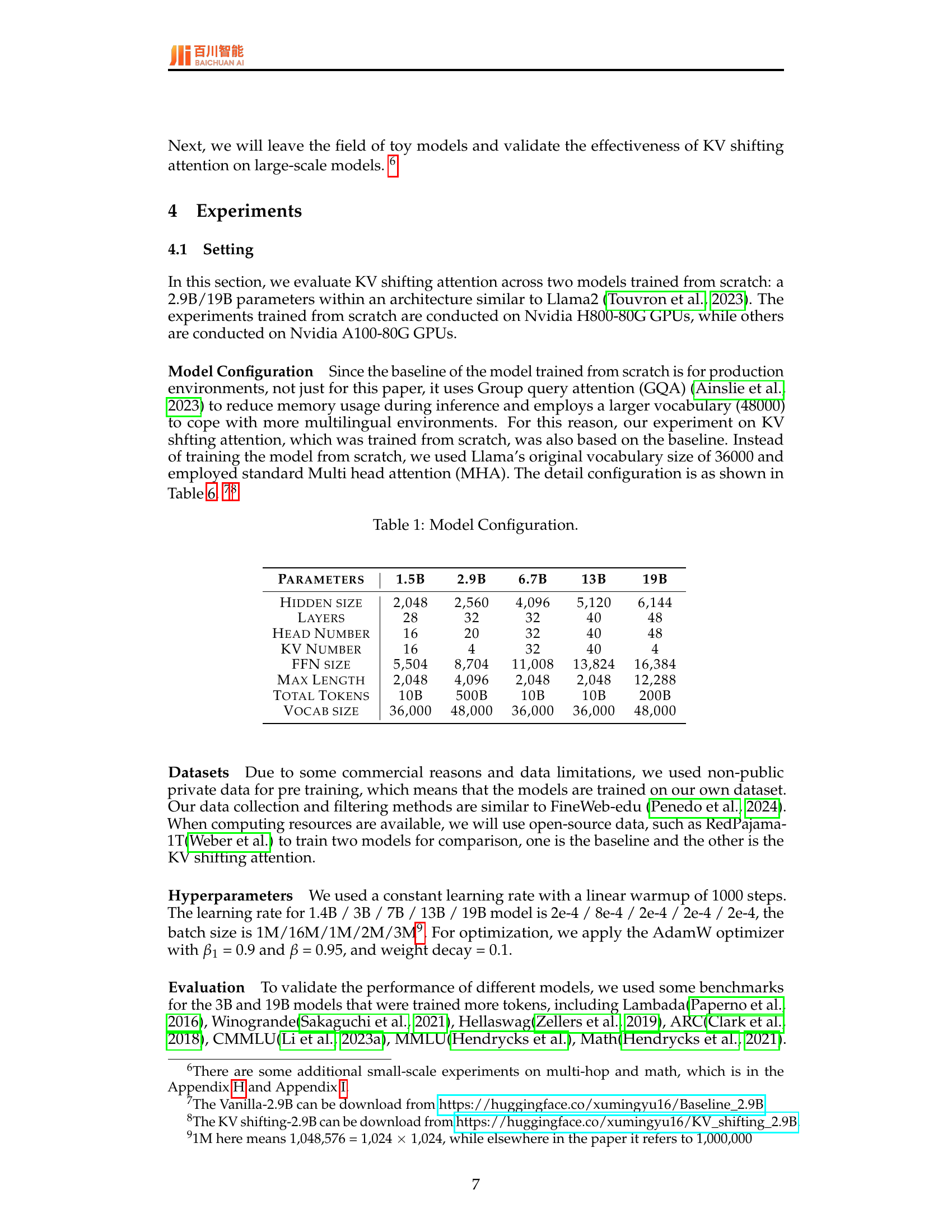
🔼 This figure shows the accuracy of learning 3-gram text using models of different sizes. The experiment includes three models: a 50M parameter model with 4 layers, a 0.4M parameter model with 2 layers, and a 0.8K parameter model with 1 layer. The x-axis represents the number of training epochs, and the y-axis represents the accuracy of predicting the third token in a sequence given the first two tokens. The purpose is to compare the performance of standard transformers (Vanilla) against KV shifting attention in learning n-grams. The results show that KV shifting attention does not significantly improve or hinder the ability to learn 3-grams compared to standard transformers across different model sizes.
read the caption
(a) 50M

🔼 This figure displays the accuracy of induction head learning across different model sizes and training steps. The experiment uses a simplified setting, focusing only on the ability to learn induction heads. The smaller model (0.4M parameters) is compared to a larger model (50M parameters), showing the influence of model size on induction head learning ability, measured by the accuracy of predicting subsequent tokens given a repeating pattern of preceding tokens. The graph demonstrates how well each model learns to identify and utilize these repeating patterns to make accurate predictions. The x-axis represents the number of training steps, while the y-axis indicates the accuracy of the induction head mechanism.
read the caption
(b) 0.4M

🔼 This figure shows the accuracy of learning 3-gram text using a model with 0.8K parameters. It compares the performance of a standard transformer (Vanilla) against the KV shifting attention model. The x-axis represents the training epochs, and the y-axis represents the accuracy. This experiment is designed to evaluate the models’ ability to learn n-grams, a fundamental aspect of language modeling. The results show how the accuracy of learning 3-grams changes over time for both models.
read the caption
(c) 0.8K

🔼 This figure compares the accuracy of learning 3-gram text across models with varying numbers of parameters and layers. The experiment demonstrates that even a single-layer model with a small number of parameters (0.8K) can achieve a relatively high accuracy. A model with 0.4M parameters and 2 layers performs better, and the largest model with 50M parameters and 4 layers achieves the highest accuracy. This highlights that more parameters and layers generally improve performance for this specific task. However, the single-layer model’s performance is still noteworthy given its parameter efficiency.
read the caption
Figure 3: Accuracy of learning 3-gram text using models of different sizes. In this experiments, there are 50M parameters model with 4 layers, 0.4M parameters model with 2 layers, 0.8K parameters model with 1 layer.

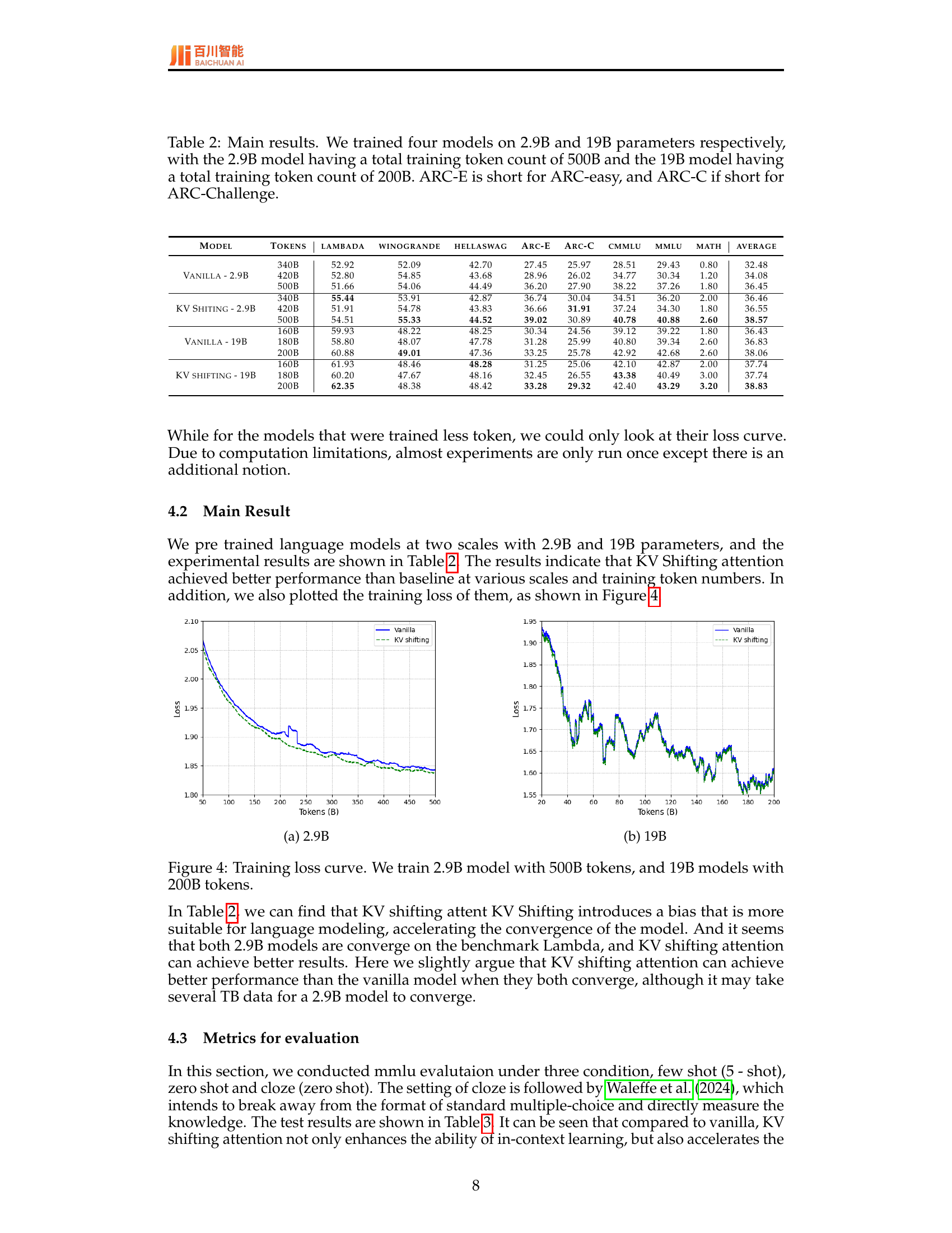
🔼 The training loss curves for the 2.9B parameter model are plotted, comparing the vanilla model with KV shifting attention. The x-axis represents the number of training tokens (in billions), and the y-axis shows the training loss. The plot illustrates the convergence speed and overall loss values of both models during training, highlighting the difference in their performance.
read the caption
(a) 2.9B

🔼 The figure shows the training loss curve for the 19B parameter model. The model was trained using 200B tokens. The blue line represents the training loss for the vanilla model, while the orange line represents the training loss for the model using KV shifting attention. The graph indicates that the model with KV shifting attention converges faster and achieves a lower final loss compared to the vanilla model. This demonstrates the efficacy of KV shifting attention in enhancing training efficiency and improving model performance.
read the caption
(b) 19B

🔼 This figure displays the training loss curves for two large language models: one with 2.9 billion parameters trained on 500 billion tokens and another with 19 billion parameters trained on 200 billion tokens. The curves show the decrease in training loss over the course of training, illustrating the models’ learning progress. Comparing the two curves allows for assessing the impact of model size and training data volume on the learning process.
read the caption
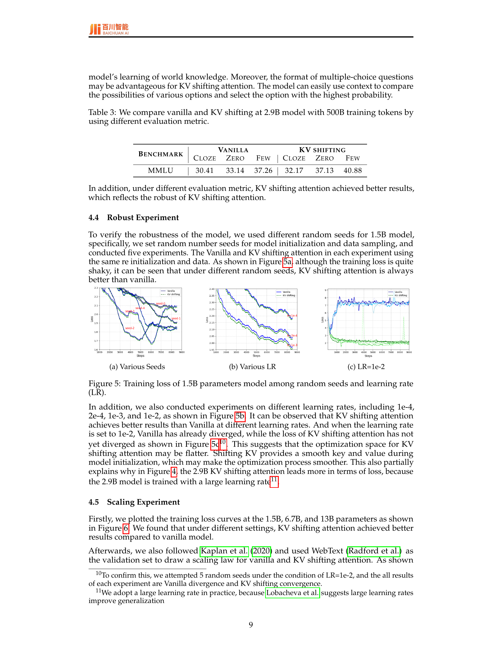
Figure 4: Training loss curve. We train 2.9B model with 500B tokens, and 19B models with 200B tokens.

🔼 This figure displays the training loss curves for a 1.5B parameter model across five different random seeds. Each curve represents a separate training run with different random initialization and data sampling. The purpose is to demonstrate the robustness of KV shifting attention compared to vanilla attention, showing that KV shifting attention consistently achieves lower training loss even under varied conditions.
read the caption
(a) Various Seeds
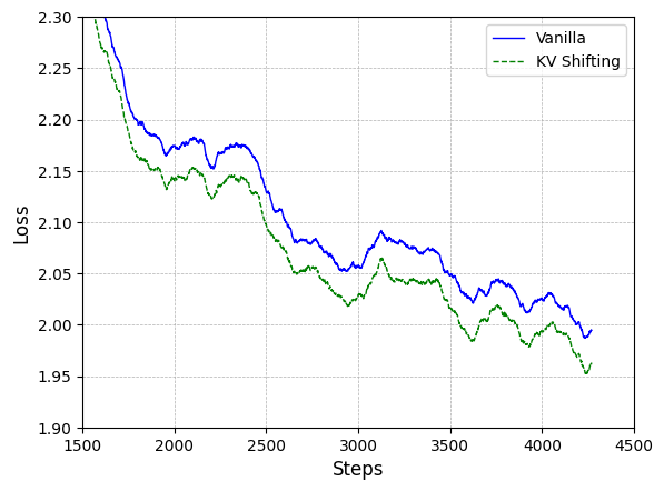
🔼 This figure shows the training loss curves for a 1.5B parameter model with different learning rates (LR). It compares the performance of the vanilla attention mechanism against the KV shifting attention mechanism across various learning rates. The goal is to assess the robustness and stability of each approach under different optimization settings, demonstrating how the KV shifting attention mechanism generally maintains stability even when the vanilla attention mechanism diverges (e.g., at LR=1e-2).
read the caption
(b) Various LR

🔼 This figure displays the training loss curves for a 1.5B parameter model using different learning rates. Specifically, it shows the impact of a 1e-2 learning rate on the training loss of both Vanilla attention and KV shifting attention. Note that the y-axis represents training loss and x-axis represents training steps. The plot helps illustrate the robustness and stability of KV shifting attention, particularly its resilience to higher learning rates, as compared to the Vanilla attention mechanism.
read the caption
(c) LR=1e-2
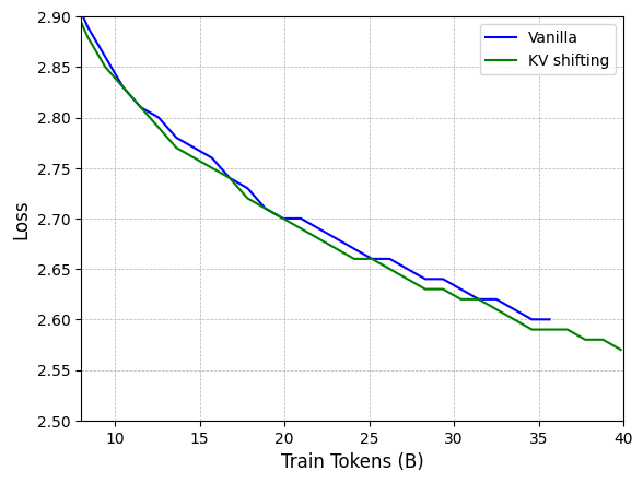
🔼 This figure displays the training loss curves for a 1.5B parameter language model under various conditions. Specifically, it illustrates how the training loss changes with the number of training steps across multiple runs using different random seeds for model initialization, and also shows how the loss varies when using different learning rates (LR). This allows for an assessment of the model’s robustness and stability during training across different random initializations and hyperparameter settings. The different lines represent separate training runs with different random seeds or learning rates.
read the caption
Figure 5: Training loss of 1.5B parameters model among random seeds and learning rate (LR).

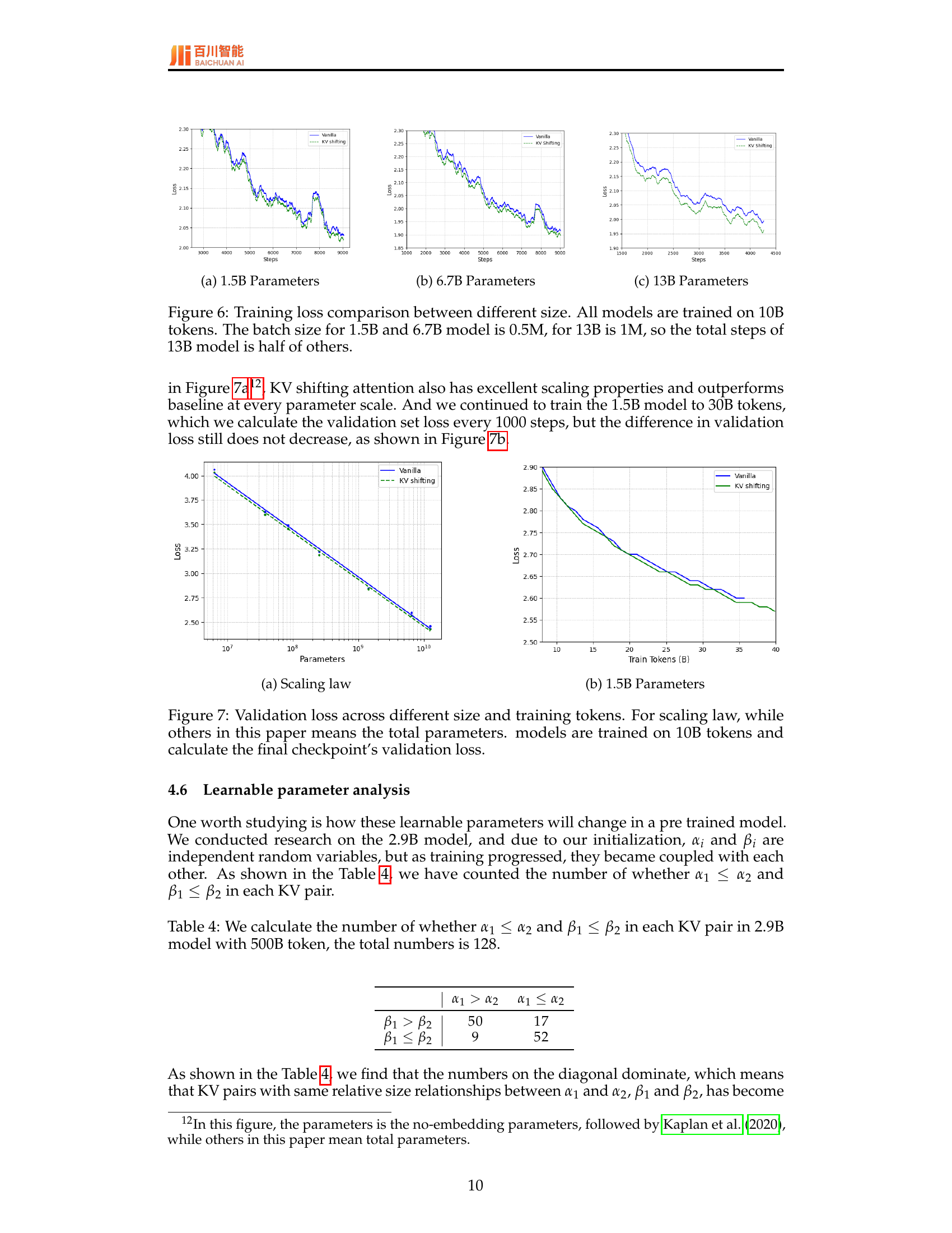
🔼 Training loss curve for the 1.5B parameter model. The plot shows the training loss over time (steps) for both a vanilla transformer and one utilizing KV shifting attention. It illustrates the relative convergence speed and loss values of each model, providing insight into the effect of KV shifting attention on training efficiency. Note the difference in scale between the vanilla and KV shifting models.
read the caption
(a) 1.5B Parameters
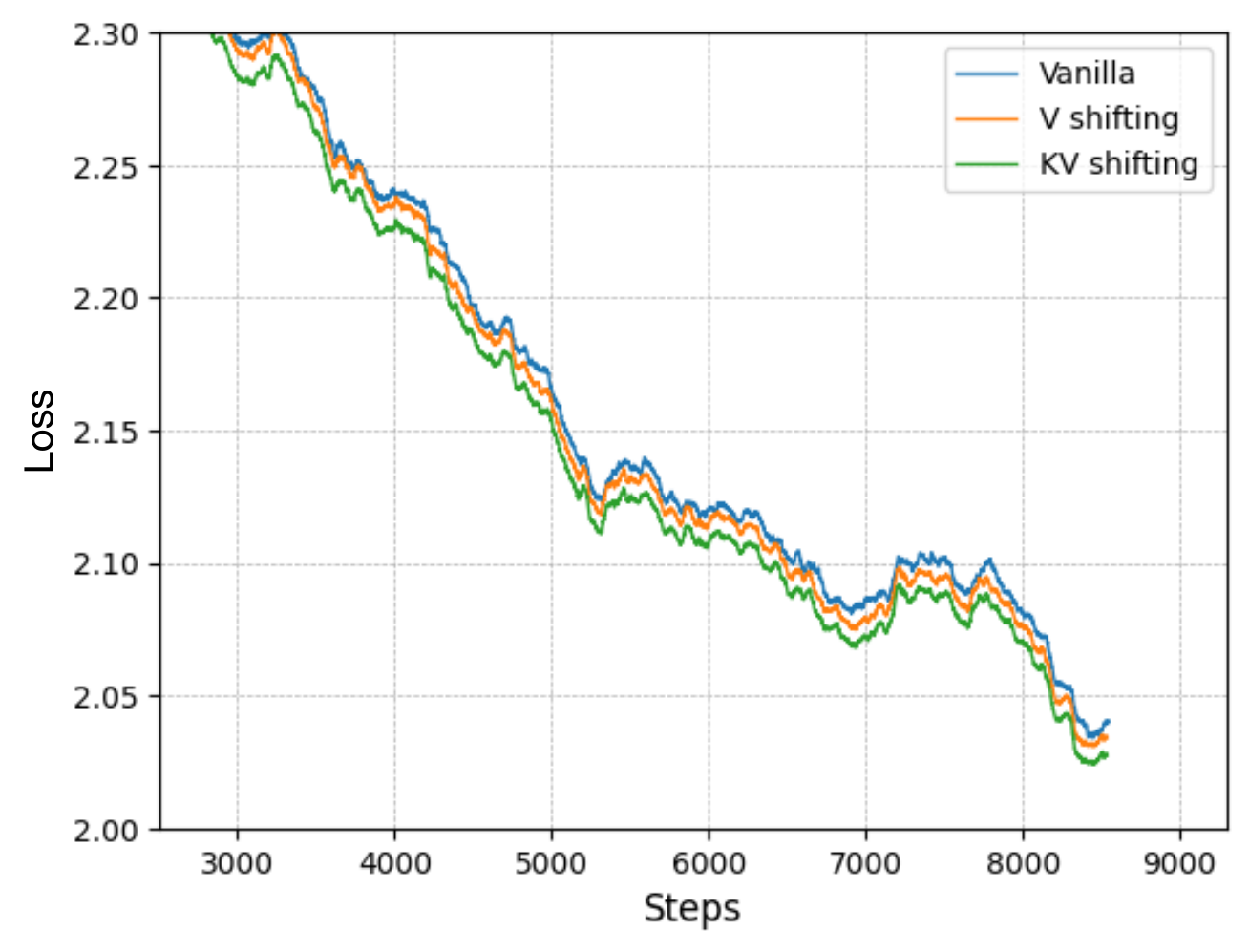
🔼 The figure shows the training loss curves for a 6.7B parameter language model. The graph plots training loss against the number of training steps. Two lines are displayed, one for a model using standard attention and another for a model using KV shifting attention. This visualization allows comparison of the training loss reduction efficiency for both attention mechanisms.
read the caption
(b) 6.7B Parameters

🔼 This figure shows the training loss curve for the 13B parameter model. The loss is plotted against the number of training steps. This plot is part of an experiment comparing the performance of a model using the KV shifting attention mechanism to a vanilla transformer model of the same size. This particular plot shows how the loss function changes over training for the larger model, giving insight into the convergence speed and overall performance of the KV-shifting attention.
read the caption
(c) 13B Parameters

🔼 Figure 6 presents a comparison of training loss curves for transformer language models of varying sizes (1.5B, 6.7B, and 13B parameters). All models were trained on the same amount of data (10 billion tokens). However, the batch size varied across models. The 1.5B and 6.7B parameter models used a batch size of 0.5 million tokens while the 13B parameter model used a batch size of 1 million tokens. This difference in batch size resulted in the 13B model completing approximately half the number of training steps compared to the other two models. The graphs illustrate the training loss over these steps, allowing for a comparison of training efficiency and convergence across model sizes.
read the caption
Figure 6: Training loss comparison between different size. All models are trained on 10B tokens. The batch size for 1.5B and 6.7B model is 0.5M, for 13B is 1M, so the total steps of 13B model is half of others.

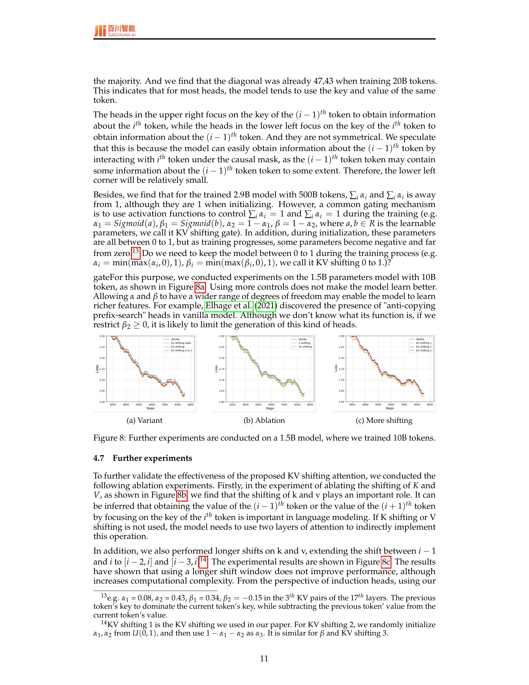
🔼 This figure presents the scaling law for both vanilla attention and KV shifting attention. The x-axis represents the number of parameters (log scale), and the y-axis represents the validation loss (log scale). The plot shows how validation loss decreases as model size increases, illustrating the relationship between model scale and performance for the two different attention mechanisms. This allows comparison of the efficiency with which each attention mechanism utilizes increased model size to improve performance.
read the caption
(a) Scaling law

🔼 The figure shows the training loss curves for a 1.5 billion parameter language model. Specifically, it compares the training loss of a model using standard attention (‘Vanilla’) versus a model using KV shifting attention. The plot shows the loss decreasing over training steps, with KV shifting attention demonstrating faster convergence and a lower final loss compared to the standard model. This illustrates the improved efficiency and effectiveness of the KV shifting attention mechanism for language model training.
read the caption
(b) 1.5B Parameters

🔼 Figure 7 displays the validation loss for models of various sizes trained on 10 billion tokens. The left panel (a) shows a scaling law where the x-axis represents the total number of parameters (excluding embedding parameters) and the y-axis represents the validation loss achieved at the final checkpoint of training. The right panel (b) shows the training loss curve for the 1.5B parameter model, specifically focusing on the model’s performance as the training progressed towards 30B tokens. This highlights how the validation loss remains relatively stable for KV shifting attention, even with a large increase in training data, unlike the vanilla attention model.
read the caption
Figure 7: Validation loss across different size and training tokens. For scaling law, while others in this paper means the total parameters. models are trained on 10B tokens and calculate the final checkpoint’s validation loss.

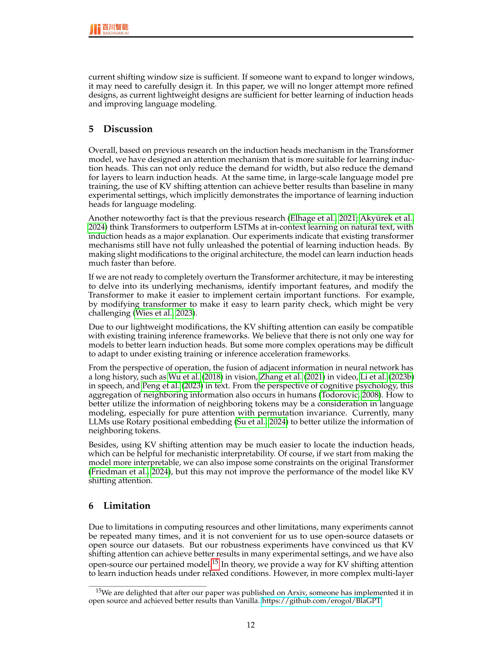
🔼 This figure displays the training loss curves for different variations of the KV shifting attention mechanism on a 1.5B parameter model trained with 10B tokens. The variations include the baseline Vanilla attention, KV shifting attention with a gate mechanism (KV shifting Gate), KV shifting attention restricted to values between 0 and 1 (KV shifting 0 to 1), and standard KV shifting attention. The purpose is to investigate the impact of these modifications on the model’s learning process and performance.
read the caption
(a) Variant

🔼 This ablation study investigates the impact of removing key and value shifting components from the KV shifting attention mechanism. The figure compares the training loss curves of the full KV shifting attention model against versions where either the key shifting or value shifting, or both, are removed. This allows for assessment of the relative contribution of each component to the model’s overall performance and learning ability. Specifically, it shows the impact on the model’s capacity to learn the induction heads mechanism that are central to the paper’s focus on improving language modeling. The relative differences in training loss among these variants illustrate the importance of both key and value shifting for achieving the model’s improved performance.
read the caption
(b) Ablation
More on tables
| Model | Tokens | lambada | winogrande | hellaswag | Arc-E | Arc-C | cmmlu | mmlu | math | average |
|---|---|---|---|---|---|---|---|---|---|---|
| Vanilla - 2.9B | 340B | 52.92 | 52.09 | 42.70 | 27.45 | 25.97 | 28.51 | 29.43 | 0.80 | 32.48 |
| 420B | 52.80 | 54.85 | 43.68 | 28.96 | 26.02 | 34.77 | 30.34 | 1.20 | 34.08 | |
| 500B | 51.66 | 54.06 | 44.49 | 27.90 | 38.22 | 37.26 | 1.80 | 36.45 | ||
| KV Shiting - 2.9B | 340B | 55.44 | 53.91 | 42.87 | 36.74 | 30.04 | 34.51 | 36.20 | 2.00 | 36.46 |
| 420B | 51.91 | 54.78 | 43.83 | 31.91 | 37.24 | 34.30 | 1.80 | 36.55 | ||
| 500B | 54.51 | 44.52 | 39.02 | 30.89 | 40.78 | 40.88 | 2.60 | 38.57 | ||
| Vanilla - 19B | 160B | 59.93 | 48.22 | 48.25 | 30.34 | 24.56 | 39.12 | 39.22 | 1.80 | 36.43 |
| 180B | 58.80 | 48.07 | 47.78 | 31.28 | 25.99 | 40.80 | 39.34 | 2.60 | 36.83 | |
| 200B | 60.88 | 49.01 | 47.36 | 33.25 | 42.92 | 42.68 | 2.60 | 38.06 | ||
| KV shifting - 19B | 160B | 61.93 | 48.46 | 48.28 | 31.25 | 25.06 | 42.10 | 42.87 | 2.00 | 37.74 |
| 180B | 60.20 | 47.67 | 48.16 | 32.45 | 43.38 | 40.49 | 3.00 | 37.74 | ||
| 200B | 62.35 | 48.38 | 48.42 | 33.28 | 29.32 | 42.40 | 43.29 | 3.20 | 38.83 |
🔼 This table presents the results of experiments comparing the performance of language models with and without KV shifting attention. Two model sizes were trained (2.9B and 19B parameters) with different training token counts (500B for 2.9B and 200B for 19B). The table shows the performance of these models on several benchmark datasets (Lambada, Winogrande, HellaSwag, ARC-easy, ARC-Challenge, CMMLU, MMLU, and Math), reporting accuracy scores for each.
read the caption
Table 2: Main results. We trained four models on 2.9B and 19B parameters respectively, with the 2.9B model having a total training token count of 500B and the 19B model having a total training token count of 200B. ARC-E is short for ARC-easy, and ARC-C if short for ARC-Challenge.
| Benchmark | Vanilla | KV shifting | ||||
|---|---|---|---|---|---|---|
| Cloze | Zero | Few | Cloze | Zero | Few | |
| MMLU | 30.41 | 33.14 | 37.26 | 32.17 | 37.13 | 40.88 |
🔼 This table presents a comparison of the performance of the vanilla attention mechanism and the proposed KV shifting attention mechanism on a 2.9B parameter language model trained with 500B tokens. The comparison uses three different evaluation metrics: cloze (zero-shot), zero-shot, and few-shot, showing the model’s performance on various aspects of language understanding. The results highlight the relative performance improvements achieved by using KV shifting attention across multiple evaluation criteria.
read the caption
Table 3: We compare vanilla and KV shifting at 2.9B model with 500B training tokens by using different evaluation metric.
| α₁ > α₂ | α₁ ≤ α₂ | |
|---|---|---|
| β₁ > β₂ | 50 | 17 |
| β₁ ≤ β₂ | 9 | 52 |
🔼 This table presents an analysis of the learnable parameters α₁ and β₁ within the KV shifting attention mechanism of a 2.9B parameter language model trained on 500B tokens. Specifically, it counts how many times the inequalities α₁ ≤ α₂ and β₁ ≤ β₂ hold true across the 128 KV pairs in the model. This analysis helps to understand the learned relationships between these parameters and their impact on the model’s behavior.
read the caption
Table 4: We calculate the number of whether α1≤α2subscript𝛼1subscript𝛼2\alpha_{1}\leq\alpha_{2}italic_α start_POSTSUBSCRIPT 1 end_POSTSUBSCRIPT ≤ italic_α start_POSTSUBSCRIPT 2 end_POSTSUBSCRIPT and β1≤β2subscript𝛽1subscript𝛽2\beta_{1}\leq\beta_{2}italic_β start_POSTSUBSCRIPT 1 end_POSTSUBSCRIPT ≤ italic_β start_POSTSUBSCRIPT 2 end_POSTSUBSCRIPT in each KV pair in 2.9B model with 500B token, the total numbers is 128.
| predict tokens | logit |
|---|---|
| i - 1 | |
| i | |
| i+1 | |
| T | |
| other else | ( |
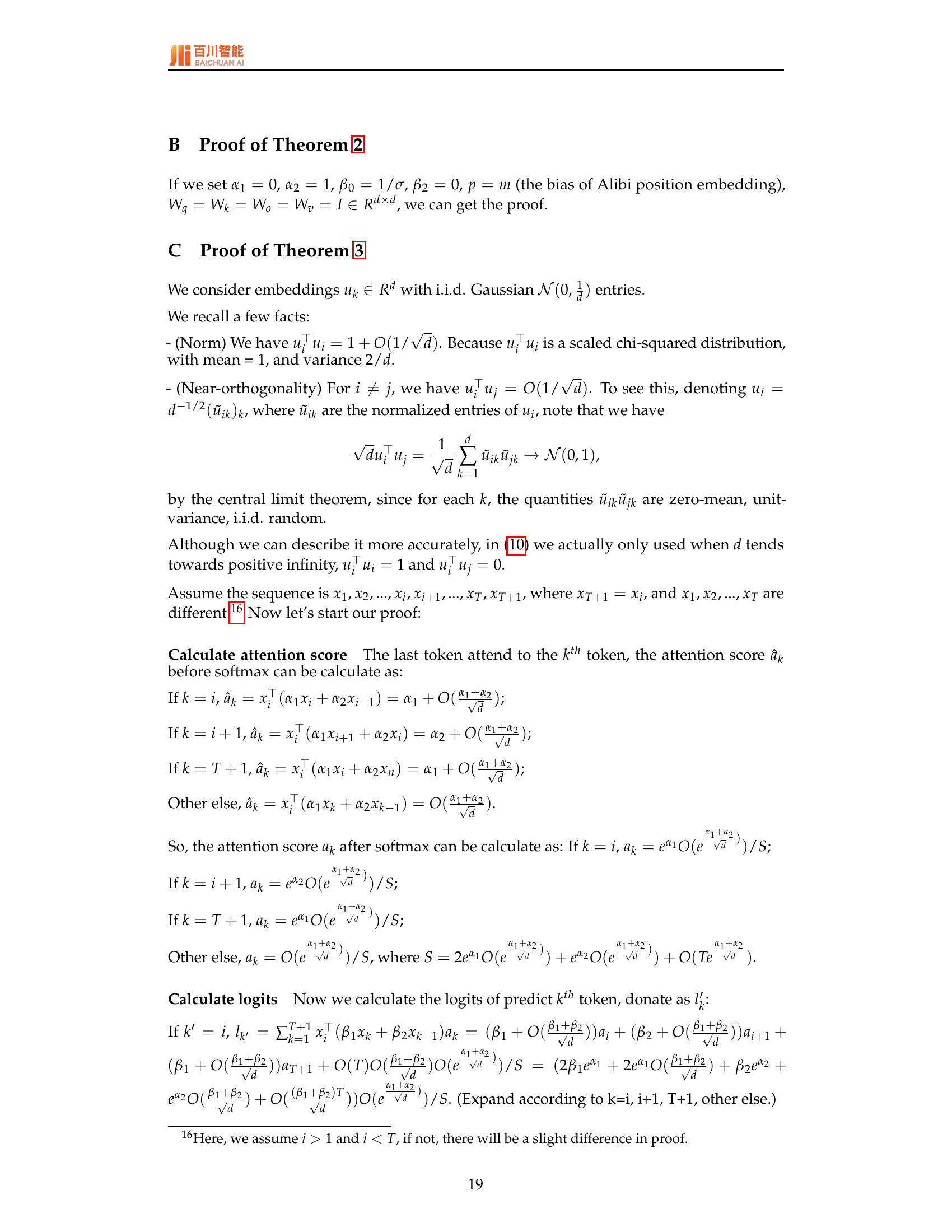
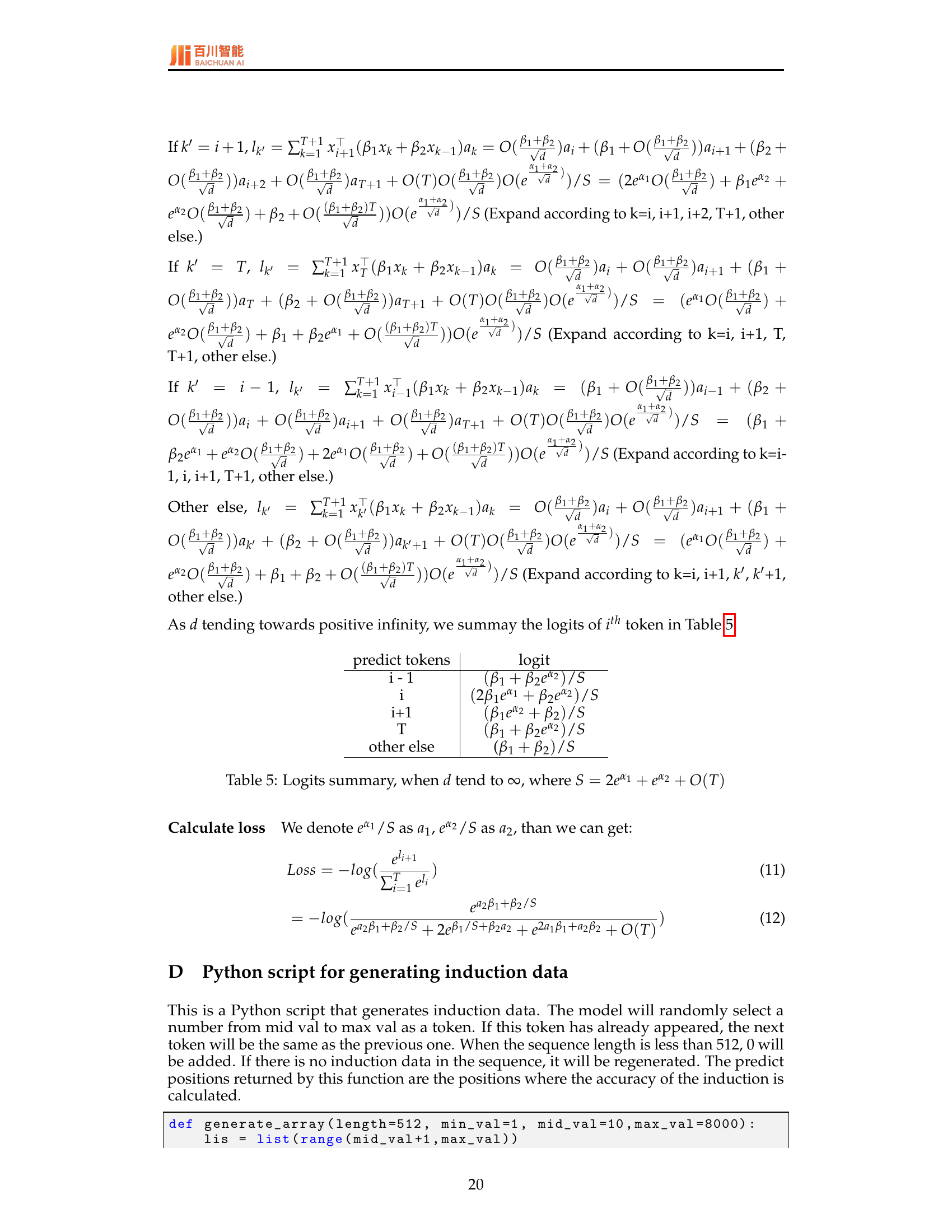
🔼 This table summarizes the logit calculations for predicting different tokens in a simplified model, where the dimensionality (d) approaches infinity. It shows how the logits for predicting the (i-1)th, ith, (i+1)th, and other tokens depend on the learnable parameters α1, α2, β1, β2 and the normalization factor S. The factor S incorporates exponential functions of α1 and α2, indicating how much influence these parameters have on the logits, and also includes a term O(T), which represents an order-of-magnitude factor related to the sequence length (T). This simplified view is used in the theoretical analysis of the learning process, and not necessarily representative of the full model.
read the caption
Table 5: Logits summary, when d𝑑ditalic_d tend to ∞\infty∞, where S=2eα1+eα2+O(T)𝑆2superscript𝑒subscript𝛼1superscript𝑒subscript𝛼2𝑂𝑇S=2e^{\alpha_{1}}+e^{\alpha_{2}}+O(T)italic_S = 2 italic_e start_POSTSUPERSCRIPT italic_α start_POSTSUBSCRIPT 1 end_POSTSUBSCRIPT end_POSTSUPERSCRIPT + italic_e start_POSTSUPERSCRIPT italic_α start_POSTSUBSCRIPT 2 end_POSTSUBSCRIPT end_POSTSUPERSCRIPT + italic_O ( italic_T )
| Parameters | 1.5B | 2.9B | 6.7B | 13B | 19B |
|---|---|---|---|---|---|
| Hidden size | 2,048 | 2,560 | 4,096 | 5,120 | 6,144 |
| Layers | 28 | 32 | 32 | 40 | 48 |
| Head Number | 16 | 20 | 32 | 40 | 48 |
| KV Number | 16 | 4 | 32 | 40 | 4 |
| FFN size | 5,504 | 8,704 | 11,008 | 13,824 | 16,384 |
| Max Length | 2,048 | 4,096 | 2048 | 2,048 | 12,288 |
| Total Tokens | 10B | 500B | 10B | 10B | 200B |
| Vocab size | 36,000 | 48,000 | 36,000 | 36,000 | 48,000 |
| GPU | A100-80G | H800-80G | A100-80G | A100-80G | A800-80G |
| GPU numbers | 64 | 512 | 64 | 128 | 240 |
| Context length | 2,048 | 4,096 | 2,048 | 2,048 | 12,288 |
| Batch size per GPU | 8 | 8 | 8 | 8 | 1 |
| Learning Rate | 2e-4 | 8e-4 | 2e-4 | 2e-4 | 2e-4 |
| Learning Rate shedule | constant | constant | constant | constant | constant |
| Warm-up steps | 1,000 | 600 | 1,000 | 1,000 | 3,000 |
| Optimizer | Adam with α₁=0.9, α₂=0.95, weight decay=0.1 | Adam with α₁=0.9, α₂=0.95, weight decay=0.1 | Adam with α₁=0.9, α₂=0.95, weight decay=0.1 | Adam with α₁=0.9, α₂=0.95, weight decay=0.1 | Adam with α₁=0.9, α₂=0.95, weight decay=0.1 |
| RoPE’s Base | 100,000 | 100,000 | 100,000 | 100,000 | 100,000 |
🔼 This table details the configurations used for training various large language models (LLMs) with different parameter sizes (1.5B, 2.9B, 6.7B, 13B, and 19B). It includes specifications such as hidden size, number of layers, number of heads, feedforward network size, maximum sequence length, vocabulary size, training tokens, GPU type and number, batch size, learning rate, optimizer, and the ROPE (Rotary Position Embedding) base value. The settings reflect choices made for both smaller-scale experiments and for large-scale production-level models.
read the caption
Table 6: Configuration.
| Model | Tr12-Te15 | Tr21-Te24 |
|---|---|---|
| Vanilla | 0.8154 | 0.8711 |
| KV Shifting | 0.8909 | 0.9062 |
🔼 This table presents the results of experiments conducted on the iGSM dataset to evaluate the performance of Vanilla and KV Shifting attention models on grade-school math problems. The experiments are designed to assess the models’ ability to solve math problems with varying complexities. ‘Tr X - Te Y’ indicates that the model was trained on problems with a maximum of X operations and tested on problems with Y operations. The results show the accuracy achieved by each model under these different training and testing conditions, highlighting the impact of the KV Shifting attention mechanism on problem-solving capabilities.
read the caption
Table 7: Experiments on iGSM. Tr X - Te Y means train with the numbers of operation no greater than X and test with the numbers of operation as Y.
Full paper#
