TL;DR#
Current video generation models struggle with producing high-quality, long videos. Existing approaches often result in low resolution or short clips, due to computational costs and limited access to high quality datasets. Furthermore, efficient training methods remain a challenge.
Open-Sora Plan tackles these issues by introducing a novel open-source model. This model incorporates a Wavelet-Flow Variational Autoencoder to reduce memory usage and enhance training speed, and a 3D full attention structure denoiser to improve the quality and length of the videos. The project also proposes various efficient training and inference assistant strategies, including a multi-dimensional data curation pipeline for better data quality.
Key Takeaways#
Why does it matter?#
This paper is crucial for researchers in video generation due to its open-source nature and focus on high-quality, long-duration videos. It offers a novel approach that addresses current limitations in video generation models, opening avenues for further investigation in model architecture, training strategies, and data curation, making significant contributions to the field. Its practical contributions, such as efficient training strategies and data processing pipelines, directly benefit researchers working on similar projects.
Visual Insights#

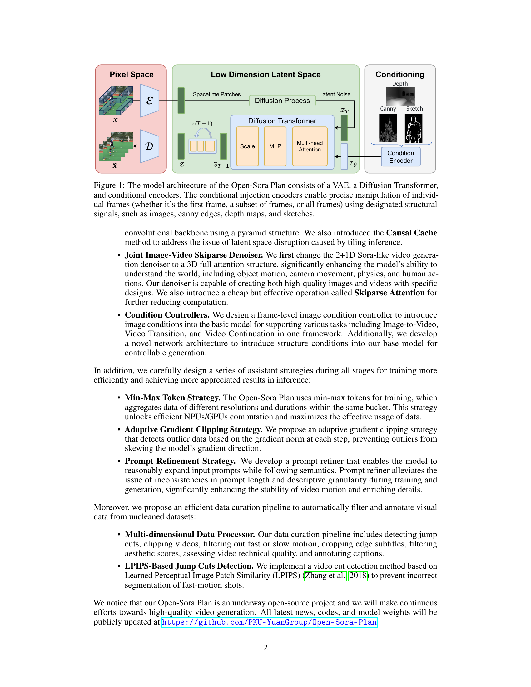
🔼 The figure illustrates the Open-Sora Plan’s video generation model architecture. It’s a three-part system: a Variational Autoencoder (VAE) compresses video frames into a low-dimensional latent space; a Diffusion Transformer processes these latent representations to generate new frames; and conditional encoders allow for fine-grained control over individual frames or sets of frames. These encoders inject various structural signals (images, canny edges, depth maps, and sketches) directly into the generation process, enabling precise manipulation of the generated video’s appearance based on the user’s input.
read the caption
Figure 1: The model architecture of the Open-Sora Plan consists of a VAE, a Diffusion Transformer, and conditional encoders. The conditional injection encoders enable precise manipulation of individual frames (whether it’s the first frame, a subset of frames, or all frames) using designated structural signals, such as images, canny edges, depth maps, and sketches.
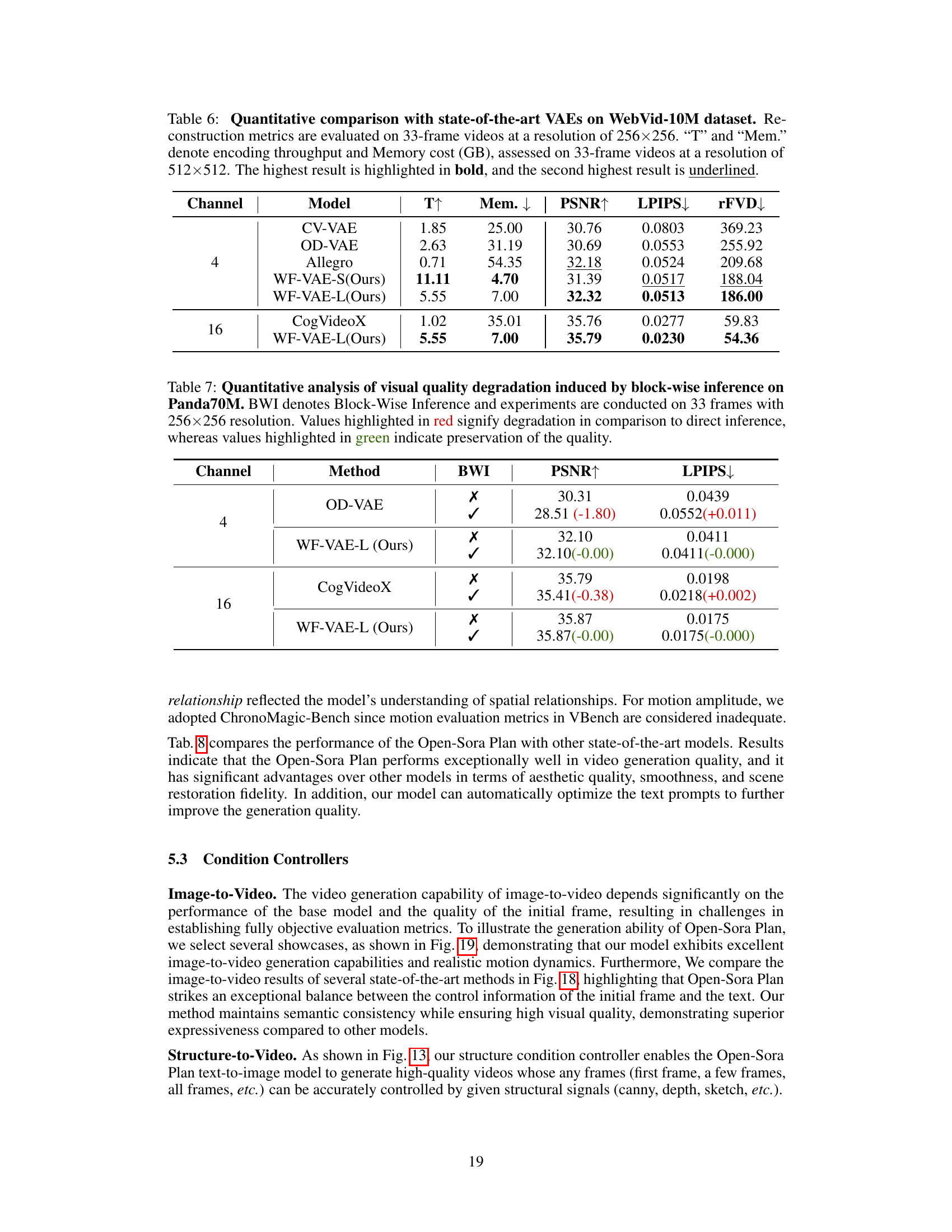
| Attention Mechanisms | Speed | Modeling | Global Attention | Block | Average Attention Distance |
|---|---|---|---|---|---|
| Full 3D Attention | Slow | Strong | All blocks | Equal | 1 |
| 2+1D Attention | Fast | Weak | None block | Not Equal | 2 - (1/T + 1/HW) |
| Skip + Window Attention | Middle | Weak | Half blocks | Not Equal | 2 - (1/k + k/THW) |
| Skiparse Attention | Middle | Strong | All blocks | Equal | 2 - 2/k + 1/k2, 1 < k « THW |
🔼 This table compares different attention mechanisms used in video generation models, specifically focusing on their computational efficiency, modeling capability, and how closely they approximate the performance of the computationally expensive but highly effective Full 3D Attention. The metrics considered include speed, the ability to model spatiotemporal relationships in videos, the proportion of the input data that is involved in attention calculations (Global Attention), and the average distance between tokens considered in attention calculations (Average Attention Distance). The results show that Skiparse Attention offers a good balance between computational efficiency and accuracy, achieving the best spatiotemporal modeling capability among alternatives except for the computationally expensive Full 3D Attention.
read the caption
Table 1: Comparison of the different attention mechanisms. Across multiple comparison metrics, Skiparse Attention is closer to Full 3D Attention, giving it the best spatiotemporal modeling capability apart from Full 3D Attention.
In-depth insights#
Wavelet-Flow VAE#
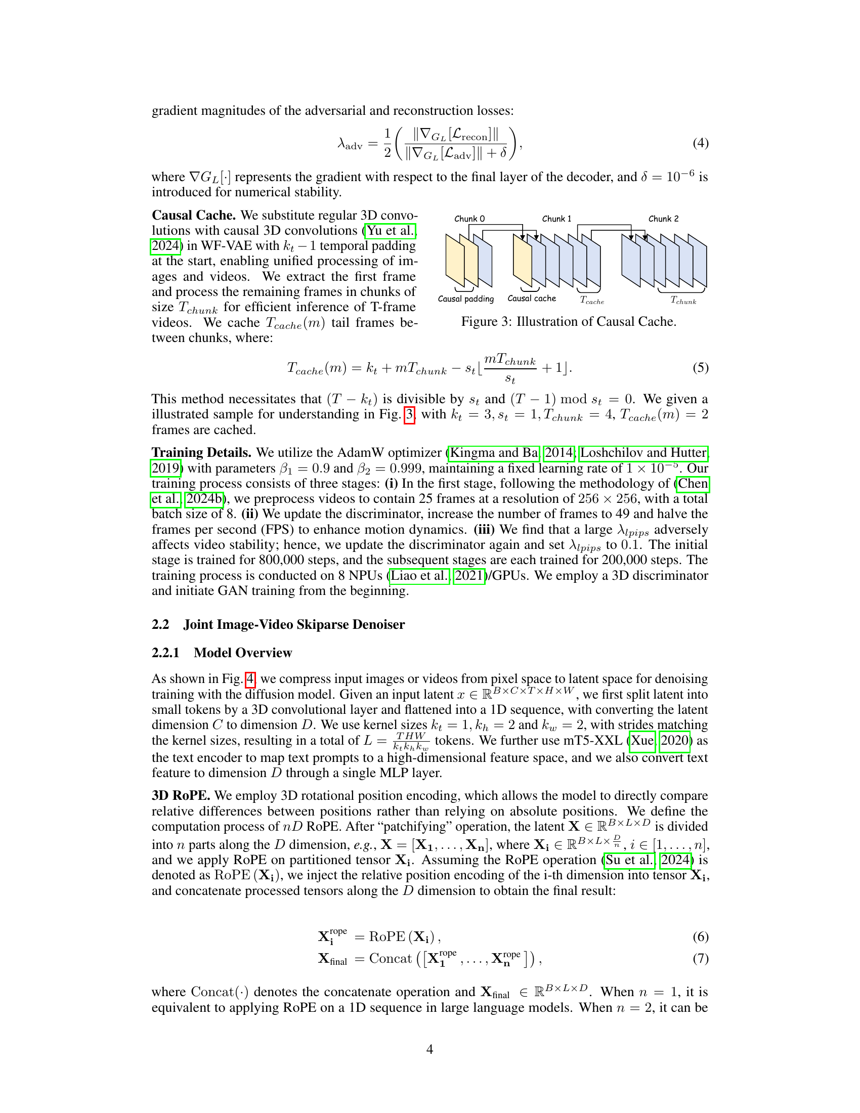
The Wavelet-Flow Variational Autoencoder (WF-VAE) is a crucial component, designed to efficiently learn a compressed representation of video data. Its core innovation lies in leveraging multi-level wavelet transforms to capture multi-scale features in both spatial and temporal dimensions. This approach is particularly beneficial for handling high-resolution videos, as it reduces memory usage and computational cost during training and inference, a common bottleneck in video generation. The WF-VAE’s architecture is designed for symmetry between the encoder and decoder, promoting structural consistency and facilitating better reconstruction. A novel regularization term (LWL) is introduced to further enforce this energy flow, ensuring that important information is preserved during compression and decompression. The training process incorporates several components, including reconstruction loss, adversarial loss, and KL divergence regularization, all carefully balanced to optimize the model’s learning process and the quality of its latent representations. The use of causal caching also enhances inference speed, especially beneficial for long videos.
Skiparse Attention#
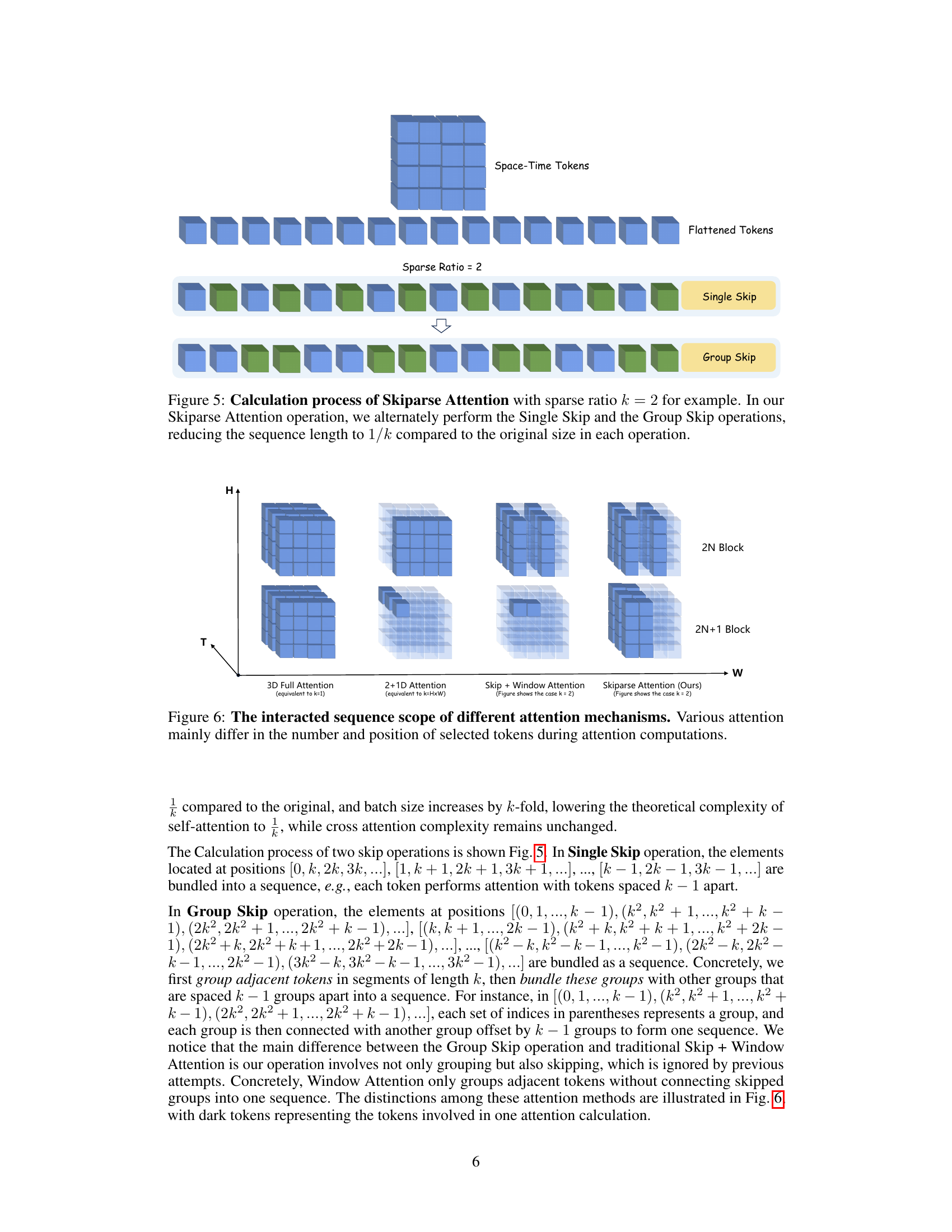
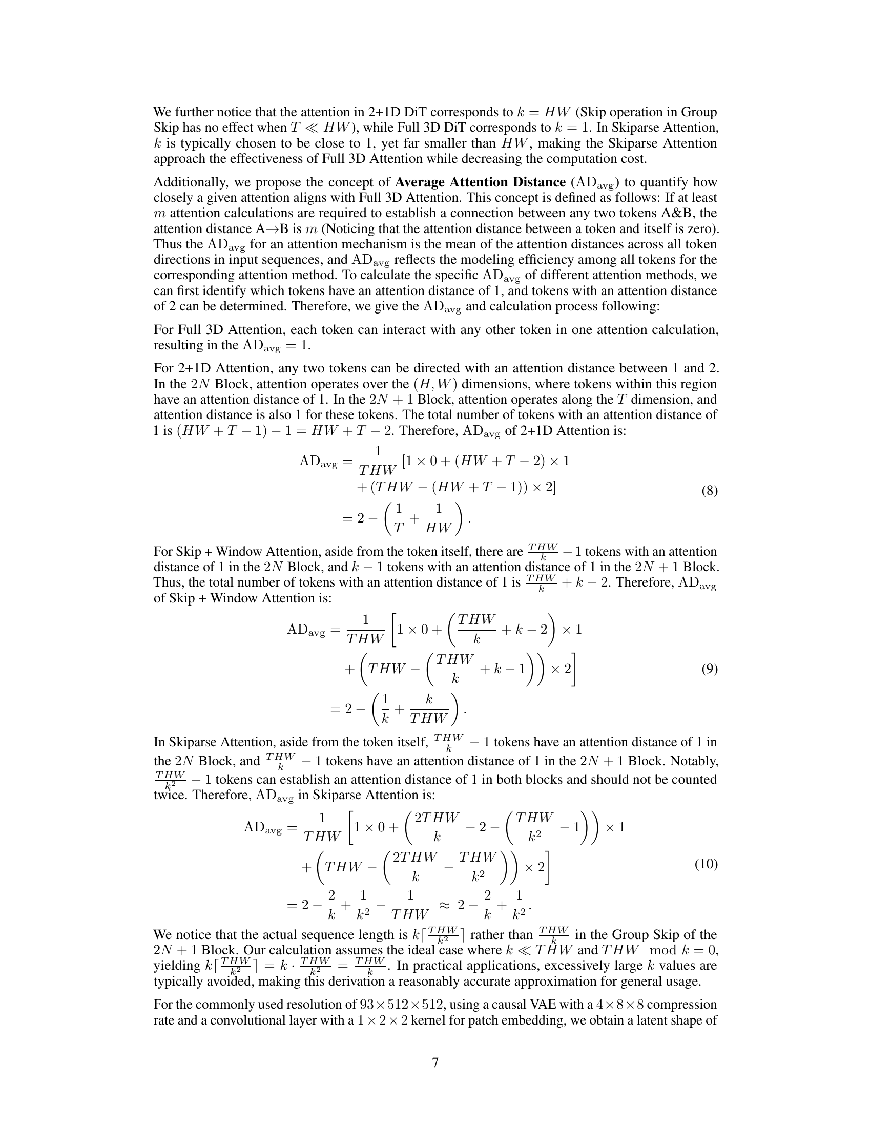
The proposed Skiparse Attention mechanism offers a compelling solution to the computational challenges of full 3D attention in video generation models. By strategically skipping connections between tokens, it significantly reduces the quadratic complexity of self-attention, enhancing training efficiency without severely sacrificing performance. The method cleverly alternates between ‘Single Skip’ and ‘Group Skip’ operations to achieve this, striking a balance between local and global attention. This approach contrasts with simpler methods like 2+1D attention or naive sparse attention, which either severely limit contextual awareness or fall short of achieving the same computational gains. The introduction of the ‘Average Attention Distance’ metric provides a quantifiable measure of how well Skiparse Attention approximates the coverage of full 3D attention, demonstrating its effectiveness in balancing computational cost and model capacity. This thoughtful design makes Skiparse Attention a valuable contribution to the field, paving the way for more computationally efficient and high-quality video generation models.
Conditional Control#
The concept of ‘Conditional Control’ in the context of a large video generation model is crucial for steering the model’s output towards specific user intentions. This involves mechanisms to incorporate diverse conditioning signals, such as text prompts, images, or even structured data like depth maps and sketches, to influence the generated video content. Effective conditional control enables precise manipulation of individual frames or sequences, allowing for fine-grained control over visual elements, motion, and narrative. The success of such a system depends on several key factors: the design of the conditioning encoder, its integration with the video generation architecture, and the training strategies employed. Different approaches to condition injection could involve concatenating features, attention mechanisms, or other methods. Furthermore, it is important to consider the challenges associated with handling diverse conditioning modalities, potentially requiring specialized architectures or training procedures. A well-designed system must balance the flexibility of conditional inputs with the need for stable and coherent video outputs, avoiding artifacts or inconsistencies. Ultimately, the goal is to empower users with the ability to easily and intuitively control the generation process, creating a powerful and versatile tool for video creation.
Training Strategies#
The research paper details various training strategies employed to enhance the efficiency and effectiveness of the video generation model. A key strategy is the ‘Min-Max Token’ approach, which tackles the challenge of variable-length video data by using min-max tokens to create uniform batch sizes, optimizing computational resources. Adaptive Gradient Clipping addresses the issue of loss spikes during training, a problem common in large-scale models, by dynamically adjusting gradient thresholds based on moving averages. This approach maintains training stability without sacrificing model quality. Further enhancing the model, a prompt refiner strategically improves input prompts, bridging the gap between concise user input and lengthy training data, leading to more consistent and detailed video outputs. These strategies, coupled with multi-stage training and carefully selected datasets, significantly contribute to the model’s ability to generate high-quality, long-duration videos.
Future Directions#
The paper’s exploration of future directions in video generation highlights several key areas. Scaling up model size is crucial, as larger models have shown increased understanding of physical laws and improved generation quality. This requires efficient training strategies like improved parallelization techniques to manage the computational demands. The research also emphasizes the need for more diverse and complex datasets. The current datasets lack sufficient variety in scenes, actions, and camera movements, limiting the model’s ability to handle diverse scenarios and generate truly realistic videos. Addressing this involves curating datasets with richer annotations including camera movement, video style, motion speed, and potentially cross-modal information like audio. Improved evaluation metrics are also vital, moving beyond current limitations and incorporating human evaluation where appropriate. Finally, efficient algorithms and architectures should be developed to facilitate training and inference on larger models and more complex data. Exploring architectures beyond the current design to maximize efficiency is also highlighted. The overall direction emphasizes a balanced approach combining model scaling, data enhancement, and evaluation advancements for achieving next-generation video generation models.
More visual insights#
More on figures

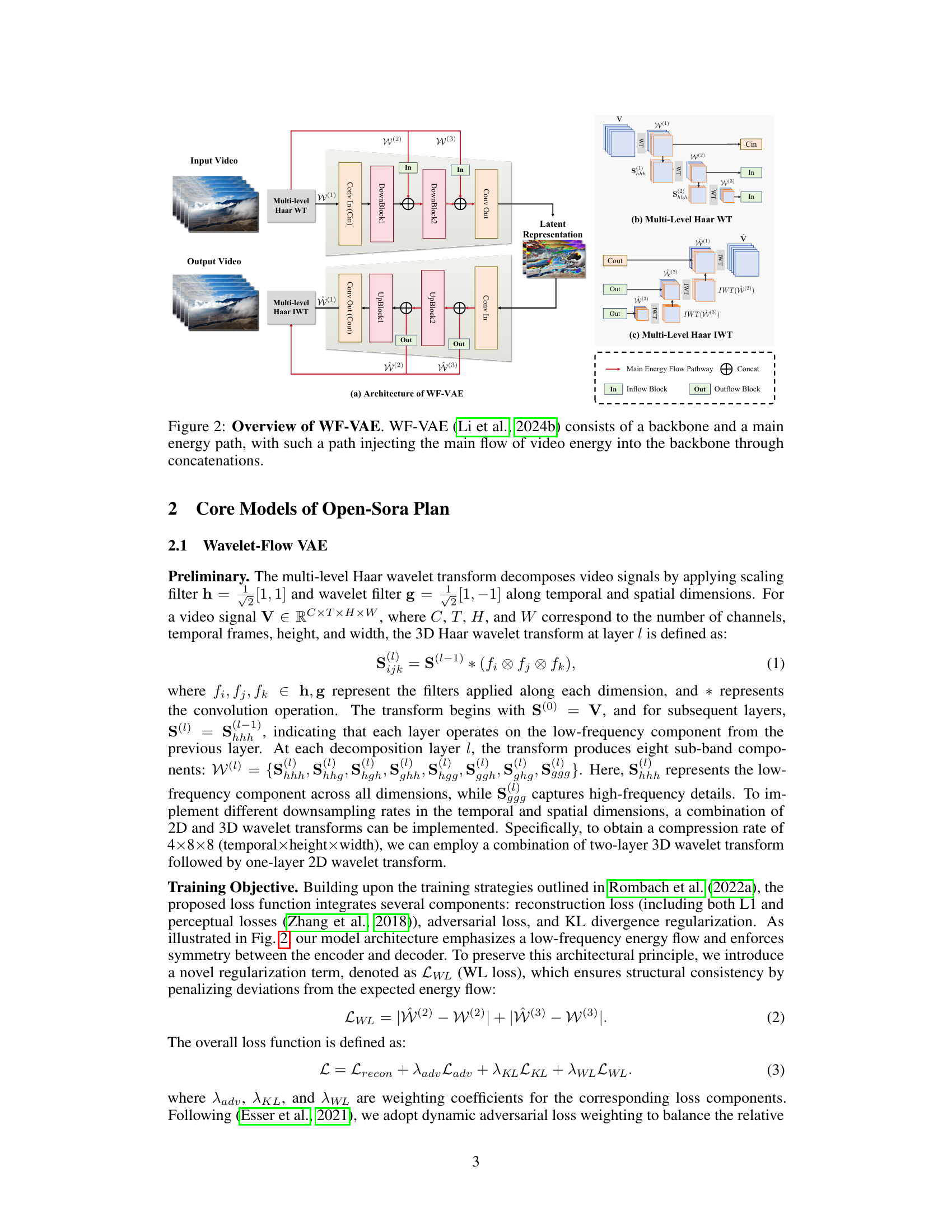
🔼 Figure 2 illustrates the architecture of the Wavelet-Flow Variational Autoencoder (WF-VAE). The WF-VAE processes video data by using a multi-level Haar wavelet transform to decompose the video into different frequency components (low-frequency and high-frequency details). This decomposition allows for efficient processing and compression of the video data. A main energy path carries the core video information through the network, while the backbone integrates the processed wavelet components. The main energy path’s information is combined with the backbone’s output through concatenation, ensuring that important video features are preserved throughout the process. This design enhances training speed and reduces memory usage, making it efficient for handling high-resolution videos.
read the caption
Figure 2: Overview of WF-VAE. WF-VAE [li2024wfvaeenhancingvideovae] consists of a backbone and a main energy path, with such a path injecting the main flow of video energy into the backbone through concatenations.

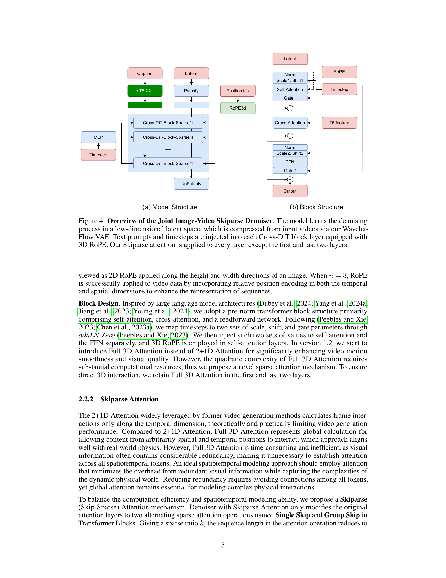
🔼 The figure illustrates the architecture of the Joint Image-Video Skiparse Denoiser, a key component of the Open-Sora Plan video generation model. The model operates in a low-dimensional latent space, derived from input videos compressed using the Wavelet-Flow VAE (Variational Autoencoder). This latent space representation is processed through a series of Cross-DiT (Cross-Dimensional Transformer) blocks. Each block incorporates both text prompts and timestep information (indicating the stage of the denoising process), enhanced by a 3D Rotational Positional Encoding (ROPE) mechanism to handle spatio-temporal dependencies effectively. Notably, a Skiparse attention mechanism is implemented in all but the first and last two Cross-DiT blocks. This Skiparse attention is a computationally efficient variant of full 3D attention that enhances performance and reduces memory usage, making it suitable for large-scale video generation.
read the caption
Figure 3: Overview of the Joint Image-Video Skiparse Denoiser. The model learns the denoising process in a low-dimensional latent space, which is compressed from input videos via our Wavelet-Flow VAE. Text prompts and timesteps are injected into each Cross-DiT block layer equipped with 3D RoPE. Our Skiparse attention is applied to every layer except the first and last two layers.

🔼 Figure 4 illustrates the Skiparse Attention mechanism, a computationally efficient attention method used in the Open-Sora Plan’s video generation model. The figure uses a sparse ratio (k) of 2 to demonstrate how it reduces computational cost. The core idea is to alternate between ‘Single Skip’ and ‘Group Skip’ operations. In a Single Skip operation, only every k-th token (in this case, every second token) participates in the attention calculation, reducing the number of attention computations. The Group Skip operation groups tokens into blocks of size k and then selectively samples from these blocks to participate in the attention mechanism. By alternating these two skip operations, the effective sequence length is reduced to 1/k of the original, thus significantly decreasing the computational complexity.
read the caption
Figure 4: Calculation process of Skiparse Attention with sparse ratio k=2𝑘2k=2italic_k = 2 for example. In our Skiparse Attention operation, we alternately perform the Single Skip and the Group Skip operations, reducing the sequence length to 1/k1𝑘1/k1 / italic_k compared to the original size in each operation.
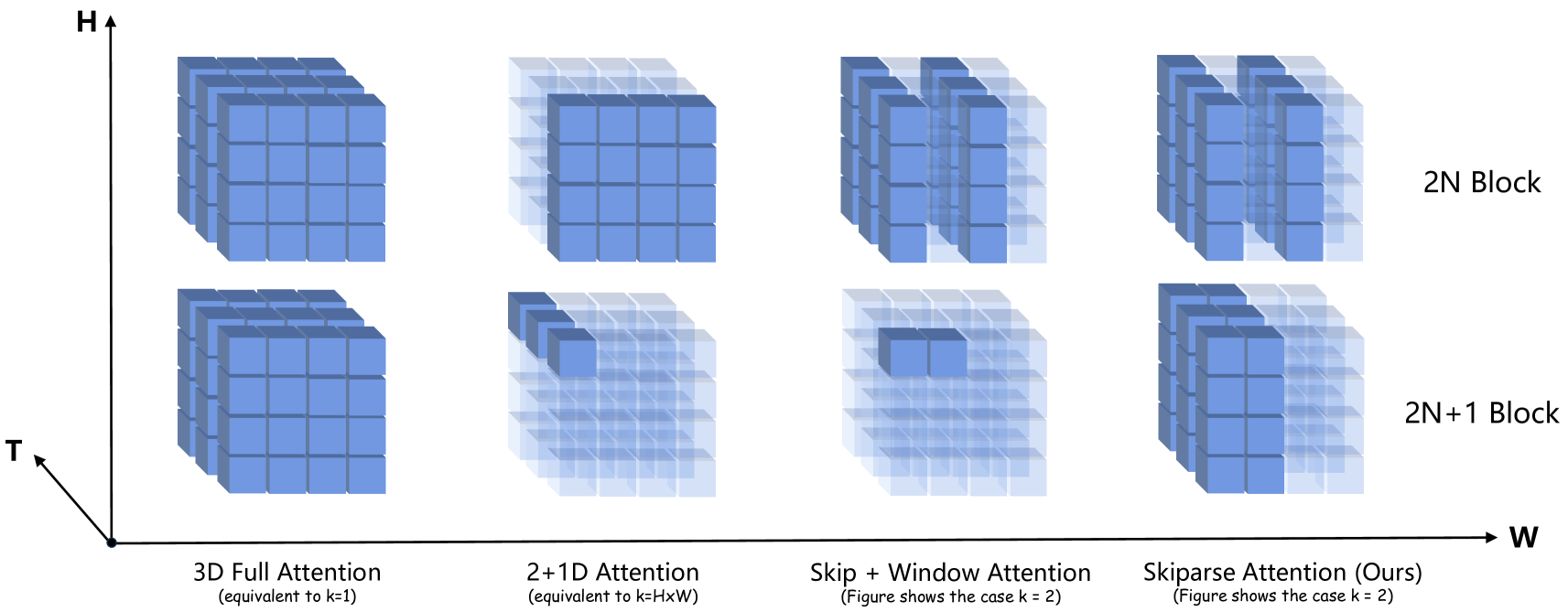
🔼 Figure 5 illustrates the differences in how various attention mechanisms select tokens for processing within a sequence. It visually compares four different attention methods: Full 3D Attention, 2+1D Attention, Skip + Window Attention, and Skiparse Attention (the proposed method). Each method is shown alongside a visual representation of the sequence of tokens and which tokens are considered during the attention calculations. The main difference between these methods lies in the number of tokens selected and their positions within the sequence, directly influencing computational cost and the scope of information considered for each attention operation. The figure highlights that the Skiparse Attention method strikes a balance between computational efficiency and the ability to capture long-range dependencies, which is a key aspect of the paper’s contribution.
read the caption
Figure 5: The interacted sequence scope of different attention mechanisms. Various attention mainly differ in the number and position of selected tokens during attention computations.

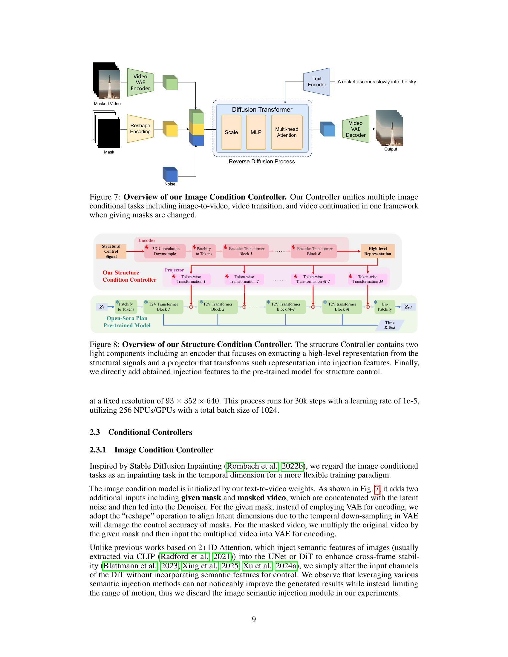
🔼 The figure illustrates the architecture of an Image Condition Controller designed for versatile video generation tasks. It integrates multiple conditional inputs, including image-to-video generation, video transition, and video continuation. The controller leverages a masked video input, allowing for precise manipulation of individual frames. The architecture comprises a VAE encoder to extract image features, which are then combined with latent noise and text embeddings in a Diffusion Transformer. The output is then passed through a VAE decoder to generate the desired video frames. The use of masks enables the unified handling of various image conditioning tasks within a single framework.
read the caption
Figure 6: Overview of our Image Condition Controller. Our Controller unifies multiple image conditional tasks including image-to-video, video transition, and video continuation in one framework when giving masks are changed.

🔼 The Structure Condition Controller efficiently adds structural control to the base model by using two lightweight components: an encoder and a projector. The encoder processes the structural signals (like canny edges, depth maps, or sketches) to extract a high-level representation. This representation is then transformed by the projector into injection features. These features are directly added to the pre-trained model’s corresponding transformer block to enable structure control during video generation.
read the caption
Figure 7: Overview of our Structure Condition Controller. The structure Controller contains two light components including an encoder that focuses on extracting a high-level representation from the structural signals and a projector that transforms such representation into injection features. Finally, we directly add obtained injection features to the pre-trained model for structure control.

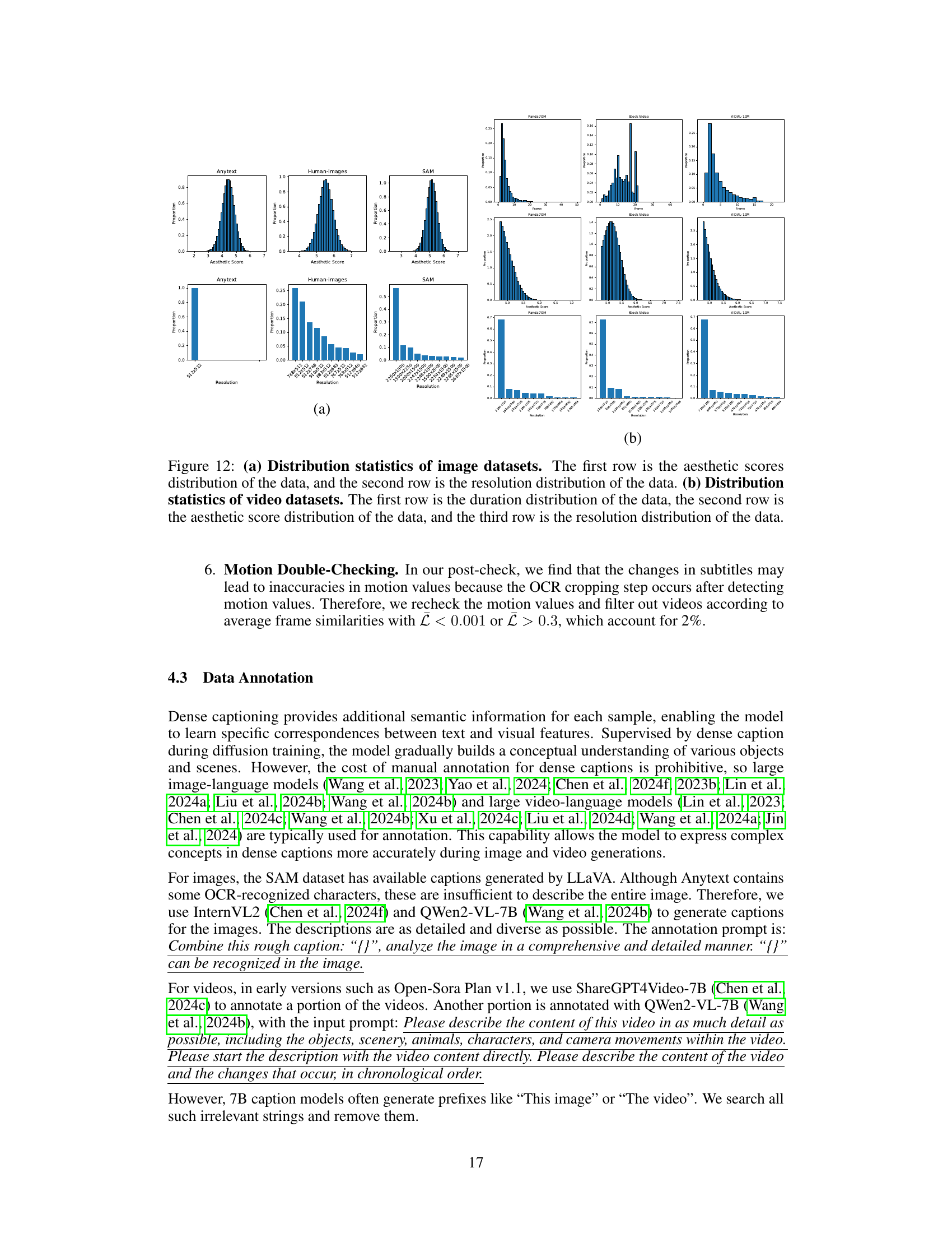
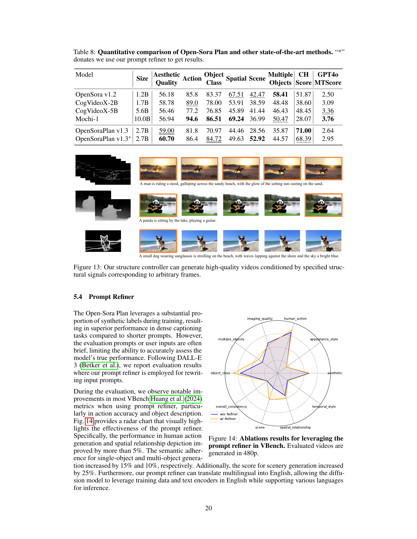
🔼 The figure shows the distribution statistics of image datasets. The first row presents histograms illustrating the distribution of aesthetic scores for three different datasets: Anytext, Human-images, and SAM. The second row displays histograms showing the distribution of resolutions (image dimensions) for the same three datasets. The distributions reveal variations in aesthetic quality and resolution among the datasets.
read the caption
(a)

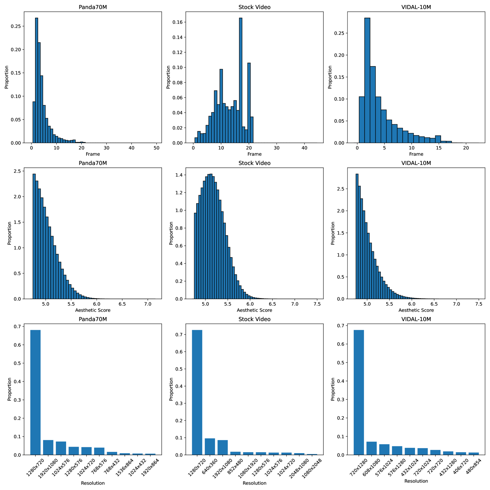
🔼 Figure 12(b) shows the distribution statistics of video datasets used in the Open-Sora Plan project. It presents three rows of histograms, each row representing a different aspect of the video data. The first row visualizes the distribution of video durations across various lengths. The second row displays the distribution of aesthetic scores assigned to the videos, reflecting their perceived visual quality. The third row shows the distribution of video resolutions, indicating the variety of video dimensions included in the dataset. This figure helps to characterize the dataset used for training and evaluating the Open-Sora video generation model.
read the caption
(b)
🔼 The figure shows a comparison among several state-of-the-art methods in Image-to-Video tasks. Two example image-to-video generations are presented, each with the same prompt given to different models. This allows for a visual comparison of the quality and style of video generated by each model. Specifically, it highlights the differences in the realism, detail, and overall fidelity of the generated videos.
read the caption
(c)

🔼 The figure shows the distribution statistics of video datasets. Specifically, the first row displays the distribution of video durations, the second row shows the distribution of aesthetic scores, and the third row shows the distribution of resolutions. Each row contains histograms for three different datasets: Panda70M, Stock Video, and VIDAL-10M.
read the caption
(d)

🔼 This figure shows a comparison of different video generation methods on the task of generating videos from text descriptions. The figure shows several state-of-the-art methods, along with OpenSora, on two different video generation examples. Each example has multiple generated videos from multiple methods to visually compare their relative performance.
read the caption
(e)

🔼 This figure shows the qualitative comparison of several state-of-the-art video generation methods on a dynamic scene with motion blur. The ground truth video is compared to the results generated by WF-VAE-L(Chn=16), CogVideo-X(Chn=16), WF-VAE-L, WF-VAE-S, Allegro, and OD-VAE. The comparison highlights the differences in reconstruction quality and visual fidelity across different methods, demonstrating the superior performance of WF-VAE in handling dynamic scenes with motion blur.
read the caption
(f)

🔼 This figure shows a qualitative comparison of several state-of-the-art video generation models on the task of generating videos from text prompts. The specific text prompt used is ‘A cinematic wide portrait of a man with his face lit by the glow of a TV.’ The figure presents the generated videos by different models in a grid format, allowing for a direct visual comparison. The quality and style of the generated videos are assessed based on various factors such as realism, details, motion smoothness, and overall visual appeal.
read the caption
(g)
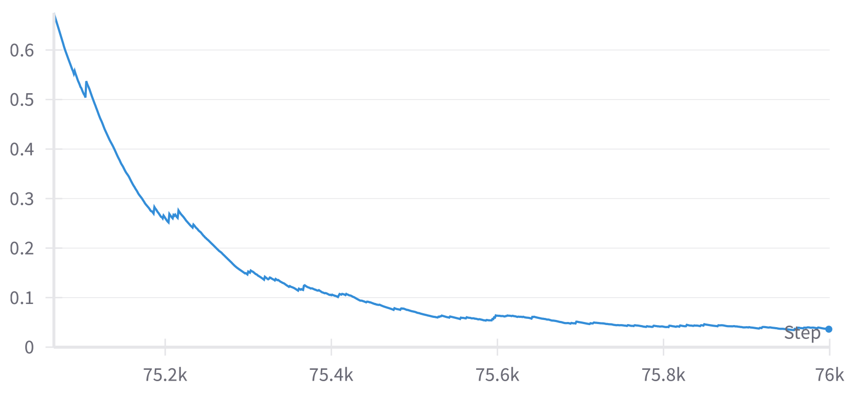
🔼 EMA of the variance of the maximum gradient norm. This plot shows the exponential moving average (EMA) of the variance of the maximum gradient norm across all NPUs/GPUs. The EMA smooths out fluctuations in the variance, making it easier to see overall trends and identify potential issues. A sudden increase in this value might indicate the presence of outliers in the training data or problems with the training process.
read the caption
(h)

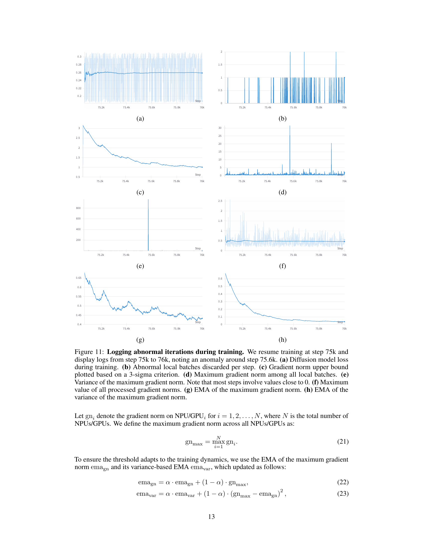
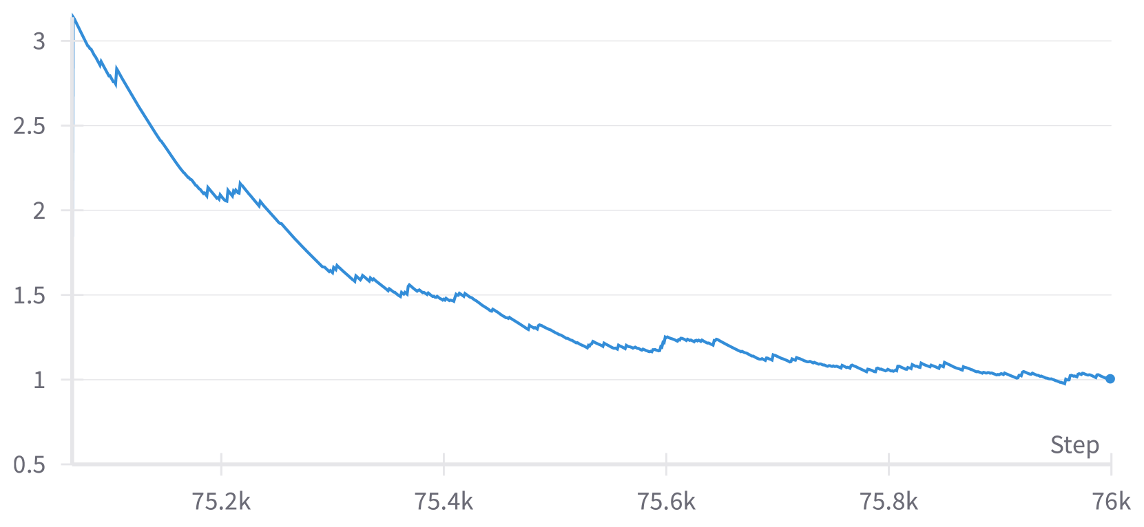
🔼 Figure 8 illustrates the effects of an anomaly detected during training of a diffusion model. The training was resumed at step 75,000, and data from steps 75,000 to 76,000 are displayed. A key anomaly is observed around step 75,600. The figure shows eight plots: (a) The overall diffusion model loss during training. (b) Number of abnormal local batches discarded at each step. (c) Upper bound for the gradient norm, calculated using a 3-sigma criterion. (d) Maximum gradient norm across all local batches in each step. (e) Variance of the maximum gradient norm. (f) The maximum value of all processed gradient norms. (g) Exponential Moving Average (EMA) of the maximum gradient norm. (h) EMA of the variance of the maximum gradient norm. This detailed breakdown helps to visually understand how the proposed adaptive gradient clipping strategy responds to and mitigates anomalies during model training, preserving stability and output quality.
read the caption
Figure 8: Logging abnormal iterations during training. We resume training at step 75k and display logs from step 75k to 76k, noting an anomaly around step 75.6k. (a) Diffusion model loss during training. (b) Abnormal local batches discarded per step. (c) Gradient norm upper bound plotted based on a 3-sigma criterion. (d) Maximum gradient norm among all local batches. (e) Variance of the maximum gradient norm. Note that most steps involve values close to 0. (f) Maximum value of all processed gradient norms. (g) EMA of the maximum gradient norm. (h) EMA of the variance of the maximum gradient norm.
🔼 The figure shows the distribution statistics of image datasets. The first row displays the distribution of aesthetic scores, while the second row shows the distribution of resolutions. Specifically, it presents the top 10 most frequent resolutions for the Anytext, Human-images, and SAM datasets, alongside histograms illustrating the distribution of aesthetic scores for each dataset. The distributions reveal differences in terms of resolution variety and aesthetic score ranges across these datasets. For example, the Anytext dataset shows a unified resolution (512x512), while Human-images and SAM demonstrate greater diversity in resolution and aesthetic scores.
read the caption
(a)

🔼 This figure shows the distribution statistics of video datasets. The first row presents the distribution of video durations. The second row displays the distribution of aesthetic scores. The third row illustrates the distribution of resolutions.
read the caption
(b)
More on tables
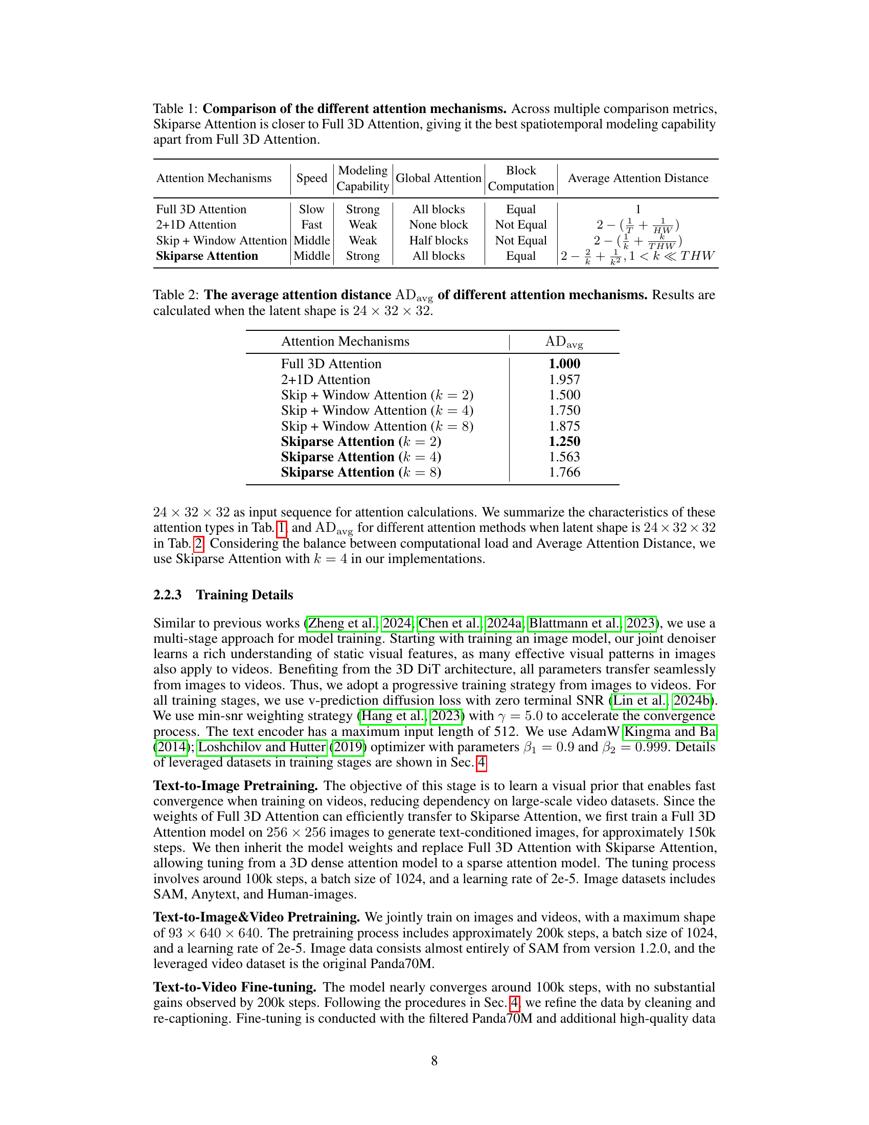
| Attention Mechanisms | ADavg |
|---|---|
| Full 3D Attention | 1.000 |
| 2+1D Attention | 1.957 |
| Skip + Window Attention (k=2) | 1.500 |
| Skip + Window Attention (k=4) | 1.750 |
| Skip + Window Attention (k=8) | 1.875 |
| Skiparse Attention (k=2) | 1.250 |
| Skiparse Attention (k=4) | 1.563 |
| Skiparse Attention (k=8) | 1.766 |
🔼 This table presents a comparison of different attention mechanisms used in video generation models, specifically focusing on the concept of ‘Average Attention Distance (ADavg)’. ADavg quantifies how closely the attention patterns of a given mechanism resemble those of a full 3D attention mechanism, which is computationally expensive but provides the most comprehensive context. Lower ADavg values generally indicate a more efficient mechanism that still captures significant spatiotemporal relationships, though with less computational cost. The results shown are calculated for a specific latent space size of 24x32x32, which is a parameter within the video generation model and impacts the attention calculations. Different attention mechanisms (Full 3D Attention, 2+1D Attention, Skip+Window Attention, and Skiparse Attention) are compared based on their ADavg, illustrating the trade-offs between computational cost and the comprehensiveness of attention.
read the caption
Table 2: The average attention distance ADavgsubscriptADavg\mathrm{AD_{avg}}roman_AD start_POSTSUBSCRIPT roman_avg end_POSTSUBSCRIPT of different attention mechanisms. Results are calculated when the latent shape is 24×32×3224323224\times 32\times 3224 × 32 × 32.
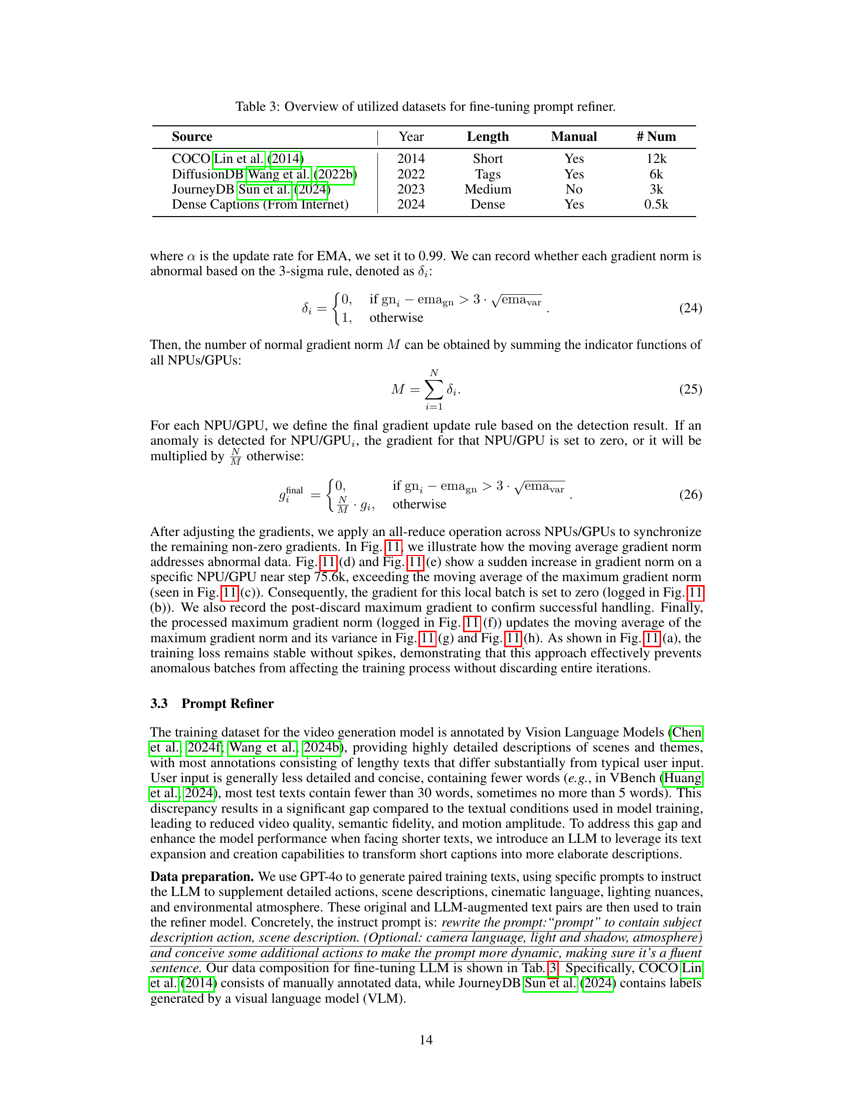
| Source | Year | Length | Manual | # Num |
|---|---|---|---|---|
| COCO [lin2014microsoft] | 2014 | Short | Yes | 12k |
| DiffusionDB [wang2022diffusiondb] | 2022 | Tags | Yes | 6k |
| JourneyDB [sun2024journeydb] | 2023 | Medium | No | 3k |
| Dense Captions (From Internet) | 2024 | Dense | Yes | 0.5k |
🔼 This table details the datasets used to fine-tune the prompt refiner model. It lists the source of each dataset, the year it was published, the length of captions typically found within, whether the captions were manually created or automatically generated, and the total number of data points in each.
read the caption
Table 3: Overview of utilized datasets for fine-tuning prompt refiner.
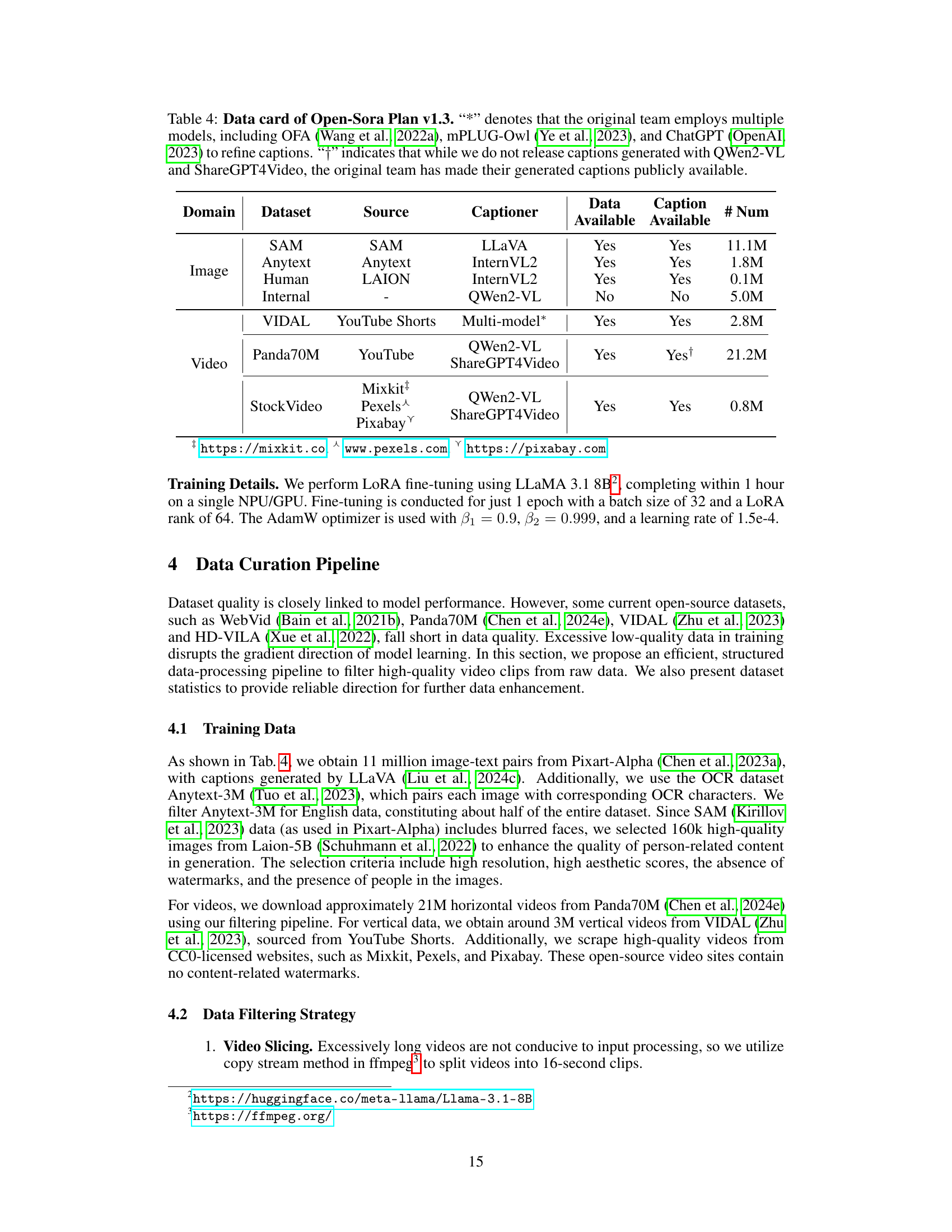
| Domain | Dataset | Source | Captioner | Data Available | Caption Available | # Num |
|---|---|---|---|---|---|---|
| Image | SAM | SAM | LLaVA | Yes | Yes | 11.1M |
| Anytext | Anytext | InternVL2 | Yes | Yes | 1.8M | |
| Human | LAION | InternVL2 | Yes | Yes | 0.1M | |
| Internal | - | QWen2-VL | No | No | 5.0M | |
| Video | VIDAL | YouTube Shorts | Multi-model∗ | Yes | Yes | 2.8M |
| Panda70M | YouTube | QWen2-VL | Yes | Yes† | 21.2M | |
| ShareGPT4Video | ||||||
| StockVideo | Mixkit‡ | QWen2-VL | Yes | Yes | ||
| Pexels⋏ | ShareGPT4Video | 0.8M | ||||
| Pixabay⋎ |
🔼 This table presents a detailed data card for Open-Sora Plan version 1.3, outlining the datasets used for training the model. It specifies the domain (image or video), the dataset name, the source of the data, the caption generator used, and the availability of both the data and captions. Noteworthy is that the original creators employed multiple models (OFA, mPLUG-Owl, and ChatGPT) for caption refinement, and while the current work doesn’t share captions generated using QWen2-VL and ShareGPT4Video, the original team’s generated captions are publicly available. The table provides a comprehensive overview of the data resources leveraged in the Open-Sora Plan model, detailing their origins and accessibility.
read the caption
Table 4: Data card of Open-Sora Plan v1.3. “*” denotes that the original team employs multiple models, including OFA [wang2022ofa], mPLUG-Owl [ye2023mplug], and ChatGPT [openai2023gpt4] to refine captions. “††{\dagger}†” indicates that while we do not release captions generated with QWen2-VL and ShareGPT4Video, the original team has made their generated captions publicly available.
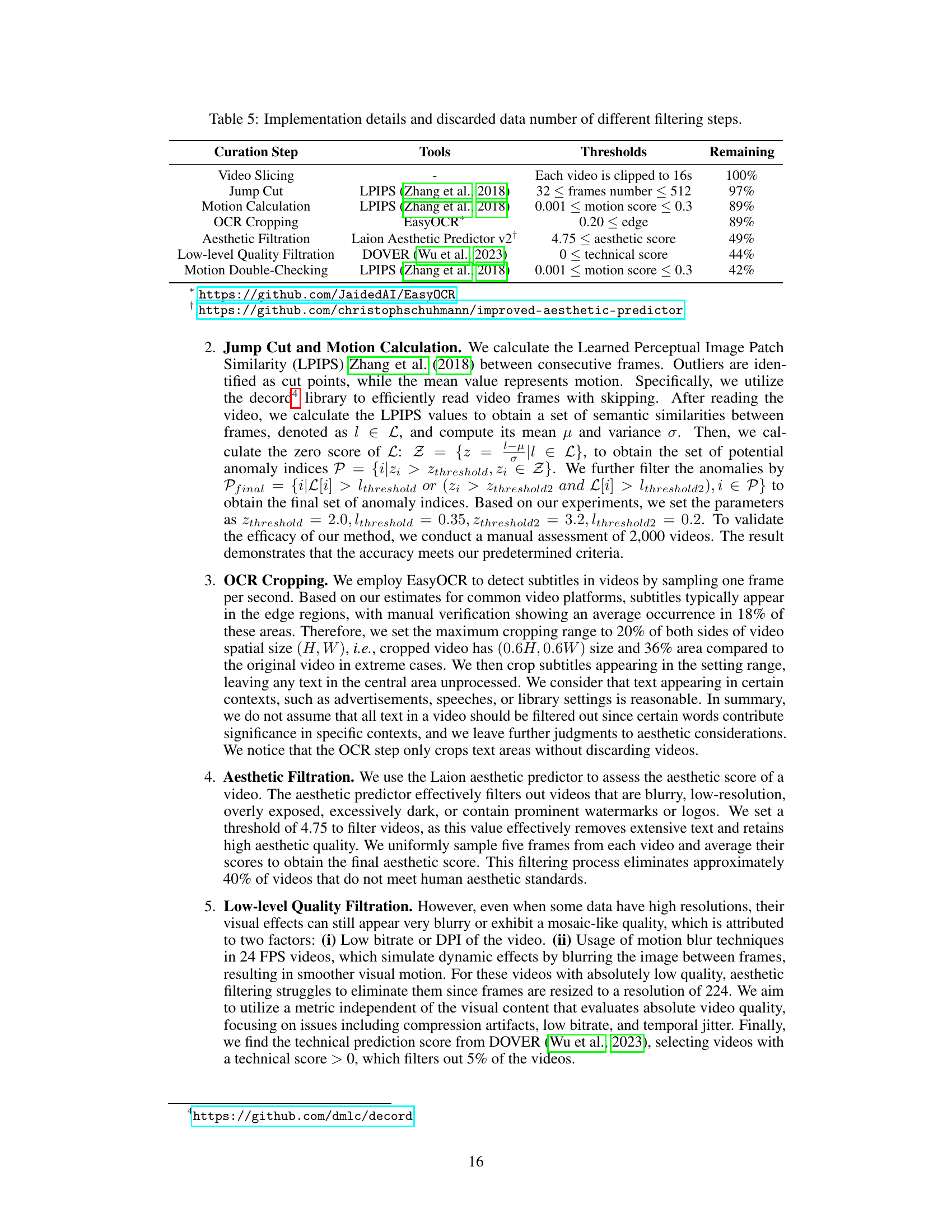
| Curation Step | Tools | Thresholds | Remaining |
|---|---|---|---|
| Video Slicing | - | Each video is clipped to 16s | 100% |
| Jump Cut | LPIPS [Zhang_Isola_Efros_Shechtman_Wang_2018] | 32 ≤ frames number ≤ 512 | 97% |
| Motion Calculation | LPIPS [Zhang_Isola_Efros_Shechtman_Wang_2018] | 0.001 ≤ motion score ≤ 0.3 | 89% |
| OCR Cropping | EasyOCR* | 0.20 ≤ edge | 89% |
| Aesthetic Filtration | Laion Aesthetic Predictor v2† | 4.75 ≤ aesthetic score | 49% |
| Low-level Quality Filtration | DOVER [wu2023exploring] | 0 ≤ technical score | 44% |
| Motion Double-Checking | LPIPS [Zhang_Isola_Efros_Shechtman_Wang_2018] | 0.001 ≤ motion score ≤ 0.3 | 42% |
🔼 This table details the data filtering process used in the Open-Sora Plan project. Each row represents a step in the curation pipeline, specifying the techniques used (like jump cut detection with LPIPS or aesthetic score filtering), the thresholds applied to determine whether to discard data, and the resulting dataset size after each filtering step. It shows how the raw dataset is refined through multiple stages to improve data quality for training the video generation model. This process is crucial to the models performance.
read the caption
Table 5: Implementation details and discarded data number of different filtering steps.
| Channel | Model | T↑ | Mem.↓ | PSNR↑ | LPIPS↓ | rFVD↓ |
|---|---|---|---|---|---|---|
| 4 | CV-VAE | 1.85 | 25.00 | 30.76 | 0.0803 | 369.23 |
| 4 | OD-VAE | 2.63 | 31.19 | 30.69 | 0.0553 | 255.92 |
| 4 | Allegro | 0.71 | 54.35 | 32.18 | 0.0524 | 209.68 |
| 4 | WF-VAE-S(Ours) | 11.11 | 4.70 | 31.39 | 0.0517 | 188.04 |
| 4 | WF-VAE-L(Ours) | 5.55 | 7.00 | 32.32 | 0.0513 | 186.00 |
| 16 | CogVideoX | 1.02 | 35.01 | 35.76 | 0.0277 | 59.83 |
| 16 | WF-VAE-L(Ours) | 5.55 | 7.00 | 35.79 | 0.0230 | 54.36 |
🔼 Table 6 presents a quantitative comparison of the Open-Sora Plan’s Wavelet-Flow Variational Autoencoder (WF-VAE) against other state-of-the-art Variational Autoencoders (VAEs) using the WebVid-10M dataset. The evaluation focuses on 33-frame video sequences at a resolution of 256x256 pixels. Key performance metrics include Peak Signal-to-Noise Ratio (PSNR), Learned Perceptual Image Patch Similarity (LPIPS), and Reconstruction Fréchet Video Distance (rFVD), all indicating the quality of video reconstruction. Additionally, the table shows the encoding throughput (T, measured in videos per second) and memory cost (Mem., in GB) when processing 33-frame videos at the higher resolution of 512x512 pixels. The highest value for each metric is shown in bold, and the second-highest is underlined, enabling easy comparison of the WF-VAE’s performance.
read the caption
Table 6: Quantitative comparison with state-of-the-art VAEs on WebVid-10M dataset. Reconstruction metrics are evaluated on 33-frame videos at a resolution of 256×\times×256. “T” and “Mem.” denote encoding throughput and Memory cost (GB), assessed on 33-frame videos at a resolution of 512×\times×512. The highest result is highlighted in bold, and the second highest result is underlined.
| Channel | Method | BWI | PSNR↑ | LPIPS↓ |
|---|---|---|---|---|
| 4 | OD-VAE |

| 30.31 | 0.0439 | | | |

| 28.51 (-1.80) | 0.0552 (+0.011) | | 4 | WF-VAE-L (Ours) |

| 32.10 | 0.0411 | | | |

| 32.10 (-0.00) | 0.0411 (-0.000) | | 16 | CogVideoX |

| 35.79 | 0.0198 | | | |

| 35.41 (-0.38) | 0.0218 (+0.002) | | 16 | WF-VAE-L (Ours) |

| 35.87 | 0.0175 | | | |

| 35.87 (-0.00) | 0.0175 (-0.000) |
🔼 This table presents a quantitative comparison of visual quality metrics (PSNR and LPIPS) for video reconstruction using different methods: direct inference versus block-wise inference (BWI). The experiments were performed using the Panda70M dataset on 33-frame videos with a resolution of 256x256 pixels. The results show the impact of block-wise inference on the quality of video reconstruction. Red highlighted values indicate a decrease in quality compared to direct inference, while green values show no quality degradation.
read the caption
Table 7: Quantitative analysis of visual quality degradation induced by block-wise inference on Panda70M. BWI denotes Block-Wise Inference and experiments are conducted on 33 frames with 256×\times×256 resolution. Values highlighted in red signify degradation in comparison to direct inference, whereas values highlighted in green indicate preservation of the quality.
| Model | Size | Aesthetic Quality | Action | Object Class | Spatial | Scene | Multiple Objects | CH | GPT4o | |
|---|---|---|---|---|---|---|---|---|---|---|
| OpenSora v1.2 | 1.2B | 56.18 | 85.8 | 83.37 | 67.51 | 42.47 | 58.41 | 51.87 | 2.50 | |
| CogVideoX-2B | 1.7B | 58.78 | 89.0 | 78.00 | 53.91 | 38.59 | 48.48 | 38.60 | 3.09 | |
| CogVideoX-5B | 5.6B | 56.46 | 77.2 | 76.85 | 45.89 | 41.44 | 46.43 | 48.45 | 3.36 | |
| Mochi-1 | 10.0B | 56.94 | 94.6 | 86.51 | 69.24 | 36.99 | 50.47 | 28.07 | 3.76 | |
| OpenSoraPlan v1.3 | 2.7B | 59.00 | 81.8 | 70.97 | 44.46 | 28.56 | 35.87 | 71.00 | 2.64 | |
| OpenSoraPlan v1.3∗ | 2.7B | 60.70 | 86.4 | 84.72 | 49.63 | 52.92 | 44.57 | 68.39 | 2.95 |
🔼 This table presents a quantitative comparison of the video generation capabilities of Open-Sora Plan against several other state-of-the-art models. The comparison uses metrics from the VBench benchmark, focusing on aspects like aesthetic quality, action accuracy, object class recognition, spatial scene understanding, multiple object recognition, and overall consistency. A separate row shows results for Open-Sora Plan when using a prompt refiner (indicated by an asterisk). This allows assessment of the model’s performance with both detailed prompts (typical for training) and shorter, more concise prompts (more common in real-world use cases). The table offers insights into how effectively different models generate various aspects of video content.
read the caption
Table 8: Quantitative comparison of Open-Sora Plan and other state-of-the-art methods. “*” donates we use our prompt refiner to get results.
Full paper#

