↗ arXiv ↗ Hugging Face ↗ Papers with Code
TL;DR#
Current image tokenizers suffer from limitations in scalability and a lack of comprehensive analysis of their scaling behavior. Existing methods often rely on outdated techniques and biased comparisons, hindering progress in high-resolution image generation. There is also a need for efficient training strategies and better understanding of latent space utilization in different compression scenarios.
This research introduces Grouped Spherical Quantization (GSQ), a novel quantization method for image tokenizers. GSQ addresses the limitations of existing approaches by using spherical codebook initialization and lookup regularization to constrain the codebook latent to a spherical surface. This leads to superior reconstruction quality with fewer training iterations. The authors systematically analyze GSQ’s scaling behavior across different dimensions and compression levels, revealing distinct behavior at high and low compression. GSQ effectively manages increased spatial compression by restructuring high-dimensional latent space into compact, lower-dimensional spaces. This improves efficient scaling and enhances reconstruction quality, achieving a remarkable 16x downsampling with a reconstruction FID (rFID) of 0.50.
Key Takeaways#
Why does it matter?#
This paper is crucial for researchers working on image tokenization and generative models. It addresses key limitations in scaling image tokenizers, offering a novel quantization method that improves reconstruction quality and efficiency. This work is highly relevant to current research trends in high-resolution image generation and efficient model design, opening new avenues for research in scalable and high-fidelity generative models.
Visual Insights#

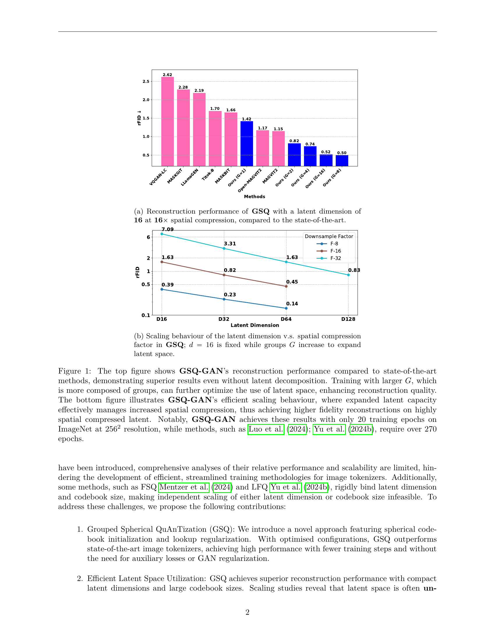
🔼 This figure shows a bar chart comparing the reconstruction performance (measured by FID score) of the proposed GSQ method with a latent dimension of 16 and 16x spatial compression against several state-of-the-art image reconstruction methods. Lower FID indicates better reconstruction quality. GSQ demonstrates superior reconstruction quality compared to other methods.
read the caption
(a) Reconstruction performance of GSQ with a latent dimension of 16 at 16×\times× spatial compression, compared to the state-of-the-art.
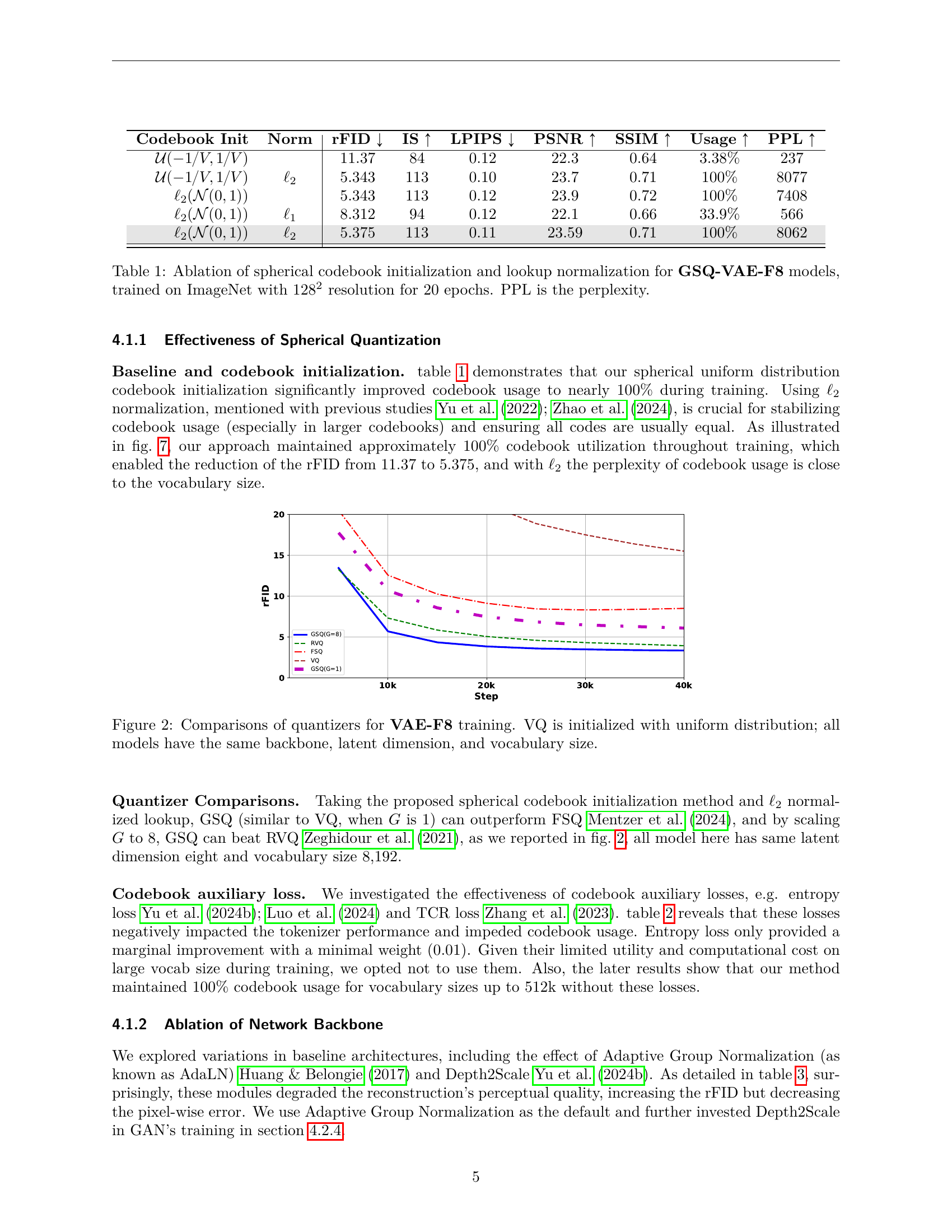
| Codebook Init | Norm | rFID ↓ | IS ↑ | LPIPS ↓ | PSNR ↑ | SSIM ↑ | Usage ↑ | PPL ↑ |
|---|---|---|---|---|---|---|---|---|
| \mathcal{U}(-1/V,1/V) | 11.37 | 84 | 0.12 | 22.3 | 0.64 | 3.38% | 237 | |
| \mathcal{U}(-1/V,1/V) | \ell_{2} | 5.343 | 113 | 0.10 | 23.7 | 0.71 | 100% | 8077 |
| \ell_{2}(\mathcal{N}(0,1)) | 5.343 | 113 | 0.12 | 23.9 | 0.72 | 100% | 7408 | |
| \ell_{2}(\mathcal{N}(0,1)) | \ell_{1} | 8.312 | 94 | 0.12 | 22.1 | 0.66 | 33.9% | 566 |
| \ell_{2}(\mathcal{N}(0,1)) | \ell_{2} | 5.375 | 113 | 0.11 | 23.59 | 0.71 | 100% | 8062 |
🔼 This table presents an ablation study on the effects of spherical codebook initialization and l2-lookup normalization in the Grouped Spherical Quantization (GSQ) Variational Autoencoder (VAE) model. The experiments were conducted on the ImageNet dataset at a resolution of 128x128, with training for 20 epochs. Different codebook initialization methods (uniform distribution within a range [-1/V, 1/V] and a spherical uniform distribution l2(N(0,1))) and lookup normalization techniques (l1 and l2) are compared. The table shows the impact of these choices on reconstruction performance metrics (rFID, IS, LPIPS, PSNR, SSIM, and Usage), and model perplexity (PPL). The results highlight the significant improvements achieved by using spherical codebook initialization and l2 normalization.
read the caption
Table 1: Ablation of spherical codebook initialization and lookup normalization for GSQ-VAE-F8 models, trained on ImageNet with 1282superscript1282128^{2}128 start_POSTSUPERSCRIPT 2 end_POSTSUPERSCRIPT resolution for 20 epochs. PPL is the perplexity.
In-depth insights#
GSQ: Spherical Edge#
The heading ‘GSQ: Spherical Edge’ suggests a novel approach to image tokenization, building upon Grouped Spherical Quantization (GSQ). A key innovation might be the integration of spherical geometry principles at the edges of image patches or tokens. This could improve the representation of boundaries and object contours. Improved boundary handling is crucial for image reconstruction and generation, especially at high compression ratios. The ‘spherical edge’ concept potentially addresses limitations of traditional quantization methods that struggle with sharp transitions, resulting in artifacts or blurriness near edges. A key aspect to investigate would be how this spherical edge treatment impacts the overall reconstruction quality, especially compared to standard methods. It’s possible this approach enhances the network’s ability to capture high-frequency information and fine details in images. The effectiveness would likely depend on the choice of distance metric and the implementation details of the ‘spherical edge’ itself, including its interaction with the core GSQ algorithm. Further analysis of computational cost and memory requirements is also important. The overall goal of this innovation would be to improve reconstruction fidelity and achieve superior compression performance in image tokenization tasks.
VQ-GAN Scaling Laws#
Investigating VQ-GAN scaling laws would involve exploring how key model parameters like latent dimension, codebook size, and spatial compression ratio affect performance metrics such as reconstruction quality (e.g., FID score) and training efficiency. A crucial aspect would be identifying optimal scaling strategies: does increasing latent dimensionality always improve results, or is there a point of diminishing returns? Similarly, how does codebook size interact with latent dimension? Understanding the interplay between these factors is key to efficiently scaling VQ-GANs for higher-resolution images and improved generative quality. The analysis should consider computational costs as well, assessing the trade-offs between increased performance and increased resource requirements. Ideally, a comprehensive study would formulate scaling laws that predict performance based on these parameters, offering practical guidelines for efficient model design and training at various scales.
GSQ-GAN Ablation#
A hypothetical ‘GSQ-GAN Ablation’ section would systematically evaluate the impact of individual components within the GSQ-GAN architecture. This would involve controlled experiments, modifying one aspect (e.g., the type of quantizer, loss function, or network architecture) while holding others constant. The results would reveal the contribution of each component to the overall model performance, measured by metrics like FID (Fréchet Inception Distance) and reconstruction quality. Key insights would include identifying crucial components for optimal performance, potentially suggesting areas for improvement or simplification of the model. For example, ablation might show that a specific loss function is essential for high-quality reconstruction, or that a certain network architecture is more efficient while maintaining accuracy. Ultimately, the ablation study helps establish a clear understanding of GSQ-GAN’s strengths and weaknesses, guiding future model development and optimization.
Latent Space Scaling#
The concept of ‘Latent Space Scaling’ in the context of image tokenizers is crucial for achieving efficiency and high-quality reconstruction. The paper investigates how increasing latent dimensionality and codebook size affects performance. Crucially, it finds that simply increasing latent dimensions does not always translate to better results, highlighting the challenges of high-dimensional spaces. The authors propose Grouped Spherical Quantization (GSQ), a method for structuring latent space to efficiently manage high dimensionality. GSQ demonstrably enables better scaling with improved reconstruction quality at higher compression ratios, outperforming existing methods. The study’s findings strongly suggest that carefully considered latent space organization, particularly via techniques like GSQ, is paramount for building scalable and effective image tokenizers. The optimal balance between latent dimensionality and codebook size is a key finding, suggesting future research should focus on adaptive strategies to dynamically optimize these parameters based on task-specific needs.
Future: High-res GANs#
The prospect of “Future: High-res GANs” is exciting, suggesting advancements in generating high-resolution images with Generative Adversarial Networks. Current limitations in high-resolution image generation using GANs include computational cost and training instability. Future work likely involves exploring new architectures, optimized training methods (perhaps incorporating techniques from other generative models), and more sophisticated loss functions to improve image quality and efficiency. Efficient latent space utilization and novel quantization techniques, as explored in the provided paper, are essential aspects of this high-res GAN future. Research into more stable and robust training processes is crucial for successful upscaling, potentially through enhanced regularization methods or alternative training strategies. Ultimately, a successful “High-res GANs” future relies on addressing computational bottlenecks and resolving training instability while ensuring superior image fidelity compared to existing models.
More visual insights#
More on figures

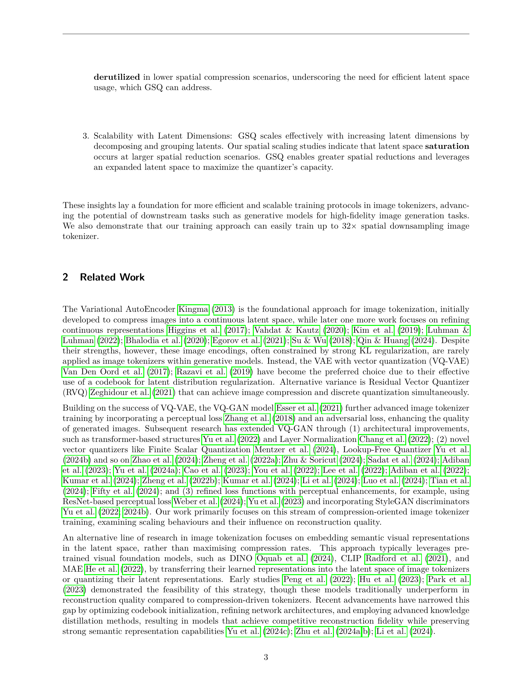
🔼 This figure shows how the model scales with the latent dimension and spatial compression factor. The latent dimension (d) is held constant at 16, while the number of groups (G), which control the latent space expansion, is varied. The x-axis represents the latent dimension, while the y-axis shows the spatial compression factor. The plot illustrates the relationship between the latent dimension, the number of groups, and the spatial compression achieved by the model.
read the caption
(b) Scaling behaviour of the latent dimension v.s. spatial compression factor in GSQ; d=16𝑑16d=16italic_d = 16 is fixed while groups G𝐺Gitalic_G increase to expand latent space.

🔼 Figure 1 demonstrates GSQ-GAN’s superior image reconstruction capabilities compared to other state-of-the-art methods. The top panel shows that GSQ-GAN achieves a lower reconstruction FID (Frechet Inception Distance) score, indicating better reconstruction quality, even without employing latent decomposition techniques. Increasing the number of groups (G) during training further improves performance by optimizing the use of latent space. The bottom panel illustrates GSQ-GAN’s scalability. It shows that by increasing the latent capacity, GSQ-GAN maintains high-fidelity reconstruction even at high spatial compression ratios (16x downsampling in this case). This is achieved using significantly fewer training epochs (20) compared to existing methods (over 270 epochs).
read the caption
Figure 1: The top figure shows GSQ-GAN’s reconstruction performance compared to state-of-the-art methods, demonstrating superior results even without latent decomposition. Training with larger G𝐺Gitalic_G, which is more composed of groups, can further optimize the use of latent space, enhancing reconstruction quality. The bottom figure illustrates GSQ-GAN’s efficient scaling behaviour, where expanded latent capacity effectively manages increased spatial compression, thus achieving higher fidelity reconstructions on highly spatial compressed latent. Notably, GSQ-GAN achieves these results with only 20 training epochs on ImageNet at 2562superscript2562256^{2}256 start_POSTSUPERSCRIPT 2 end_POSTSUPERSCRIPT resolution, while methods, such as Luo et al. (2024); Yu et al. (2024b), require over 270 epochs.

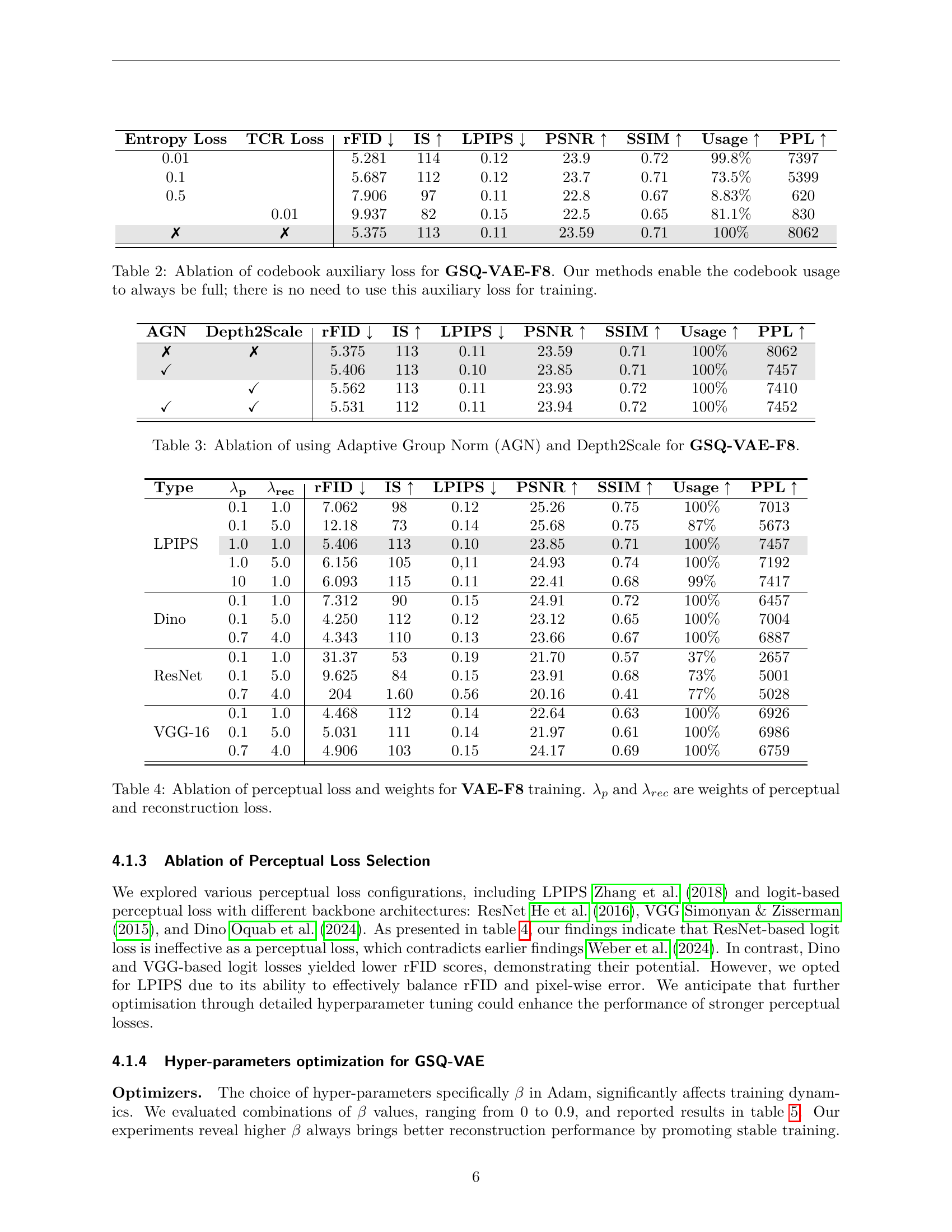
🔼 This figure compares the performance of different vector quantization (VQ) methods for training a variational autoencoder (VAE) on images with an 8x spatial compression factor. The methods compared are VQ (Vector Quantization), RVQ (Residual Vector Quantization), FSQ (Finite Scalar Quantization), and the proposed GSQ (Grouped Spherical Quantization). All methods use the same VAE architecture (backbone), latent dimension, and codebook size, ensuring a fair comparison. The graph shows the reconstruction error (rFID) over training steps, illustrating the relative efficiency and effectiveness of each quantization technique. The key difference lies in how the latent vectors are quantized to discrete codebook indices, impacting the quality of the reconstructed images.
read the caption
Figure 2: Comparisons of quantizers for VAE-F8 training. VQ is initialized with uniform distribution; all models have the same backbone, latent dimension, and vocabulary size.

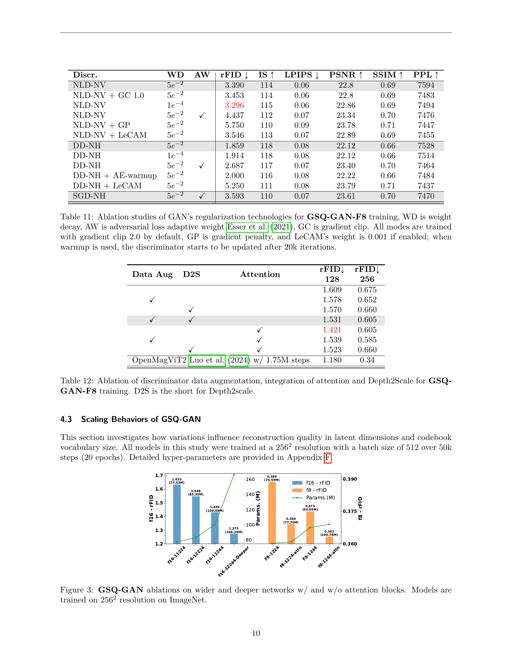
🔼 This figure displays the ablation study results of GSQ-GAN model trained on ImageNet with 256x256 resolution images. It shows the impact of increasing network width and depth, with and without attention blocks, on the model’s reconstruction performance. The results demonstrate that wider and deeper networks, especially those with attention blocks, lead to better reconstruction quality. The x-axis likely represents a measure of network complexity (e.g., number of parameters), and the y-axis shows reconstruction error.
read the caption
Figure 3: GSQ-GAN ablations on wider and deeper networks w/ and w/o attention blocks. Models are trained on 2562superscript2562256^{2}256 start_POSTSUPERSCRIPT 2 end_POSTSUPERSCRIPT resolution on ImageNet.

🔼 This figure shows how the reconstruction quality of the GSQ model changes when varying the latent dimension and vocabulary size at 8x spatial compression. The x-axis represents the latent dimension, while the y-axis shows the reconstruction error (rFID). Multiple lines are plotted, each corresponding to different vocabulary sizes. The figure helps in understanding the impact of increasing latent dimension and vocabulary size on the model’s performance during the compression process. It helps to determine the optimal combination of latent dimension and vocabulary size for a given compression ratio.
read the caption
(a) Scaling of latent dimension and vocabulary size for GSQ at 8×\times× spatial compression.

🔼 Figure 4b shows the relationship between reconstruction quality (rFID), latent dimension, and codebook size. The x-axis represents the codebook size (vocabulary) on a logarithmic scale, and the y-axis represents rFID. Different lines represent different latent dimensions. The figure demonstrates that increasing codebook size generally improves reconstruction quality (lower rFID), and that the optimal codebook size may depend on the latent dimension.
read the caption
(b) Same scaling behaviour as the top figure with vocabulary size in logarithmic scale.

🔼 This figure analyzes the impact of latent dimension and codebook size on the reconstruction quality of the GSQ image tokenizer at 8x spatial compression. The top panel shows that smaller latent dimensions lead to better reconstruction, indicating the latent space is not fully utilized at this compression level. Increasing the codebook size further improves performance. The bottom panel presents the same data but with the vocabulary size shown on a logarithmic scale, highlighting the effectiveness of scaling the codebook size. Importantly, all models in this experiment were trained using G=1, meaning there was no latent space decomposition, making them directly comparable to traditional VQ-based methods. The training dataset used was ImageNet with images of 256x256 resolution.
read the caption
Figure 4: The top figure illustrates the scaling of latent dimension and codebook size for GSQ at 8×\times× spatial compression, where a smaller latent dimension improves reconstruction, suggesting the latent space is not saturated for F8 downsampling. Optimising latent space size further enhances performance. The bottom figure shows the same trend with vocabulary size in logarithmic scale, indicating effective scaling as vocabulary size increases. All models are trained with G=1𝐺1G=1italic_G = 1 and no latent decomposition, making this equivalent to VQ-based methods. All models are trained on ImageNet at 2562superscript2562256^{2}256 start_POSTSUPERSCRIPT 2 end_POSTSUPERSCRIPT resolution.

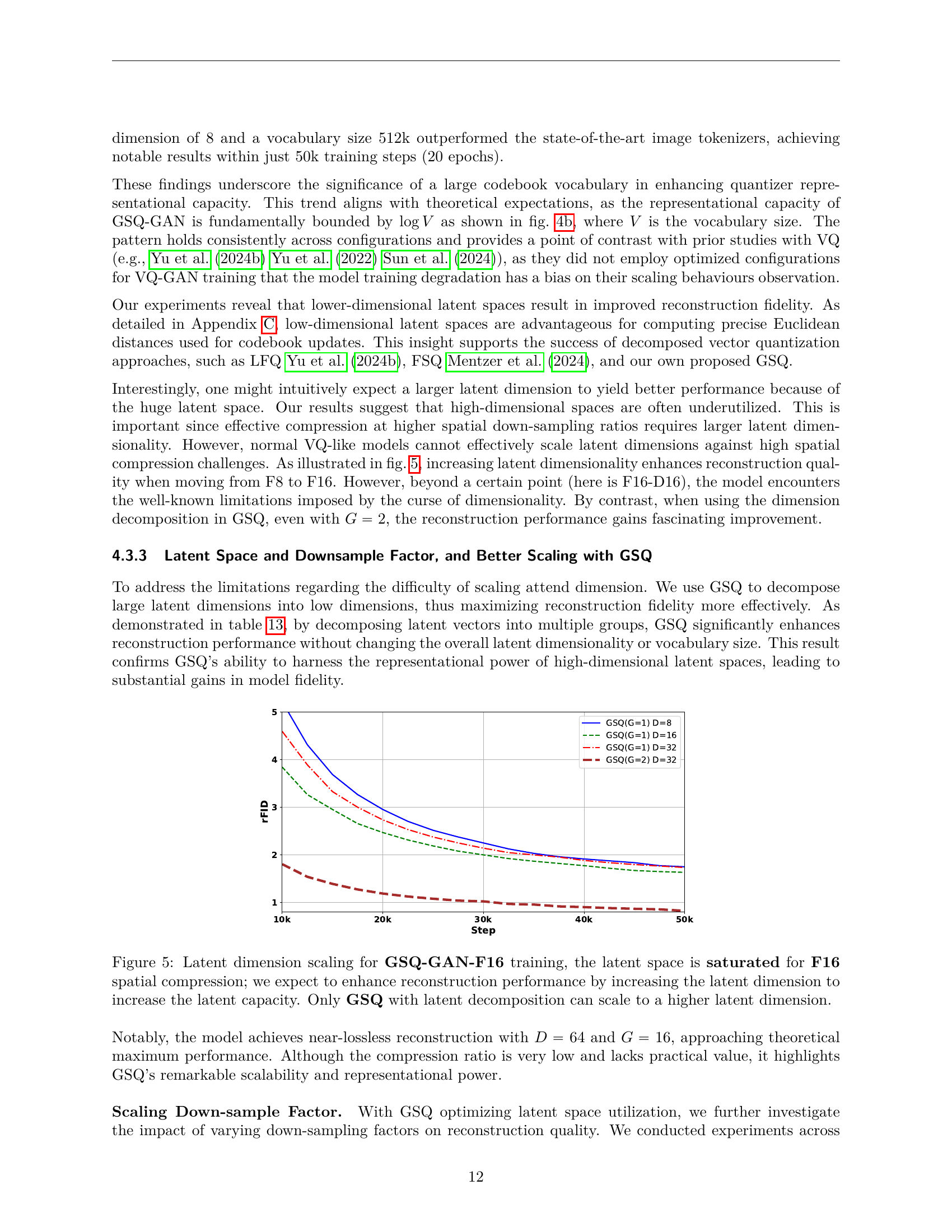
🔼 Figure 5 demonstrates the effect of increasing latent dimensionality on the reconstruction performance of GSQ-GAN when the spatial compression ratio is 16 (F16). The figure shows that increasing the latent dimension initially improves reconstruction quality, but beyond a certain point (D=16 in this case), adding more dimensions does not provide further gains. This saturation effect highlights the limitations of standard VQ techniques in high-dimensional latent spaces. However, GSQ with latent decomposition (using multiple groups, G >1) successfully scales to much higher latent dimensions (32 and 64) and continues to show significant improvements in reconstruction performance. This highlights the effectiveness of GSQ in managing the complexity of high-dimensional spaces, resulting in improved image generation quality.
read the caption
Figure 5: Latent dimension scaling for GSQ-GAN-F16 training, the latent space is saturated for F16 spatial compression; we expect to enhance reconstruction performance by increasing the latent dimension to increase the latent capacity. Only GSQ with latent decomposition can scale to a higher latent dimension.
More on tables
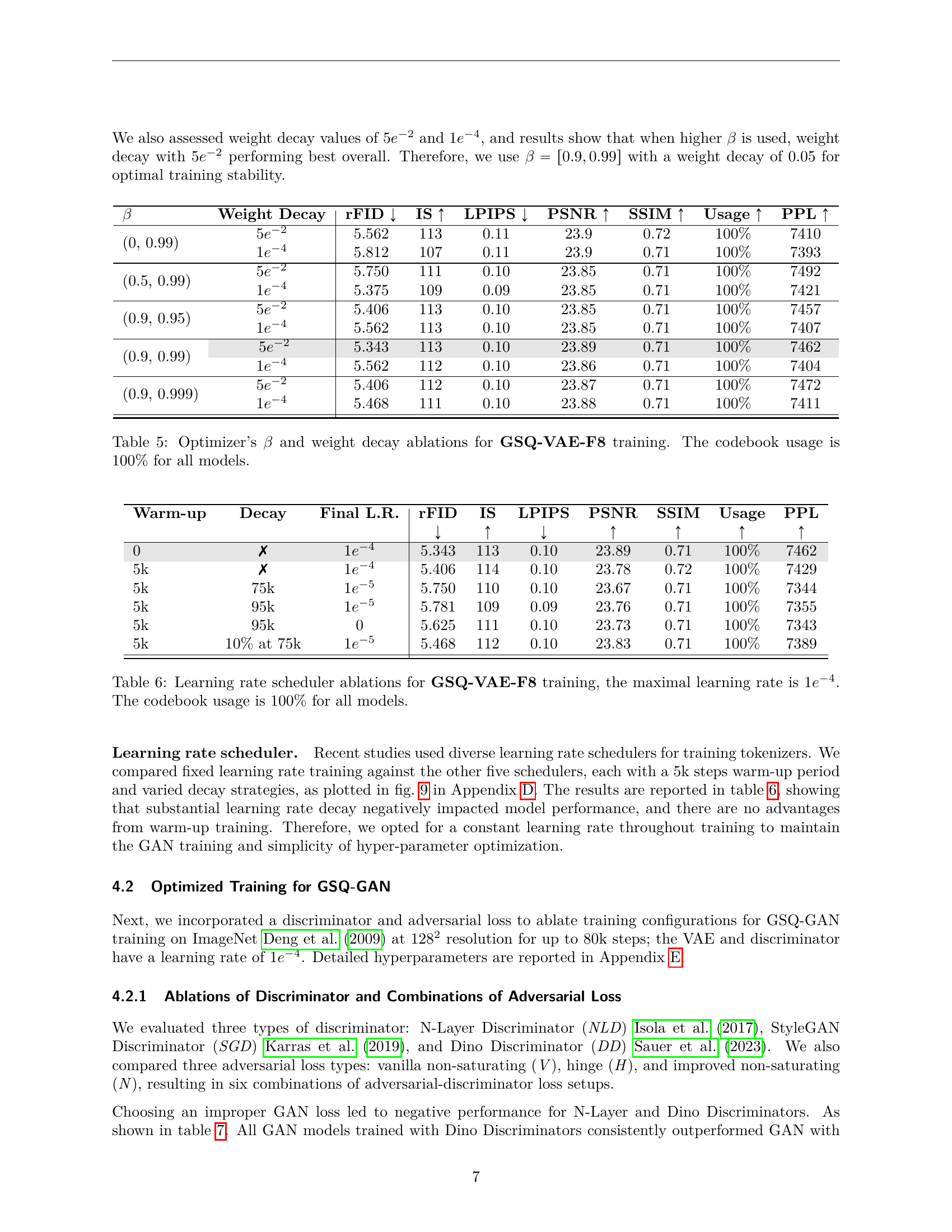
| Entropy Loss | TCR Loss | rFID ↓ | IS ↑ | LPIPS ↓ | PSNR ↑ | SSIM ↑ | Usage ↑ | PPL ↑ |
|---|---|---|---|---|---|---|---|---|
| 0.01 | 5.281 | 114 | 0.12 | 23.9 | 0.72 | 99.8% | 7397 | |
| 0.1 | 5.687 | 112 | 0.12 | 23.7 | 0.71 | 73.5% | 5399 | |
| 0.5 | 7.906 | 97 | 0.11 | 22.8 | 0.67 | 8.83% | 620 | |
| 0.01 | 9.937 | 82 | 0.15 | 22.5 | 0.65 | 81.1% | 830 | |
| ✗ | ✗ | 5.375 | 113 | 0.11 | 23.59 | 0.71 | 100% | 8062 |
🔼 This table presents an ablation study on the impact of codebook auxiliary loss functions (entropy and TCR loss) on the performance of the GSQ-VAE-F8 model. The results show that adding these auxiliary loss functions does not improve performance and even negatively impacts codebook utilization. The GSQ-VAE-F8 model, with the proposed spherical quantization method, consistently achieves near-full codebook usage (close to 100%) without the need for any auxiliary loss. This demonstrates the effectiveness of the proposed GSQ method.
read the caption
Table 2: Ablation of codebook auxiliary loss for GSQ-VAE-F8. Our methods enable the codebook usage to always be full; there is no need to use this auxiliary loss for training.
| AGN | Depth2Scale | rFID ↓ | IS ↑ | LPIPS ↓ | PSNR ↑ | SSIM ↑ | Usage ↑ | PPL ↑ |
|---|---|---|---|---|---|---|---|---|
| ✗ | ✗ | 5.375 | 113 | 0.11 | 23.59 | 0.71 | 100% | 8062 |
| ✓ | 5.406 | 113 | 0.10 | 23.85 | 0.71 | 100% | 7457 | |
| ✓ | 5.562 | 113 | 0.11 | 23.93 | 0.72 | 100% | 7410 | |
| ✓ | ✓ | 5.531 | 112 | 0.11 | 23.94 | 0.72 | 100% | 7452 |
🔼 This table presents the ablation study results on the impact of using Adaptive Group Normalization (AGN) and Depth2Scale modules within the GSQ-VAE-F8 model. It shows how the reconstruction performance (rFID), Inception Score (IS), Learned Perceptual Image Patch Similarity (LPIPS), Peak Signal-to-Noise Ratio (PSNR), Structural Similarity Index (SSIM), codebook usage, and perplexity (PPL) change when AGN and/or Depth2Scale is included or excluded. This helps to understand the contribution of each module to the overall performance of the image tokenizer model.
read the caption
Table 3: Ablation of using Adaptive Group Norm (AGN) and Depth2Scale for GSQ-VAE-F8.
| Type | λp | λrec | rFID ↓ | IS ↑ | LPIPS ↓ | PSNR ↑ | SSIM ↑ | Usage ↑ | PPL ↑ |
|---|---|---|---|---|---|---|---|---|---|
| LPIPS | 0.1 | 1.0 | 7.062 | 98 | 0.12 | 25.26 | 0.75 | 100% | 7013 |
| 0.1 | 5.0 | 12.18 | 73 | 0.14 | 25.68 | 0.75 | 87% | 5673 | |
| 1.0 | 1.0 | 5.406 | 113 | 0.10 | 23.85 | 0.71 | 100% | 7457 | |
| 1.0 | 5.0 | 6.156 | 105 | 0.11 | 24.93 | 0.74 | 100% | 7192 | |
| 10 | 1.0 | 6.093 | 115 | 0.11 | 22.41 | 0.68 | 99% | 7417 | |
| Dino | 0.1 | 1.0 | 7.312 | 90 | 0.15 | 24.91 | 0.72 | 100% | 6457 |
| 0.1 | 5.0 | 4.250 | 112 | 0.12 | 23.12 | 0.65 | 100% | 7004 | |
| 0.7 | 4.0 | 4.343 | 110 | 0.13 | 23.66 | 0.67 | 100% | 6887 | |
| ResNet | 0.1 | 1.0 | 31.37 | 53 | 0.19 | 21.70 | 0.57 | 37% | 2657 |
| 0.1 | 5.0 | 9.625 | 84 | 0.15 | 23.91 | 0.68 | 73% | 5001 | |
| 0.7 | 4.0 | 204 | 1.60 | 0.56 | 20.16 | 0.41 | 77% | 5028 | |
| VGG-16 | 0.1 | 1.0 | 4.468 | 112 | 0.14 | 22.64 | 0.63 | 100% | 6926 |
| 0.1 | 5.0 | 5.031 | 111 | 0.14 | 21.97 | 0.61 | 100% | 6986 | |
| 0.7 | 4.0 | 4.906 | 103 | 0.15 | 24.17 | 0.69 | 100% | 6759 |
🔼 This table presents an ablation study on the impact of different perceptual loss functions and their associated weights on the performance of a VAE model (specifically, the VAE-F8 model, as indicated by the table’s title) during training. It examines different configurations by varying weights assigned to perceptual loss (λp) and reconstruction loss (λrec). The results likely show how the balance between these two loss types affects the model’s ability to reconstruct images accurately and maintain perceptual fidelity (i.e., how well the reconstructed images resemble the original images visually). The table likely shows various metrics evaluating reconstruction quality.
read the caption
Table 4: Ablation of perceptual loss and weights for VAE-F8 training. λpsubscript𝜆𝑝\lambda_{p}italic_λ start_POSTSUBSCRIPT italic_p end_POSTSUBSCRIPT and λrecsubscript𝜆𝑟𝑒𝑐\lambda_{rec}italic_λ start_POSTSUBSCRIPT italic_r italic_e italic_c end_POSTSUBSCRIPT are weights of perceptual and reconstruction loss.
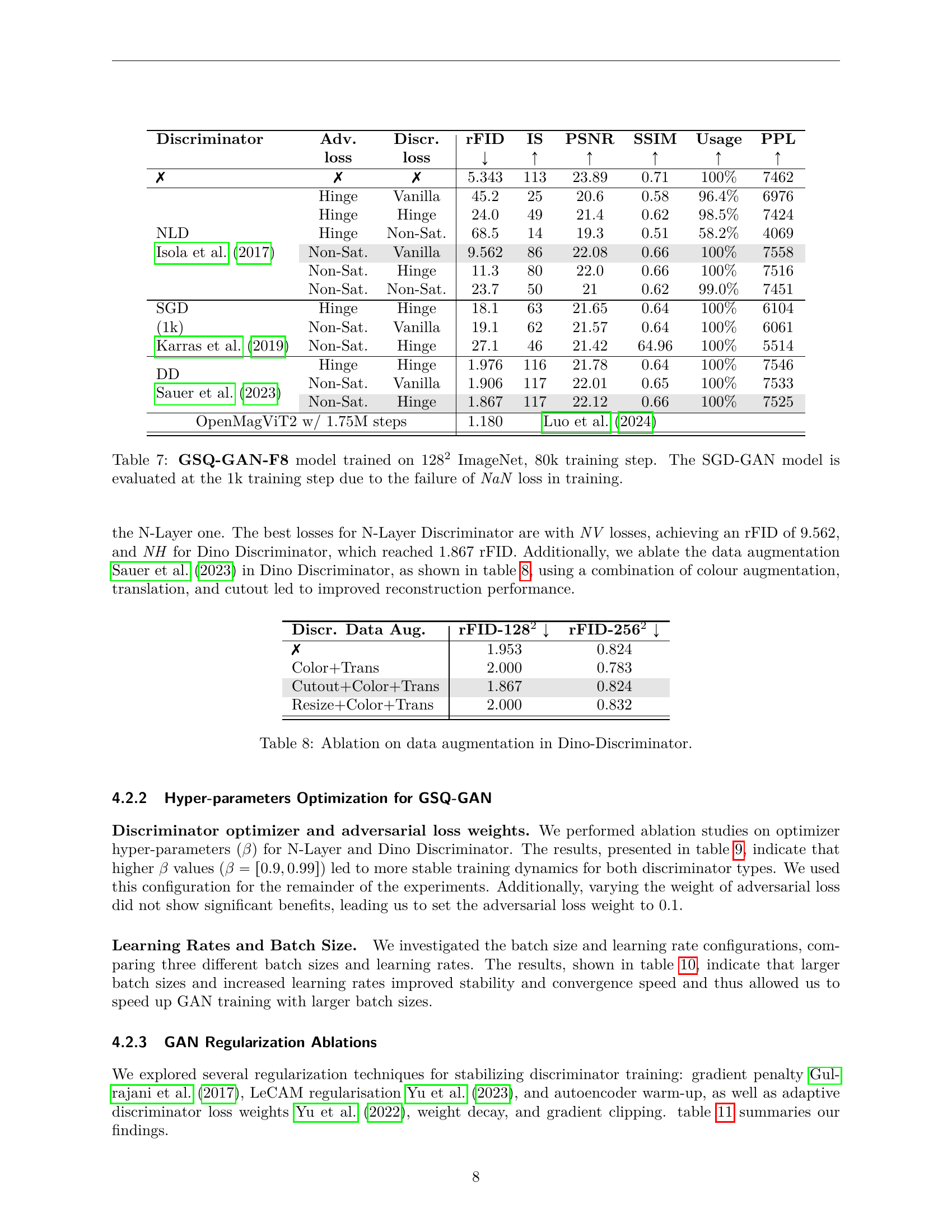
| β | Weight Decay | rFID ↓ | IS ↑ | LPIPS ↓ | PSNR ↑ | SSIM ↑ | Usage ↑ | PPL ↑ |
|---|---|---|---|---|---|---|---|---|
| (0, 0.99) | 5e⁻² | 5.562 | 113 | 0.11 | 23.9 | 0.72 | 100% | 7410 |
| 1e⁻⁴ | 5.812 | 107 | 0.11 | 23.9 | 0.71 | 100% | 7393 | |
| (0.5, 0.99) | 5e⁻² | 5.750 | 111 | 0.10 | 23.85 | 0.71 | 100% | 7492 |
| 1e⁻⁴ | 5.375 | 109 | 0.09 | 23.85 | 0.71 | 100% | 7421 | |
| (0.9, 0.95) | 5e⁻² | 5.406 | 113 | 0.10 | 23.85 | 0.71 | 100% | 7457 |
| 1e⁻⁴ | 5.562 | 113 | 0.10 | 23.85 | 0.71 | 100% | 7407 | |
| (0.9, 0.99) | 5e⁻² | 5.343 | 113 | 0.10 | 23.89 | 0.71 | 100% | 7462 |
| 1e⁻⁴ | 5.562 | 112 | 0.10 | 23.86 | 0.71 | 100% | 7404 | |
| (0.9, 0.999) | 5e⁻² | 5.406 | 112 | 0.10 | 23.87 | 0.71 | 100% | 7472 |
| 1e⁻⁴ | 5.468 | 111 | 0.10 | 23.88 | 0.71 | 100% | 7411 |
🔼 This table presents the results of ablation studies on the hyperparameters of the Adam optimizer used for training the GSQ-VAE-F8 model. Specifically, it investigates the impact of different beta values (β1 and β2) and weight decay on the model’s performance. The table shows the reconstruction performance metrics (rFID, IS, LPIPS, PSNR, SSIM, Usage, and PPL) achieved using various combinations of beta values and weight decay. A key observation is that the codebook usage remains at 100% across all configurations tested, indicating that the chosen hyperparameters effectively utilize the entire codebook.
read the caption
Table 5: Optimizer’s β𝛽\betaitalic_β and weight decay ablations for GSQ-VAE-F8 training. The codebook usage is 100% for all models.
| Warm-up | Decay | Final L.R. | rFID | IS | LPIPS | PSNR | SSIM | Usage | PPL |
|---|---|---|---|---|---|---|---|---|---|
| 0 | ✗ | 1e⁻⁴ | 5.343 | 113 | 0.10 | 23.89 | 0.71 | 100% | 7462 |
| 5k | ✗ | 1e⁻⁴ | 5.406 | 114 | 0.10 | 23.78 | 0.72 | 100% | 7429 |
| 5k | 75k | 1e⁻⁵ | 5.750 | 110 | 0.10 | 23.67 | 0.71 | 100% | 7344 |
| 5k | 95k | 1e⁻⁵ | 5.781 | 109 | 0.09 | 23.76 | 0.71 | 100% | 7355 |
| 5k | 95k | 0 | 5.625 | 111 | 0.10 | 23.73 | 0.71 | 100% | 7343 |
| 5k | 10% at 75k | 1e⁻⁵ | 5.468 | 112 | 0.10 | 23.83 | 0.71 | 100% | 7389 |
🔼 This table presents an ablation study on different learning rate schedulers used during the training of a Variational Autoencoder (VAE) for image tokenization. The goal is to determine the optimal learning rate schedule for achieving high-quality image reconstruction. Several schedules are compared, including those with and without a warm-up period and with different decay rates. The table shows the impact of each schedule on the reconstruction fidelity (rFID), Inception Score (IS), LPIPS, PSNR, SSIM, codebook usage, and perplexity (PPL). The maximal learning rate used across all experiments was 1e-4. The experiment shows that a constant learning rate provides the best performance, highlighting the tradeoffs between fast convergence and model quality.
read the caption
Table 6: Learning rate scheduler ablations for GSQ-VAE-F8 training, the maximal learning rate is 1e−4superscript𝑒4e^{-4}italic_e start_POSTSUPERSCRIPT - 4 end_POSTSUPERSCRIPT. The codebook usage is 100% for all models.
| Discriminator | Adv. loss | Discr. loss | rFID | IS | PSNR | SSIM | Usage | PPL |
|---|---|---|---|---|---|---|---|---|
| loss | loss | ↓ | ↑ | ↑ | ↑ | ↑ | ↑ | |
| ✗ | ✗ | ✗ | 5.343 | 113 | 23.89 | 0.71 | 100% | 7462 |
| NLD Isola et al. (2017) | Hinge | Vanilla | 45.2 | 25 | 20.6 | 0.58 | 96.4% | 6976 |
| Hinge | Hinge | 24.0 | 49 | 21.4 | 0.62 | 98.5% | 7424 | |
| Hinge | Non-Sat. | 68.5 | 14 | 19.3 | 0.51 | 58.2% | 4069 | |
| Non-Sat. | Vanilla | 9.562 | 86 | 22.08 | 0.66 | 100% | 7558 | |
| Non-Sat. | Hinge | 11.3 | 80 | 22.0 | 0.66 | 100% | 7516 | |
| Non-Sat. | Non-Sat. | 23.7 | 50 | 21 | 0.62 | 99.0% | 7451 | |
| SGD (1k) Karras et al. (2019) | Hinge | Hinge | 18.1 | 63 | 21.65 | 0.64 | 100% | 6104 |
| Non-Sat. | Vanilla | 19.1 | 62 | 21.57 | 0.64 | 100% | 6061 | |
| Non-Sat. | Hinge | 27.1 | 46 | 21.42 | 64.96 | 100% | 5514 | |
| DD Sauer et al. (2023) | Hinge | Hinge | 1.976 | 116 | 21.78 | 0.64 | 100% | 7546 |
| Non-Sat. | Vanilla | 1.906 | 117 | 22.01 | 0.65 | 100% | 7533 | |
| Non-Sat. | Hinge | 1.867 | 117 | 22.12 | 0.66 | 100% | 7525 | |
| OpenMagViT2 w/ 1.75M steps | 1.180 | Luo et al. (2024) |
🔼 This table presents the results of training a GSQ-GAN (Grouped Spherical Quantization Generative Adversarial Network) model on the ImageNet dataset at a resolution of 128x128 pixels. The training involved 80,000 steps, except for the StyleGAN model which was stopped after 1000 steps due to NaN losses during training. The table compares the reconstruction performance (rFID), Inception Score (IS), Peak Signal-to-Noise Ratio (PSNR), Structural Similarity Index (SSIM), Codebook Usage, and Perplexity (PPL) across different discriminator architectures (NLD, SGD, DD) and adversarial loss functions (Vanilla, Hinge, Non-Saturating). This allows for a comprehensive analysis of various components and configurations within the GSQ-GAN model and their effect on performance.
read the caption
Table 7: GSQ-GAN-F8 model trained on 1282 ImageNet, 80k training step. The SGD-GAN model is evaluated at the 1k training step due to the failure of 𝑁𝑎𝑁𝑁𝑎𝑁\mathit{NaN}italic_NaN loss in training.
| Discr. Data Aug. | rFID-128 ↓ | rFID-256 ↓ |
|---|---|---|
| ✗ | 1.953 | 0.824 |
| Color+Trans | 2.000 | 0.783 |
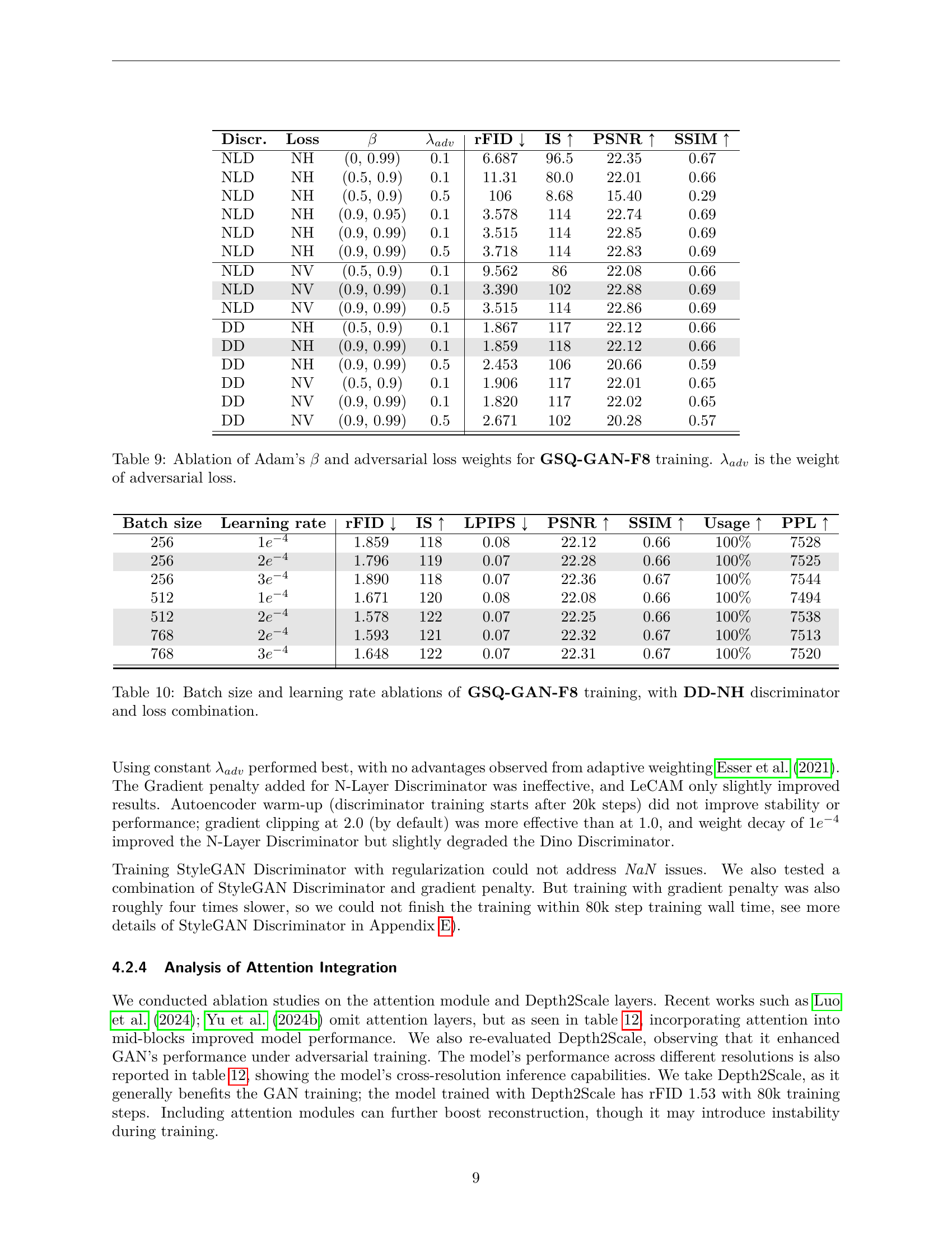
| Cutout+Color+Trans | 1.867 | 0.824 |
| Resize+Color+Trans | 2.000 | 0.832 |
🔼 This table presents the ablation study on different data augmentation techniques used in the Dino-Discriminator within the GSQ-GAN model. It shows the impact of color augmentation, translation, and cutout on the reconstruction performance (measured by rFID) at two different spatial resolutions: 128x128 and 256x256.
read the caption
Table 8: Ablation on data augmentation in Dino-Discriminator.
| Discr. | Loss | β | λadv | rFID ↓ | IS ↑ | PSNR ↑ | SSIM ↑ |
|---|---|---|---|---|---|---|---|
| NLD | NH | (0, 0.99) | 0.1 | 6.687 | 96.5 | 22.35 | 0.67 |
| NLD | NH | (0.5, 0.9) | 0.1 | 11.31 | 80.0 | 22.01 | 0.66 |
| NLD | NH | (0.5, 0.9) | 0.5 | 106 | 8.68 | 15.40 | 0.29 |
| NLD | NH | (0.9, 0.95) | 0.1 | 3.578 | 114 | 22.74 | 0.69 |
| NLD | NH | (0.9, 0.99) | 0.1 | 3.515 | 114 | 22.85 | 0.69 |
| NLD | NH | (0.9, 0.99) | 0.5 | 3.718 | 114 | 22.83 | 0.69 |
| NLD | NV | (0.5, 0.9) | 0.1 | 9.562 | 86 | 22.08 | 0.66 |
| NLD | NV | (0.9, 0.99) | 0.1 | 3.390 | 102 | 22.88 | 0.69 |
| NLD | NV | (0.9, 0.99) | 0.5 | 3.515 | 114 | 22.86 | 0.69 |
| DD | NH | (0.5, 0.9) | 0.1 | 1.867 | 117 | 22.12 | 0.66 |
| DD | NH | (0.9, 0.99) | 0.1 | 1.859 | 118 | 22.12 | 0.66 |
| DD | NH | (0.9, 0.99) | 0.5 | 2.453 | 106 | 20.66 | 0.59 |
| DD | NV | (0.5, 0.9) | 0.1 | 1.906 | 117 | 22.01 | 0.65 |
| DD | NV | (0.9, 0.99) | 0.1 | 1.820 | 117 | 22.02 | 0.65 |
| DD | NV | (0.9, 0.99) | 0.5 | 2.671 | 102 | 20.28 | 0.57 |
🔼 This table presents the results of ablation studies on the hyperparameters of the Adam optimizer and the weight of the adversarial loss in the GSQ-GAN-F8 model training. It shows how different values of Adam’s beta parameters (β1 and β2) and the adversarial loss weight (λadv) affect the model’s performance, as measured by the FID (Fréchet Inception Distance) score. The table helps to determine the optimal hyperparameter settings for training the GSQ-GAN-F8 model.
read the caption
Table 9: Ablation of Adam’s β𝛽\betaitalic_β and adversarial loss weights for GSQ-GAN-F8 training. λadvsubscript𝜆𝑎𝑑𝑣\lambda_{adv}italic_λ start_POSTSUBSCRIPT italic_a italic_d italic_v end_POSTSUBSCRIPT is the weight of adversarial loss.
| Batch size | Learning rate | rFID ↓ | IS ↑ | LPIPS ↓ | PSNR ↑ | SSIM ↑ | Usage ↑ | PPL ↑ |
|---|---|---|---|---|---|---|---|---|
| 256 | 1e⁻⁴ | 1.859 | 118 | 0.08 | 22.12 | 0.66 | 100% | 7528 |
| 256 | 2e⁻⁴ | 1.796 | 119 | 0.07 | 22.28 | 0.66 | 100% | 7525 |
| 256 | 3e⁻⁴ | 1.890 | 118 | 0.07 | 22.36 | 0.67 | 100% | 7544 |
| 512 | 1e⁻⁴ | 1.671 | 120 | 0.08 | 22.08 | 0.66 | 100% | 7494 |
| 512 | 2e⁻⁴ | 1.578 | 122 | 0.07 | 22.25 | 0.66 | 100% | 7538 |
| 768 | 2e⁻⁴ | 1.593 | 121 | 0.07 | 22.32 | 0.67 | 100% | 7513 |
| 768 | 3e⁻⁴ | 1.648 | 122 | 0.07 | 22.31 | 0.67 | 100% | 7520 |
🔼 This table presents the results of ablation studies on the batch size and learning rate used during the training of the GSQ-GAN-F8 model. The experiment varied the batch size (256, 512, 768) and learning rate (1e-4, 2e-4, 3e-4) to determine their impact on the model’s performance. The performance is measured by rFID (Reconstruction Fidelity), Inception Score (IS), LPIPS (Learned Perceptual Image Patch Similarity), PSNR (Peak Signal-to-Noise Ratio), SSIM (Structural Similarity Index), Codebook Usage, and Perplexity (PPL). The Dino Discriminator (DD) and the Hinge-NonSaturating (NH) loss combination were used consistently in this experiment.
read the caption
Table 10: Batch size and learning rate ablations of GSQ-GAN-F8 training, with DD-NH discriminator and loss combination.
| Discr. | WD | AW | rFID ↓ | IS ↑ | LPIPS ↓ | PSNR ↑ | SSIM ↑ | PPL ↑ |
|---|---|---|---|---|---|---|---|---|
| NLD-NV | 5e-2 | 3.390 | 114 | 0.06 | 22.8 | 0.69 | 7594 | |
| NLD-NV + GC 1.0 | 5e-2 | 3.453 | 114 | 0.06 | 22.8 | 0.69 | 7483 | |
| NLD-NV | 1e-4 | 3.296 | 115 | 0.06 | 22.86 | 0.69 | 7494 | |
| NLD-NV | 5e-2 | ✓ | 4.437 | 112 | 0.07 | 23.34 | 0.70 | 7476 |
| NLD-NV + GP | 5e-2 | 5.750 | 110 | 0.09 | 23.78 | 0.71 | 7447 | |
| NLD-NV + LeCAM | 5e-2 | 3.546 | 113 | 0.07 | 22.89 | 0.69 | 7455 | |
| DD-NH | 5e-2 | 1.859 | 118 | 0.08 | 22.12 | 0.66 | 7528 | |
| DD-NH | 1e-4 | 1.914 | 118 | 0.08 | 22.12 | 0.66 | 7514 | |
| DD-NH | 5e-2 | ✓ | 2.687 | 117 | 0.07 | 23.40 | 0.70 | 7464 |
| DD-NH + AE-warmup | 5e-2 | 2.000 | 116 | 0.08 | 22.22 | 0.66 | 7484 | |
| DD-NH + LeCAM | 5e-2 | 5.250 | 111 | 0.08 | 23.79 | 0.71 | 7437 | |
| SGD-NH | 5e-2 | ✓ | 3.593 | 110 | 0.07 | 23.61 | 0.70 | 7470 |
🔼 This table presents ablation studies on different GAN regularization techniques used in training the GSQ-GAN-F8 model. It shows the impact of weight decay (WD), adaptive adversarial loss weights (AW), gradient clipping (GC), gradient penalty (GP), and LeCAM regularization on the model’s reconstruction performance, measured by rFID. The study also examines the effect of delaying the discriminator updates (warmup) until 20,000 iterations. The results help determine the best regularization strategy for optimal training.
read the caption
Table 11: Ablation studies of GAN’s regularization technologies for GSQ-GAN-F8 training, WD is weight decay, AW is adversarial loss adaptive weight Esser et al. (2021), GC is gradient clip. All modes are trained with gradient clip 2.0 by default, GP is gradient penalty, and LeCAM’s weight is 0.001 if enabled; when warmup is used, the discriminator starts to be updated after 20k iterations.
| Data Aug | D2S | Attention | rFID↓ | rFID↓ |
|---|---|---|---|---|
| 1.609 | 0.675 | |||
| ✓ | 1.578 | 0.652 | ||
| ✓ | 1.570 | 0.660 | ||
| ✓ | ✓ | 1.531 | 0.605 | |
| ✓ | 1.421 | 0.605 | ||
| ✓ | ✓ | 1.539 | 0.585 | |
| ✓ | ✓ | 1.523 | 0.660 | |
| OpenMagViT2 Luo et al. (2024) w/ 1.75M steps | 1.180 | 0.34 |
🔼 This table presents an ablation study on the GSQ-GAN-F8 model, analyzing the impact of data augmentation techniques (color, translation, cutout, resize), attention module integration, and Depth2Scale layers on the model’s performance. The results are measured using FID (Fréchet Inception Distance) and reported for two different spatial resolutions (128x128 and 256x256). The study aims to determine the optimal combination of these components for achieving the best reconstruction quality.
read the caption
Table 12: Ablation of discriminator data augmentation, integration of attention and Depth2Scale for GSQ-GAN-F8 training. D2S is the short for Depth2scale.
| rFID ↓ | |
|---|---|
| 128 |
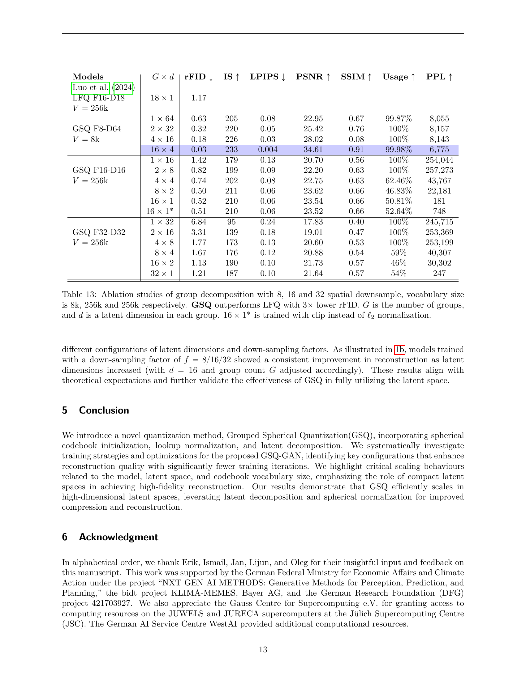
🔼 Table 13 presents a comparison of reconstruction performance using different configurations of the Grouped Spherical Quantization (GSQ) method. The table shows how changing the spatial downsampling factor (8x, 16x, 32x), the codebook vocabulary size (8k, 256k), and the group decomposition (Gx d) affects the reconstruction quality, measured by the rFID (Fréchet Inception Distance). GSQ consistently outperforms LFQ (Lookup-Free Quantizer) achieving a 3x lower rFID. The table also highlights the hyperparameters used in GSQ such as the number of groups (G) and the latent dimension of each group (d). One notable experiment (16 x 1*) used a clip normalization instead of the typical l2 normalization.
read the caption
Table 13: Ablation studies of group decomposition with 8, 16 and 32 spatial downsample, vocabulary size is 8k, 256k and 256k respectively. GSQ outperforms LFQ with 3×3\times3 × lower rFID. G𝐺Gitalic_G is the number of groups, and d𝑑ditalic_d is a latent dimension in each group. 16×1∗16superscript116\times 1^{*}16 × 1 start_POSTSUPERSCRIPT ∗ end_POSTSUPERSCRIPT is trained with clip instead of ℓ2subscriptℓ2\ell_{2}roman_ℓ start_POSTSUBSCRIPT 2 end_POSTSUBSCRIPT normalization.
| rFID ↓ |
|---|
| 256 |
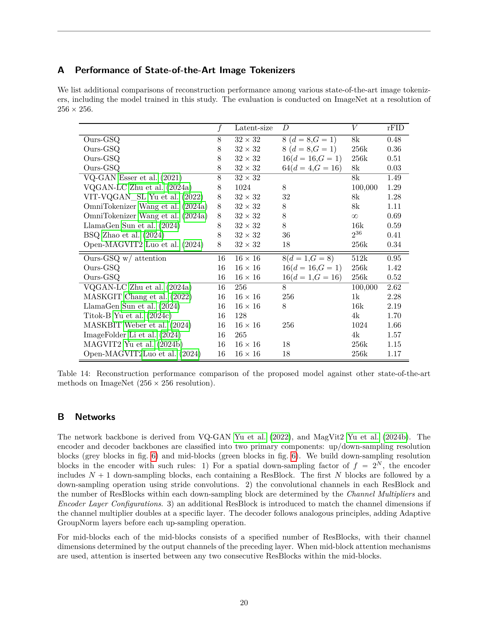
🔼 This table presents a comparison of the reconstruction performance (measured by FID score) of various state-of-the-art image tokenizers on the ImageNet dataset. The models are evaluated using images at a resolution of 256x256 pixels. The table allows for a quantitative comparison of the proposed GSQ model against existing methods, considering factors such as the latent dimension, codebook size and other hyperparameters, providing insights into the model’s relative performance and efficiency.
read the caption
Table 14: Reconstruction performance comparison of the proposed model against other state-of-the-art methods on ImageNet (256×256256256256\times 256256 × 256 resolution).
| Models | G×d | rFID ↓ | IS ↑ | LPIPS ↓ | PSNR ↑ | SSIM ↑ | Usage ↑ | PPL ↑ |
|---|---|---|---|---|---|---|---|---|
| Luo et al. (2024) LFQ F16-D18 V=256k | 18×1 | 1.17 | ||||||
| GSQ F8-D64 V=8k | 1×64 | 0.63 | 205 | 0.08 | 22.95 | 0.67 | 99.87% | 8,055 |
| 2×32 | 0.32 | 220 | 0.05 | 25.42 | 0.76 | 100% | 8,157 | |
| 4×16 | 0.18 | 226 | 0.03 | 28.02 | 0.08 | 100% | 8,143 | |
| 16×4 | 0.03 | 233 | 0.004 | 34.61 | 0.91 | 99.98% | 6,775 | |
| GSQ F16-D16 V=256k | 1×16 | 1.42 | 179 | 0.13 | 20.70 | 0.56 | 100% | 254,044 |
| 2×8 | 0.82 | 199 | 0.09 | 22.20 | 0.63 | 100% | 257,273 | |
| 4×4 | 0.74 | 202 | 0.08 | 22.75 | 0.63 | 62.46% | 43,767 | |
| 8×2 | 0.50 | 211 | 0.06 | 23.62 | 0.66 | 46.83% | 22,181 | |
| 16×1 | 0.52 | 210 | 0.06 | 23.54 | 0.66 | 50.81% | 181 | |
| 16×1* | 0.51 | 210 | 0.06 | 23.52 | 0.66 | 52.64% | 748 | |
| GSQ F32-D32 V=256k | 1×32 | 6.84 | 95 | 0.24 | 17.83 | 0.40 | 100% | 245,715 |
| 2×16 | 3.31 | 139 | 0.18 | 19.01 | 0.47 | 100% | 253,369 | |
| 4×8 | 1.77 | 173 | 0.13 | 20.60 | 0.53 | 100% | 253,199 | |
| 8×4 | 1.67 | 176 | 0.12 | 20.88 | 0.54 | 59% | 40,307 | |
| 16×2 | 1.13 | 190 | 0.10 | 21.73 | 0.57 | 46% | 30,302 | |
| 32×1 | 1.21 | 187 | 0.10 | 21.64 | 0.57 | 54% | 247 |
🔼 This table compares various vector quantization (VQ) methods for image tokenization, showing how they relate to the proposed Grouped Spherical Quantization (GSQ) method. It details the key parameters (latent dimension, codebook size, and the use of techniques like fixed codebooks and ℓ2 normalization) of each method, highlighting how they differ from or are special cases of GSQ. This provides a clear overview of existing methods and clarifies the relationship between GSQ and its predecessors.
read the caption
Table 15: The effective configurations of other tokenizers in GSQ’s view.
| Author | Model | Size |
|---|---|---|
| Luo et al. (2024) | LFQ F16-D18 | V=256k |
🔼 Table 16 presents the hyperparameters used during the training phase of the VAE-F8 model. It details the settings for various aspects of the training process, including training parameters (image resolution, number of training steps, gradient clipping, mixed precision, batch size, and exponential moving average beta), model configuration (downsampling factor, hidden channels, channel multipliers, encoder and decoder layer configurations), quantizer settings (embedding dimension, codebook vocabulary size, and group size), codebook initialization and normalization methods, loss function weights (for reconstruction, perceptual loss using LPIPS, and commitment loss), optimizer settings (type of optimizer, base learning rate, learning rate scheduler, weight decay, betas, and epsilon), providing a comprehensive overview of the training setup.
read the caption
Table 16: VAE-F8 Training Hyperparameters
| f | Latent-size | D | V | rFID |
|---|---|---|---|---|
| Ours-GSQ | 8 | 32x32 | 8 (d=8, G=1) | 8k |
| Ours-GSQ | 8 | 32x32 | 8 (d=8, G=1) | 256k |
| Ours-GSQ | 8 | 32x32 | 16 (d=16, G=1) | 256k |
| Ours-GSQ | 8 | 32x32 | 64 (d=4, G=16) | 8k |
| VQ-GAN [Esser et al. (2021)] | 8 | 32x32 | 8k | |
| VQGAN-LC [Zhu et al. (2024a)] | 8 | 1024 | 8 | 100,000 |
| VIT-VQGAN_SL [Yu et al. (2022)] | 8 | 32x32 | 32 | 8k |
| OmniTokenizer [Wang et al. (2024a)] | 8 | 32x32 | 8 | 8k |
| OmniTokenizer [Wang et al. (2024a)] | 8 | 32x32 | 8 | ∞ |
| LlamaGen [Sun et al. (2024)] | 8 | 32x32 | 8 | 16k |
| BSQ [Zhao et al. (2024)] | 8 | 32x32 | 36 | 2^36 |
| Open-MAGVIT2 [Luo et al. (2024)] | 8 | 32x32 | 18 | 256k |
| Ours-GSQ w/ attention | 16 | 16x16 | 8 (d=1, G=8) | 512k |
| Ours-GSQ | 16 | 16x16 | 16 (d=16, G=1) | 256k |
| Ours-GSQ | 16 | 16x16 | 16 (d=1, G=16) | 256k |
| VQGAN-LC [Zhu et al. (2024a)] | 16 | 256 | 8 | 100,000 |
| MASKGIT [Chang et al. (2022)] | 16 | 16x16 | 256 | 1k |
| LlamaGen [Sun et al. (2024)] | 16 | 16x16 | 8 | 16k |
| Titok-B [Yu et al. (2024c)] | 16 | 128 | 4k | |
| MASKBIT [Weber et al. (2024)] | 16 | 16x16 | 256 | 1024 |
| ImageFolder [Li et al. (2024)] | 16 | 265 | 4k | |
| MAGVIT2 [Yu et al. (2024b)] | 16 | 16x16 | 18 | 256k |
| Open-MAGVIT2 [Luo et al. (2024)] | 16 | 16x16 | 18 | 256k |
🔼 This table presents a qualitative comparison of image reconstruction results obtained using the VAE-F8 model with different configurations: a baseline model, models incorporating Depth2Scale, Adaptive Normalization, and a combination of both Depth2Scale and Adaptive Normalization. The goal is to show the impact of these techniques on image reconstruction quality. Each image shows the original, and the reconstructions.
read the caption
Table 17: Reconstruction results of the VAE-F8 model (in Section 4.1.2) with ablation of Depth2Scale and Adaptive Normalization.
| Finite | Codebook-Sharing | Fixed-Codebook | Effective | ||||||
| VQ | 1 | ✗ | ✗ | ✗ | ✗ | ||||
| VQGAN-ViT | 1 | ✗ | ✗ | ✓ | ✗ | ||||
| LFQ | 1 | 2 | ✗ | ✓ | ✓ | ||||
| FSQ | 1 | ✓ | ✗ | ✓ | ✓ | ||||
| BSQ | 2 | ✗ | ✓ | ✓ | ✓ | ||||
| GSQ | ✗ | ✓ | ✗ |
🔼 Table 18 provides a comprehensive list of hyperparameters used for training the GSQ-GAN model with an 8x spatial downsampling factor. It details both training parameters (e.g., image resolution, number of training steps, batch size) and model configuration settings (e.g., network architecture, latent dimension, codebook size). Furthermore, it specifies the quantization settings, loss weights, optimizer settings, and discriminator configurations used during the GAN training process.
read the caption
Table 18: GAN-F8 Training Hyperparameters
| Parameter | Value |
|---|---|
| Training Parameters | |
| Image Resolution | 128 × 128 |
| Num Train Steps | 100,000 (20 epochs) |
| Gradient Clip | 2 |
| Mixed Precision | BF16 |
| Train Batch Size | 256 |
| Exponential Moving Average Beta | 0.999 |
| Model Configuration | |
| Down-sample-factor (f) | 8 |
| Hidden Channels | 128 |
| Channel Multipliers | [1, 2, 2, 4] |
| Encoder Layer Configs | [2, 2, 2, 2, 2] |
| Decoder Layer Configs | [2, 2, 2, 2, 2] |
| Quantizer Settings | |
| Embed Dimension (D) | 8 |
| Codebook Vocabulary (V) | 8192 |
| Group (G) | 1 |
| Codebook Initialization | ℓ₂(𝒩(0,1)) |
| Look-up Normalization | ℓ₂ |
| Loss weights | |
| Reconstruction Loss | 1.0 |
| Perceptual Loss (LPIPS) | 1.0 |
| Commitment Loss | 0.25 |
| VAE Optimizer | |
| Base Learning Rate | 1 × 10⁻⁴ |
| Learning Rate Scheduler | Fixed |
| Weight Decay | 0.05 |
| Betas | [0.9, 0.95] → [0.9, 0.99] |
| Epsilon | 1 × 10⁻⁸ |
🔼 This table details the architectures of three different discriminators used in the GAN training experiments within the paper: N-Layer, StyleGAN, and DINO. For each discriminator, the table lists the input channels, number of channels, number of layers, and (where applicable) the channel multiplier used in the model architecture. The specific parameters for each discriminator type provide insight into the structural differences used in the training process.
read the caption
Table 19: Discriminator configurations
🔼 This table presents a qualitative comparison of image reconstruction results obtained using different discriminators within the GSQ-GAN-F8 model. The reconstructions of three sample images (a wooden bowl, a rainbow lorikeet, and a library) are displayed for each discriminator configuration. This allows for a visual assessment of the impact of discriminator choice on image generation quality.
read the caption
Table 20: Reconstruction results of the GAN-F8 models (see Section 4.2.1) , trained with different discriminators.
| Parameter | Value |
|---|---|
| Training Parameters | |
| Image Resolution | 128 × 128 |
| Num Train Steps | 80,000 (16 epochs) |
| Gradient Clip | 2 |
| Mixed Precision | BF16 |
| Train Batch Size | 256 |
| Exponential Moving Average Beta | 0.999 |
| Model Configuration | |
| Down-sample-factor (f) | 8 |
| Hidden Channels | 128 |
| Channel Multipliers | [1, 2, 2, 4] |
| Encoder Layer Configs | [2, 2, 2, 2, 2] |
| Decoder Layer Configs | [2, 2, 2, 2, 2] |
| Quantizer Settings | |
| Embed Dimension (D) | 8 |
| Codebook Vocabulary (V) | 8192 |
| Group (G) | 1 |
| Codebook Initialization | ℓ₂(𝒩(0,1)) |
| Look-up Normalization | |
| Discriminator | |
| Name | Dino Discriminator |
| Generator Loss | Non-Saturate |
| Discriminator Loss | Hinge |
| Dino-D Data Augmentation | Cutout+Color+Translation |
| Loss weights | |
| Reconstruction Loss | 1.0 |
| Perceptual Loss (LPIPS) | 1.0 |
| Commitment Loss | 0.25 |
| Adversarial Loss | 0.1 |
| Discriminator Loss | 1.0 |
| VAE Optimizer | |
| Base Learning Rate | 1 × 10⁻⁴ → 2 × 10⁻⁴ |
| Learning Rate Scheduler | Fixed |
| Weight Decay | 0.05 |
| Betas | [0.9, 0.99] |
| Epsilon | 1 × 10⁻⁸ |
| Discriminator Optimizer | |
| Base Learning Rate | 1 × 10⁻⁴ → 2 × 10⁻⁴ |
| Learning Rate Scheduler | Fixed |
| Weight Decay | 0.05 |
| Betas | [0.5, 0.9] → [0.9, 0.99] |
| Epsilon | 1 × 10⁻⁸ |
🔼 Table 21 presents the hyperparameters used during the training phase of the GSQ-GAN model with a downsampling factor of 8. It details settings for various aspects of the training process including image resolution, training steps, gradient clipping, batch size, optimizer parameters, model architecture details (e.g., hidden channels, number of layers in encoder and decoder), quantizer settings (latent dimension, codebook size, group number), loss function weights (reconstruction, perceptual, commitment, adversarial), and discriminator-specific settings. The table offers a comprehensive view of the configuration choices employed to optimize GSQ-GAN’s performance.
read the caption
Table 21: GAN-F8 Training Hyperparameters
| Parameter | Value |
|---|---|
| N-Layer Discriminators (NLD) | |
| Input Channels | 3 |
| Number of Channels | 64 |
| Number of Layers | 3 |
| Style-GAN Discriminators (SGD) | |
| Input Channels | 3 |
| Number of Channels | 128 |
| Channels Multiplier | [2, 4, 4, 4, 4] |
| DINO Discriminators (DD) | |
| Base Model | DinoV2_vits14_reg |
| Channels Multiplier | [2, 4, 4, 4, 4] |
| Features from layer | [2, 5, 8, 11] |
🔼 This table presents a visual comparison of image reconstruction quality across different latent dimensions used in the GSQ-GAN-F8 model. It shows original images alongside reconstructions generated using latent dimensions of 16 (with 1 group), 32 (with 2 groups), and 64 (with 4 groups). The purpose is to demonstrate the impact of latent dimension scaling on the model’s ability to accurately reconstruct images. Figure 1b in the paper provides details about the specific configurations of each model.
read the caption
Table 22: Scaling latent dimension for GSQ-GAN-F8 model. The models are detailed in fig. 1.
🔼 This table presents the results of experiments conducted to analyze how scaling the latent dimension affects the performance of the GSQ-GAN-F16 model. It showcases reconstruction results for different configurations, each varying in latent dimension (D) and number of groups (G). The impact of these changes on the model’s ability to accurately reconstruct images is visually demonstrated through sample images, offering a comparative analysis of the trade-off between latent space complexity and reconstruction quality.
read the caption
Table 23: Scaling latent dimension for GSQ-GAN-F16 model. The models are detailed in fig. 1.
| Parameter | Value |
|---|---|
| Training Parameters | |
| Image Resolution | 256x256 |
| Num Train Steps | 50,000 (20 epochs) |
| Gradient Clip | 2 |
| Mixed Precision | BF16 |
| Train Batch Size | 512 |
| Exponential Moving Average Beta | 0.999 |
| Model Configuration | |
| Down-sample-factor (f) | 8 |
| Hidden Channels | 128 |
| Channel Multipliers | [1, 2, 2, 4] |
| Encoder Layer Configs | [2, 2, 2, 2, 2] |
| Decoder Layer Configs | [2, 2, 2, 2, 2] |
| Discriminator | |
| Name | Dino Discriminator |
| Generator Loss | Non-Saturate |
| Discriminator Loss | Hinge |
| Dino-D Data Augmentation | Cutout+Color+Translation |
| Loss weights | |
| Reconstruction Loss | 1.0 |
| Perceptual Loss (LPIPS) | 1.0 |
| Commitment Loss | 0.25 |
| Adversarial Loss | 0.1 |
| Discriminator Loss | 1.0 |
| VAE and Discriminator Optimizer | |
| Base Learning Rate | 2 × 10⁻⁴ |
| Learning Rate Scheduler | Fixed |
| Weight Decay | 0.05 |
| Betas | [0.9, 0.99] |
| Epsilon | 1 × 10⁻⁸ |
🔼 This table presents results from experiments on scaling the latent dimension of the GSQ-GAN-F32 model. It shows how varying the latent dimension (D) and the number of groups (G), while maintaining a constant overall latent dimensionality (D = d x G), affects the model’s performance. The impact on image reconstruction quality is assessed, and the specific model configurations used in the experiment are referenced in Figure 1 of the paper. The table likely includes metrics such as reconstruction fidelity (rFID), Inception Score (IS), Learned Perceptual Image Patch Similarity (LPIPS), Peak Signal-to-Noise Ratio (PSNR), Structural Similarity Index (SSIM), codebook usage, and perplexity (PPL).
read the caption
Table 24: Scaling latent dimension for GSQ-GAN-F32 model. The models are detailed in fig. 1.
🔼 This table presents an ablation study on scaling the latent dimension in the GSQ-GAN-F8 model, specifically focusing on the impact of varying the number of groups (G) while maintaining a fixed latent dimensionality (D=64) and down-sampling factor (F=8). The study examines how changing the group size affects the model’s reconstruction quality, offering insights into the optimal balance between computational efficiency and representational capacity. Details of the models used in this study are provided in Section 4.3.3 of the paper.
read the caption
Table 25: Scaling latent dimension for GSQ-GAN-F8-D64 model. The models are detailed in Section 4.3.3.
Full paper#
