↗ arXiv ↗ Hugging Face ↗ Papers with Code
TL;DR#
Current methods struggle to unify multimodal understanding and generation due to the different levels of visual detail each task requires. Existing approaches often compromise performance in one area to improve the other, limiting overall effectiveness. A single reconstruction-focused encoder is commonly used for both, but this creates a critical trade-off.
TokenFlow solves this by using a dual-codebook architecture, separating semantic and pixel-level feature learning but linking them through shared indices. This allows direct access to high-level semantic information (for understanding) and fine-grained details (for generation) simultaneously. Extensive experiments demonstrate TokenFlow’s superiority in both understanding and generation, even outperforming models with significantly larger parameter counts. Its high codebook utilization also showcases its efficiency and scalability.
Key Takeaways#
Why does it matter?#
This paper is important because it introduces a novel unified image tokenizer, TokenFlow, that significantly improves performance in both multimodal understanding and generation tasks. It addresses a crucial limitation in existing methods by decoupling semantic and pixel-level feature learning while maintaining alignment, leading to superior results across various benchmarks. This opens new avenues for research in unified multimodal models and efficient visual representation learning. The work’s extensive experimental validation and state-of-the-art results make it highly influential for future research in this area.
Visual Insights#

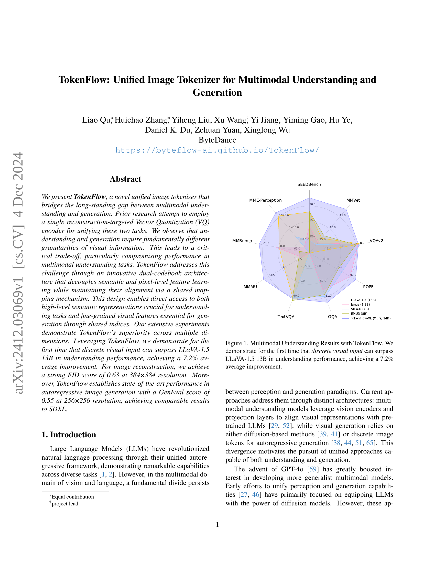
🔼 TokenFlow significantly outperforms LLaVA-1.5 13B on several multimodal understanding benchmarks. The chart visually represents this improvement across different benchmark datasets (MME-Perception, SEEDBench, MM-Vet, VQAv2, TextVQA, GQA). Importantly, this is the first demonstration that a model using discrete visual input (as opposed to continuous representations) achieves better performance than LLaVA-1.5 13B, showcasing a 7.2% average performance increase.
read the caption
Figure 1: Multimodal Understanding Results with TokenFlow. We demonstrate for the first time that discrete visual input can surpass LLaVA-1.5 13B in understanding performance, achieving a 7.2% average improvement.
| # Exp. | Visual Encoder | Type | MME-P ↑ | SEEDB ↑ | TQA ↑ |
|---|---|---|---|---|---|
| Continuous: | |||||
| 1 | CLIP ViT-B/14 [37] | Sem. | 1460.9 | 64.1 | 53.4 |
| Discrete: | |||||
| 2 | VQGAN [13] | Pix. | 756.1 | 38.2 | 46.8 |
| 3 | VQGAN-LC [76] | Pix. | 744.8 | 38.2 | 45.7 |
| 4 | LFQ [66] | Pix. | 889.5 | 41.1 | 46.4 |
| 5 | VQKD [35] | Sem. | 1252.4 | 57.8 | 48.2 |
🔼 This table compares different visual encoders used within the LLaVA-1.5 framework for multimodal understanding tasks. It contrasts continuous encoders (CLIP ViT-B/14) with various discrete encoders (VQGAN, VQGAN-LC, LFQ, VQKD), highlighting the type of visual features they capture (semantic vs. pixel-level). The performance of each encoder is evaluated across three multimodal understanding benchmarks: MME-Perception, SEEDBench, and TextVQA, showcasing the strengths and weaknesses of different approaches in capturing high-level semantic information versus fine-grained visual details.
read the caption
Table 1: Comparison of various visual encoders on multimodal understanding [43, 23, 14] within the LLaVA-1.5 framework. VQKD is distilled from CLIP ViT-B/14. ”Sem.” refers to semantic encoders that learn semantic-level representations, while ”Pix.” indicates pixel-level tokenizers that focus on low-level visual features.
In-depth insights#
Unified Tokenization#
The concept of “Unified Tokenization” in the context of multimodal understanding and generation suggests a paradigm shift towards a single, versatile tokenizer capable of handling both visual and textual data. This contrasts with traditional approaches that employ separate tokenizers optimized for specific modalities, leading to a disconnect between the understanding and generation tasks. A unified tokenizer promises improved efficiency by eliminating the need for multiple models and potentially enhancing the alignment between perception and generation. However, the challenge lies in designing a tokenizer capable of capturing the diverse characteristics of visual data, ranging from high-level semantics for understanding to fine-grained pixel-level details for generation. A successful unified tokenizer would likely require an innovative architecture capable of encoding both semantic and visual information within a shared representation space, enabling seamless integration between modalities. This unified approach has the potential to unlock a more powerful and holistic framework for multimodal AI, but considerable research is needed to address the inherent complexities of such an ambitious task.
Dual-Encoder Design#
A dual-encoder design for image tokenization offers a compelling approach to bridging the gap between multimodal understanding and generation. By employing separate encoders for semantic and pixel-level features, it elegantly addresses the inherent trade-offs between the need for high-level semantic representations in understanding and the requirement for fine-grained visual detail in generation. This decoupling allows each encoder to specialize in its respective task, optimizing feature extraction for each modality without compromise. The key innovation lies in the shared mapping mechanism, aligning the outputs of both encoders via a common index space. This alignment enables the model to access both high-level and low-level visual information seamlessly, providing a unified representation suitable for both understanding and generative tasks. This dual-flow design surpasses single-encoder approaches which often struggle to balance the contrasting demands of these two distinct modalities. The effectiveness of the dual-encoder framework is further enhanced by employing innovative quantization strategies and advanced codebook structures. Ultimately, a dual-encoder architecture offers a powerful and flexible solution, showcasing significant improvements in various multimodal benchmarks.
Multimodal Benchmarks#
Multimodal benchmarks are crucial for evaluating the performance of models that process and integrate information from multiple modalities, such as text and images. A good benchmark should consider several key factors. First, diversity of tasks is essential, encompassing various challenges like visual question answering (VQA), image captioning, visual commonsense reasoning, and others. The benchmark must also include sufficient scale and coverage, with a large number of diverse examples. Data quality and bias mitigation are critical, ensuring the dataset is representative and free from biases that could unfairly skew the results. Further, evaluation metrics should be carefully chosen to align with the specific goals and challenges of each task. Reproducibility and accessibility of the benchmark are also crucial for enabling widespread adoption and comparative analysis of different models. A comprehensive benchmark would enable researchers to track progress in the field, identify areas for improvement, and ultimately drive innovation in the creation of more robust and versatile multimodal models.
Visual Generation#
The research paper section on “Visual Generation” likely details the model’s capacity to produce images from textual descriptions or other prompts. A key aspect would be the architecture employed, possibly involving a transformer network or other deep learning model, trained on a large image-text dataset. The evaluation metrics used to assess image quality are critical, possibly focusing on FID (Fréchet Inception Distance), IS (Inception Score), or other metrics measuring realism, diversity, and adherence to the prompt. The paper would also likely discuss the generation process, explaining how the model translates input into pixel values. This may involve discrete tokenization of images, enabling autoregressive generation, which is particularly efficient. Finally, a comparison with existing state-of-the-art visual generation models would showcase the model’s performance. The paper will likely discuss efficiency gains made via the proposed model, such as fewer sampling steps, lower computational cost and the overall model scalability. Qualitative examples of generated images, illustrating the model’s capabilities in various styles and scenarios are also expected.
Future of TokenFlow#
The future of TokenFlow looks promising, building upon its strengths in unifying multimodal understanding and generation. Further research could explore expanding the dual-codebook architecture to incorporate additional modalities, such as audio or depth information, creating even richer representations for more complex tasks. Improving the scalability and efficiency of the model, particularly during inference, is another key area. This could involve exploring more efficient quantization techniques or architectural optimizations. Addressing the performance gap between TokenFlow and its continuous counterparts remains a crucial goal, potentially achievable through advanced training strategies or a refined codebook design. The potential for TokenFlow extends to broader applications in areas like interactive image editing and creative content generation, where its ability to seamlessly integrate semantic and pixel-level understanding could be transformative. Ultimately, the open-source nature of TokenFlow encourages community contributions and further development, accelerating its evolution into a truly versatile multimodal engine.
More visual insights#
More on figures

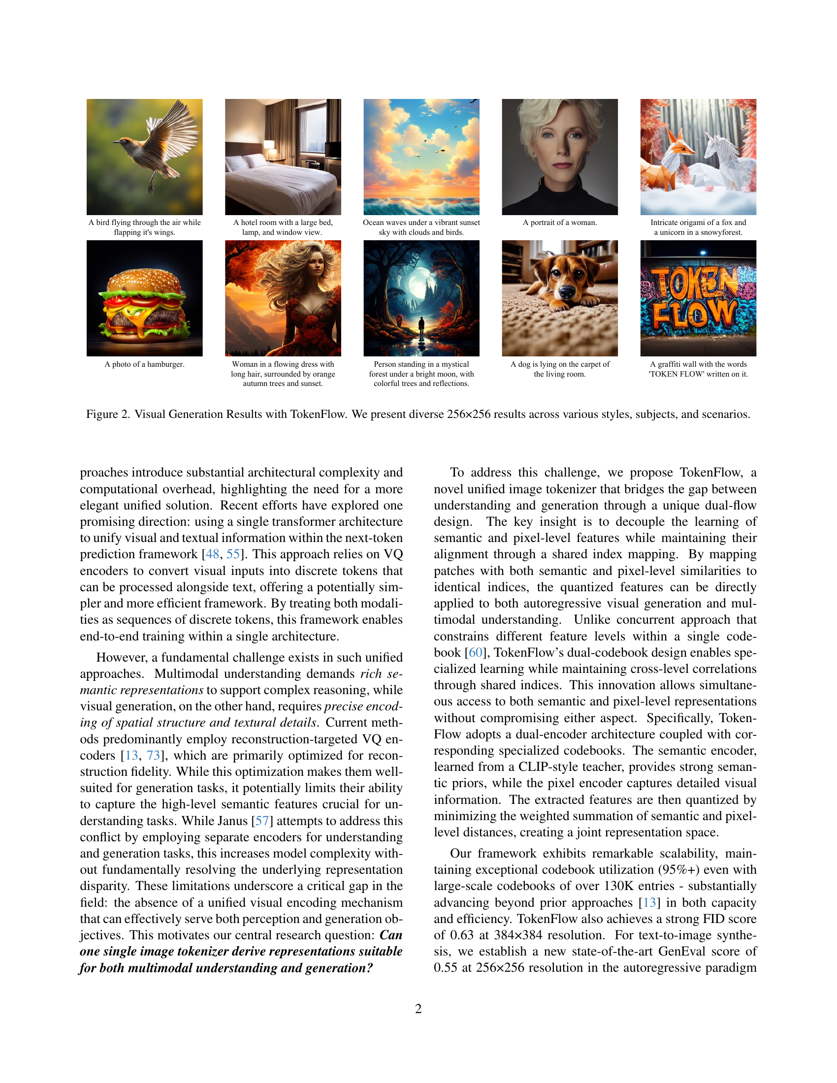
🔼 This figure showcases the diverse image generation capabilities of the TokenFlow model. It displays a variety of 256x256 pixel images, demonstrating the model’s ability to generate images in different artistic styles, depicting a wide range of subjects and scenes. The visual variety highlights the model’s flexibility and robustness across diverse image generation tasks.
read the caption
Figure 2: Visual Generation Results with TokenFlow. We present diverse 256×256 results across various styles, subjects, and scenarios.

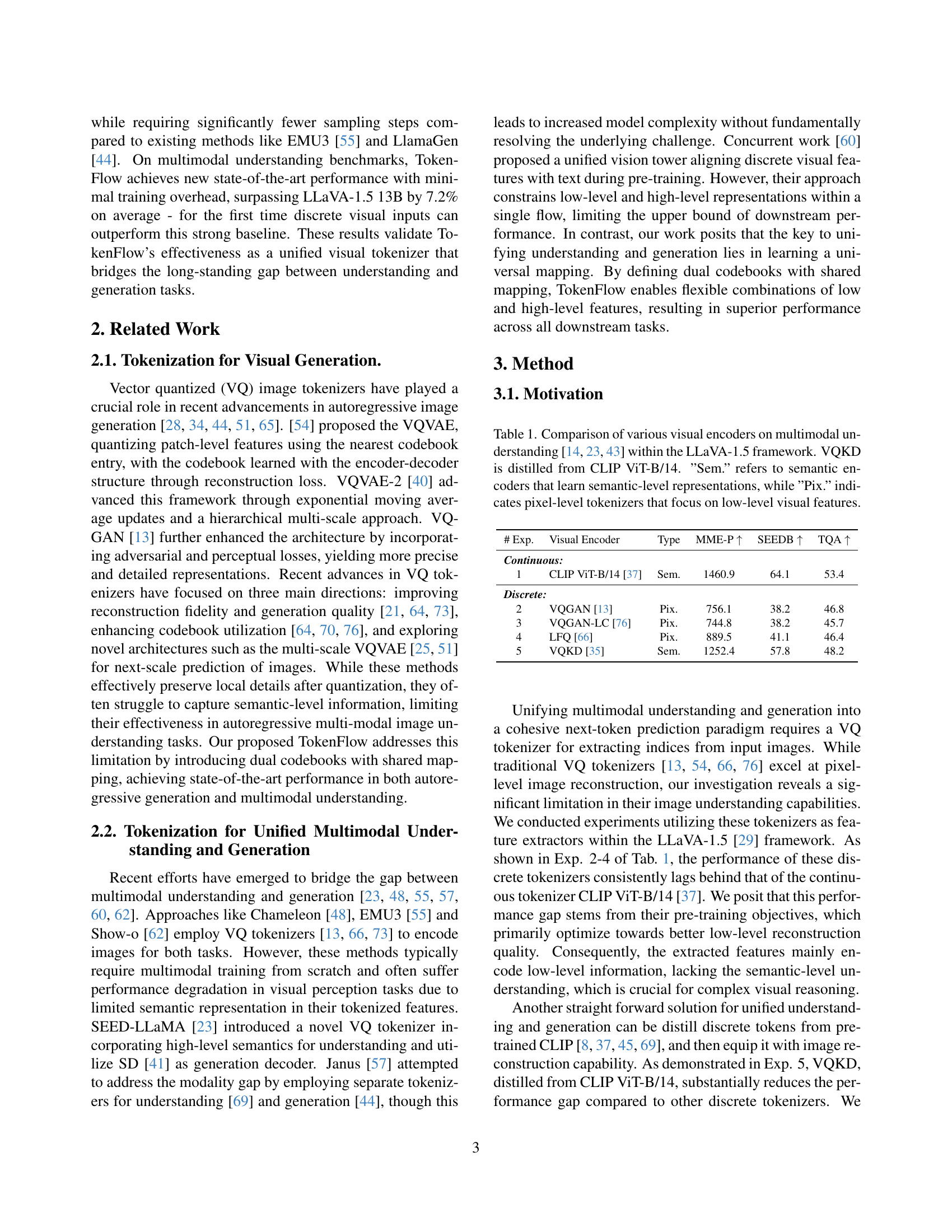
🔼 TokenFlow uses a dual-encoder architecture with two codebooks (semantic and pixel) and a shared mapping mechanism. The semantic encoder focuses on high-level semantic features, while the pixel encoder captures fine-grained visual details. Both encoders’ outputs are quantized using a weighted sum of their distances to the respective codebooks, resulting in a unified index and features that represent both semantic and pixel information. These features are then independently decoded for semantic alignment and image reconstruction before being concatenated into a unified representation used by downstream tasks (multimodal understanding and generation).
read the caption
Figure 3: Overview of TokenFlow. We incorporate dual encoders and codebooks with a shared mapping, enabling the joint optimization of high-level semantics and low-level pixel details. For a given input image, distances dsemsubscript𝑑semd_{\text{sem}}italic_d start_POSTSUBSCRIPT sem end_POSTSUBSCRIPT and dpixsubscript𝑑pixd_{\text{pix}}italic_d start_POSTSUBSCRIPT pix end_POSTSUBSCRIPT are calculated from the pixel-level and semantic-level codebooks, respectively, with the final codebook index and features determined by minimizing the weighted sum dsem+wdis⋅dpixsubscript𝑑sem⋅subscript𝑤dissubscript𝑑pixd_{\text{sem}}+w_{\text{dis}}\cdot d_{\text{pix}}italic_d start_POSTSUBSCRIPT sem end_POSTSUBSCRIPT + italic_w start_POSTSUBSCRIPT dis end_POSTSUBSCRIPT ⋅ italic_d start_POSTSUBSCRIPT pix end_POSTSUBSCRIPT. The resulting quantized features are independently decoded for both semantic alignment and image reconstruction training, and then concatenated to provide a unified representation for downstream tasks in understanding and generation.

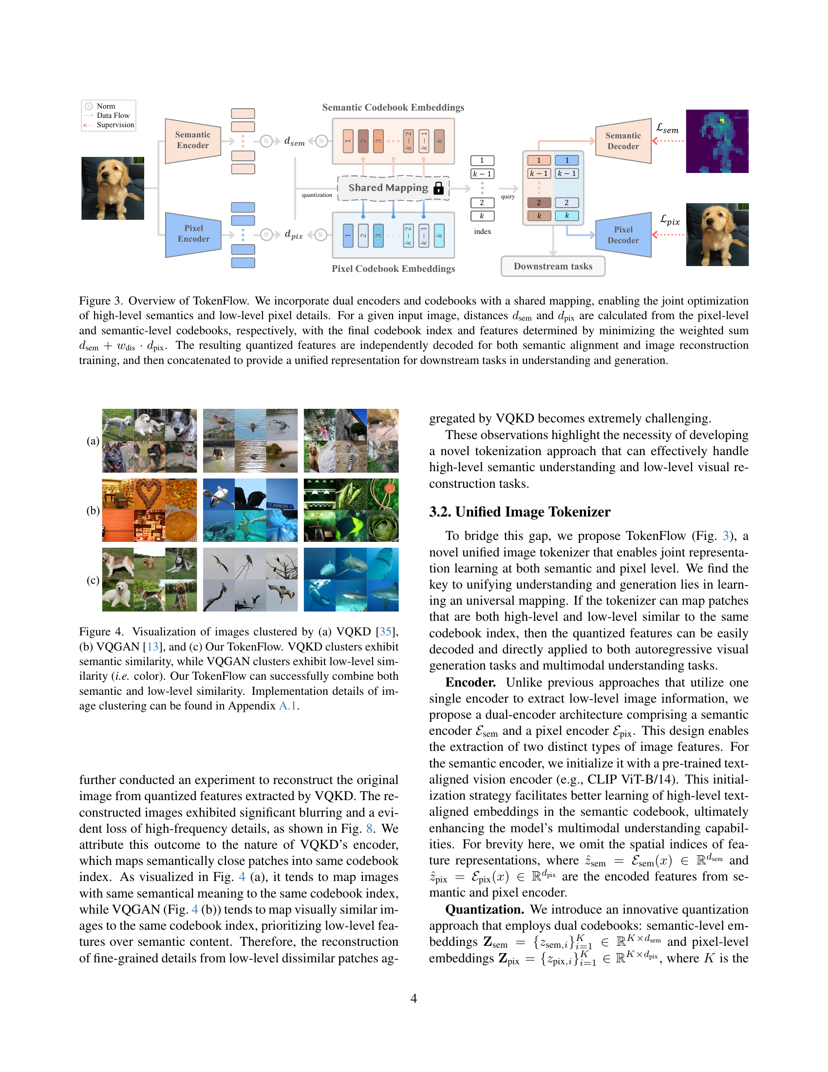
🔼 This figure compares the clustering results of three different image tokenizers: VQKD, VQGAN, and TokenFlow. VQKD, designed for semantic understanding, groups images based on their semantic similarity, even if they have different visual appearances. VQGAN, focused on image generation, groups images based on low-level visual features like color and texture, even if semantically different. TokenFlow, the proposed method, successfully combines both semantic and low-level visual features in its clustering, demonstrating its ability to capture a richer representation of image content. This is crucial for both image understanding and generation tasks.
read the caption
Figure 4: Visualization of images clustered by (a) VQKD [35], (b) VQGAN [13], and (c) Our TokenFlow. VQKD clusters exhibit semantic similarity, while VQGAN clusters exhibit low-level similarity (i.e. color). Our TokenFlow can successfully combine both semantic and low-level similarity. Implementation details of image clustering can be found in Sec. A.1.

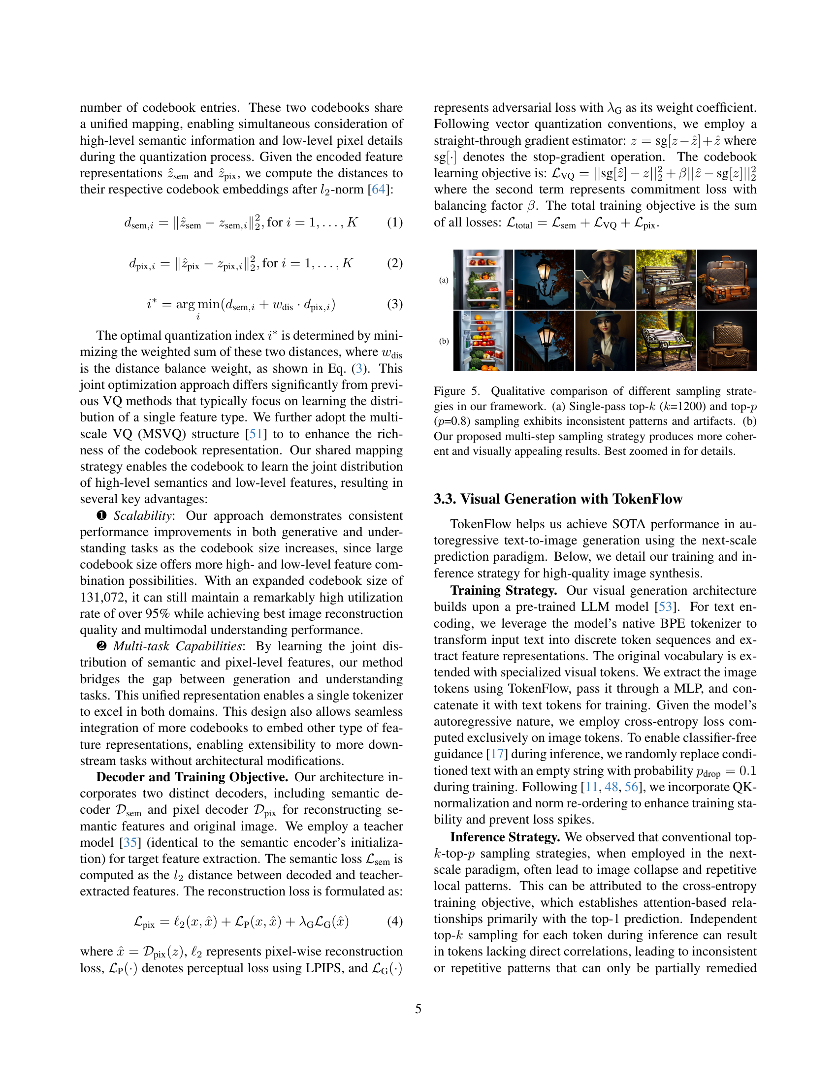
🔼 This figure compares two image sampling strategies. The first uses a single-pass approach with top-k=1200 and top-p=0.8, resulting in images with inconsistent patterns and artifacts. The second, proposed by the authors, is a multi-step strategy that yields more coherent and visually pleasing results, as shown in the images. Zooming in on the images reveals more detail.
read the caption
Figure 5: Qualitative comparison of different sampling strategies in our framework. (a) Single-pass top-k𝑘kitalic_k (k𝑘kitalic_k=1200) and top-p𝑝pitalic_p (p𝑝pitalic_p=0.8) sampling exhibits inconsistent patterns and artifacts. (b) Our proposed multi-step sampling strategy produces more coherent and visually appealing results. Best zoomed in for details.

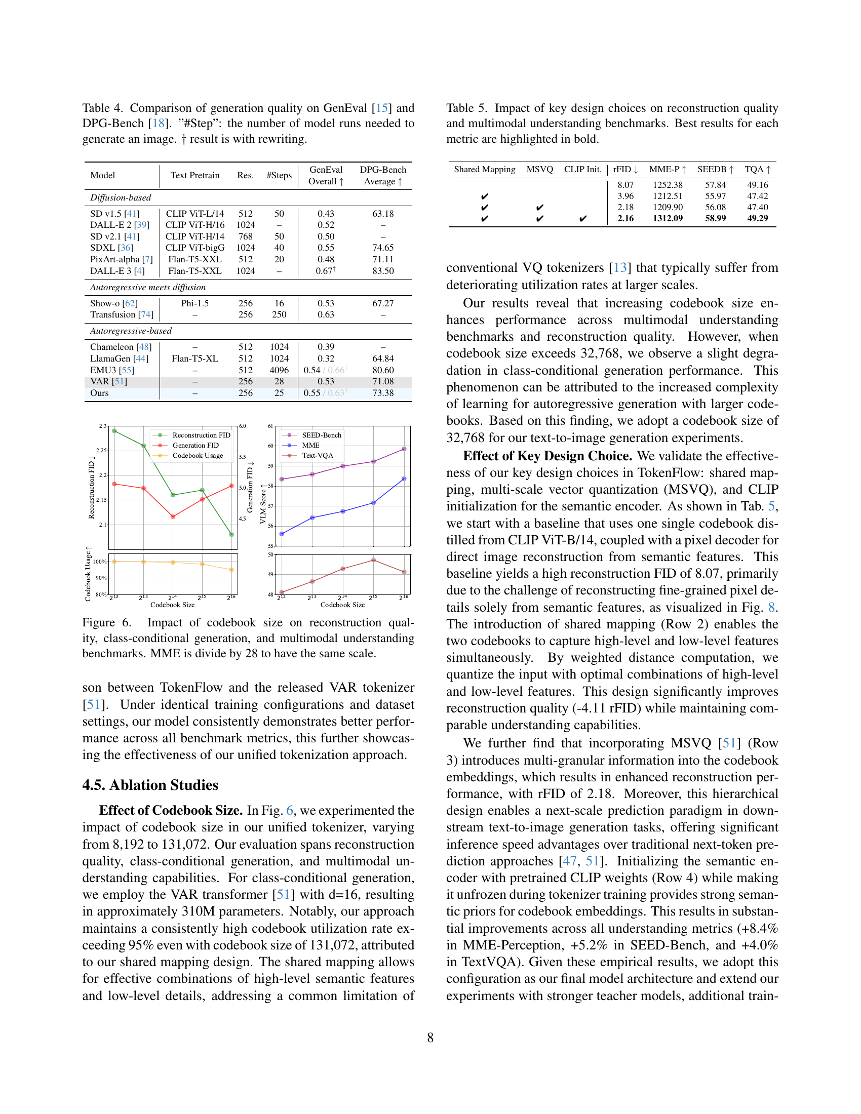
🔼 This figure analyzes how varying the codebook size in the TokenFlow model affects its performance across three key areas: image reconstruction quality (measured by FID), class-conditional image generation (measured by FID), and multimodal understanding benchmarks (measured by MME, SEED-Bench, and TextVQA). The results show the trade-off between these aspects as the codebook size increases. The MME score is divided by 28 for consistent scaling.
read the caption
Figure 6: Impact of codebook size on reconstruction quality, class-conditional generation, and multimodal understanding benchmarks. MME is divide by 28 to have the same scale.

🔼 This figure compares the distribution of cluster sizes for three different image tokenization methods: VQKD, VQGAN, and TokenFlow. Using a fixed codebook size of 8,192, the methods were tested on 50,000 images from the ImageNet-1k validation set. The plot shows that TokenFlow’s distribution of cluster sizes is significantly more uniform than those of VQKD and VQGAN. This smoother distribution is attributed to TokenFlow’s novel shared mapping design, which learns joint distributions of semantic and pixel-level features. This dual-feature learning approach results in consistently high codebook utilization (over 95%), even with significantly larger codebooks (over 131,000 entries). This high utilization rate highlights the efficiency of TokenFlow’s architecture and its effectiveness in capturing both high-level semantic information and fine-grained visual detail.
read the caption
Figure 7: Comparison of cluster size distributions between VQKD [35], VQGAN [13], and TokenFlow (ours), with a fixed codebook size of 8,192. Analysis performed on 50,000 images from the ImageNet-1k validation set. TokenFlow exhibits significantly smoother distribution compared to others, attributed to our shared mapping design that learns joint distributions of semantic and pixel-level features. This joint learning approach helps maintain high codebook utilization (95%+) even with large-scale codebooks containing over 131K entries.

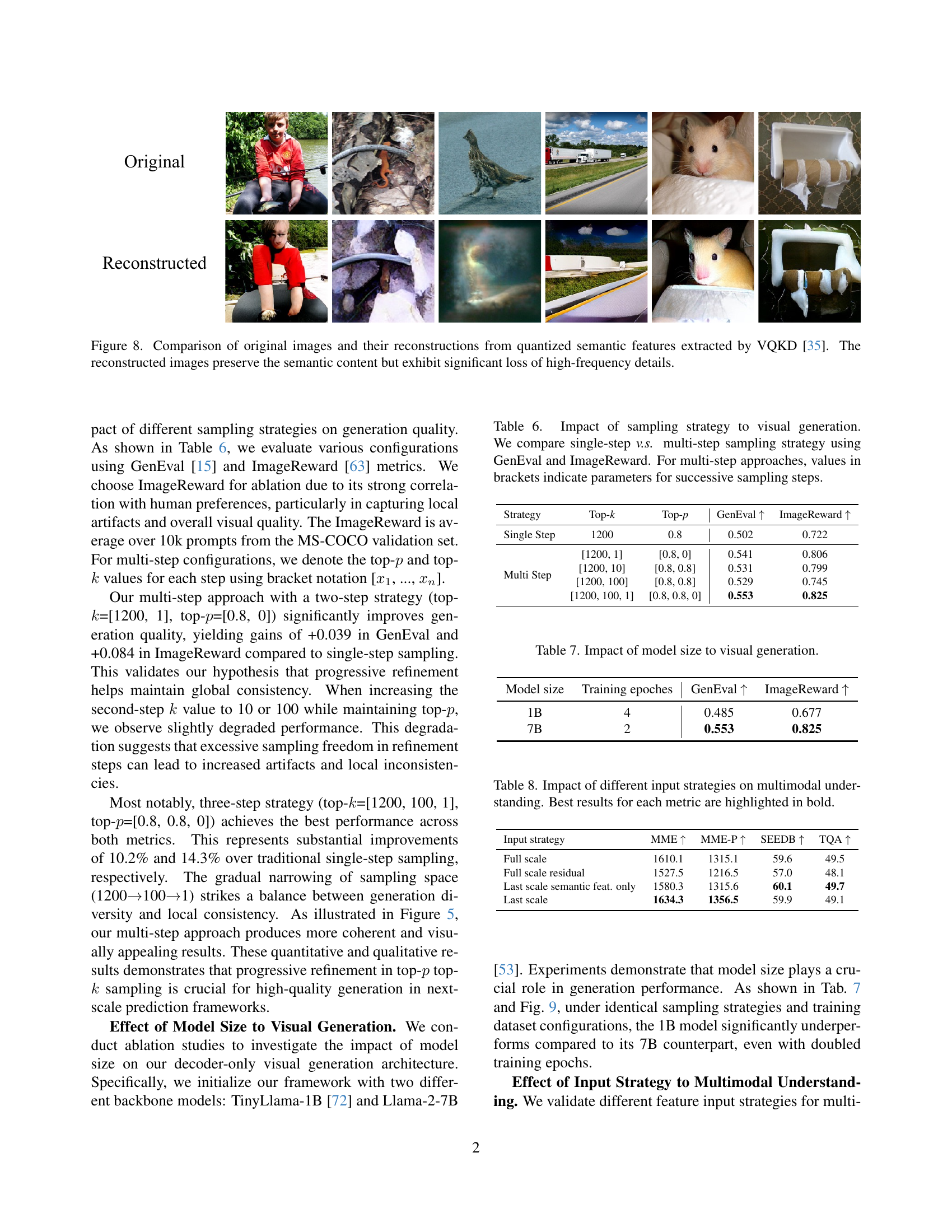
🔼 This figure displays a comparison between original images from the ImageNet-1k dataset and their reconstructions from quantized semantic features using VQKD [35]. The reconstruction process, while preserving the overall semantic meaning of the images (e.g., the subject matter), results in a significant loss of fine details and high-frequency information. This demonstrates a key limitation of solely relying on semantic features for image reconstruction; such an approach struggles to capture the sharpness and intricate texture present in the original images.
read the caption
Figure 8: Comparison of original images and their reconstructions from quantized semantic features extracted by VQKD [35]. The reconstructed images preserve the semantic content but exhibit significant loss of high-frequency details.

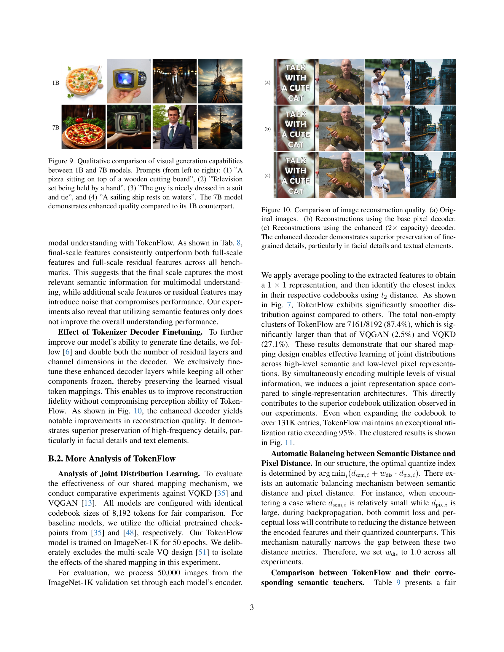
🔼 This figure showcases a qualitative comparison of image generation results from two different sized models: a 1B parameter model and a 7B parameter model. Four different prompts were used to generate the images. The prompts are: 1) ‘A pizza sitting on top of a wooden cutting board’, 2) ‘Television set being held by a hand’, 3) ‘The guy is nicely dressed in a suit and tie’, and 4) ‘A sailing ship rests on waters’. The results clearly demonstrate that the larger, 7B parameter model produces images with significantly higher visual fidelity and detail compared to the smaller model.
read the caption
Figure 9: Qualitative comparison of visual generation capabilities between 1B and 7B models. Prompts (from left to right): (1) ”A pizza sitting on top of a wooden cutting board”, (2) ”Television set being held by a hand”, (3) ”The guy is nicely dressed in a suit and tie”, and (4) ”A sailing ship rests on waters”. The 7B model demonstrates enhanced quality compared to its 1B counterpart.

🔼 This figure compares the image reconstruction quality using different decoders. The original images are shown in (a). (b) shows reconstructions using the base pixel decoder, which has limitations in preserving fine details. (c) shows the improvement achieved by using an enhanced decoder with double the capacity, resulting in significantly better reconstruction of fine details such as facial features and text.
read the caption
Figure 10: Comparison of image reconstruction quality. (a) Original images. (b) Reconstructions using the base pixel decoder. (c) Reconstructions using the enhanced (2×2\times2 × capacity) decoder. The enhanced decoder demonstrates superior preservation of fine-grained details, particularly in facial details and textual elements.

🔼 This figure compares the clustering results of three different image tokenizers: VQKD, VQGAN, and TokenFlow. VQKD, focused on semantic meaning, groups images with similar concepts together regardless of visual details. VQGAN, prioritizing low-level visual features, clusters images based on similarities in color and texture. TokenFlow, in contrast, successfully combines both semantic and low-level features in its clustering. This allows it to group images that share both conceptual meaning and visual characteristics. The example given highlights this advantage by showing how birds with different backgrounds are clustered together by TokenFlow, reflecting both their semantic (birds) and visual (shared feature) similarities, whereas the other two methods would separate them.
read the caption
Figure 11: Qualitative comparison of images clustered by VQKD [35], VQGAN [13] and our TokenFlow. VQKD clusters exhibit semantic similarity, while VQGAN clusters exhibit low-level similarity (i.e. color and texture). Our TokenFlow can successfully combine both semantic and low-level similarity (e.g. birds with different background can be mapped into two different index).

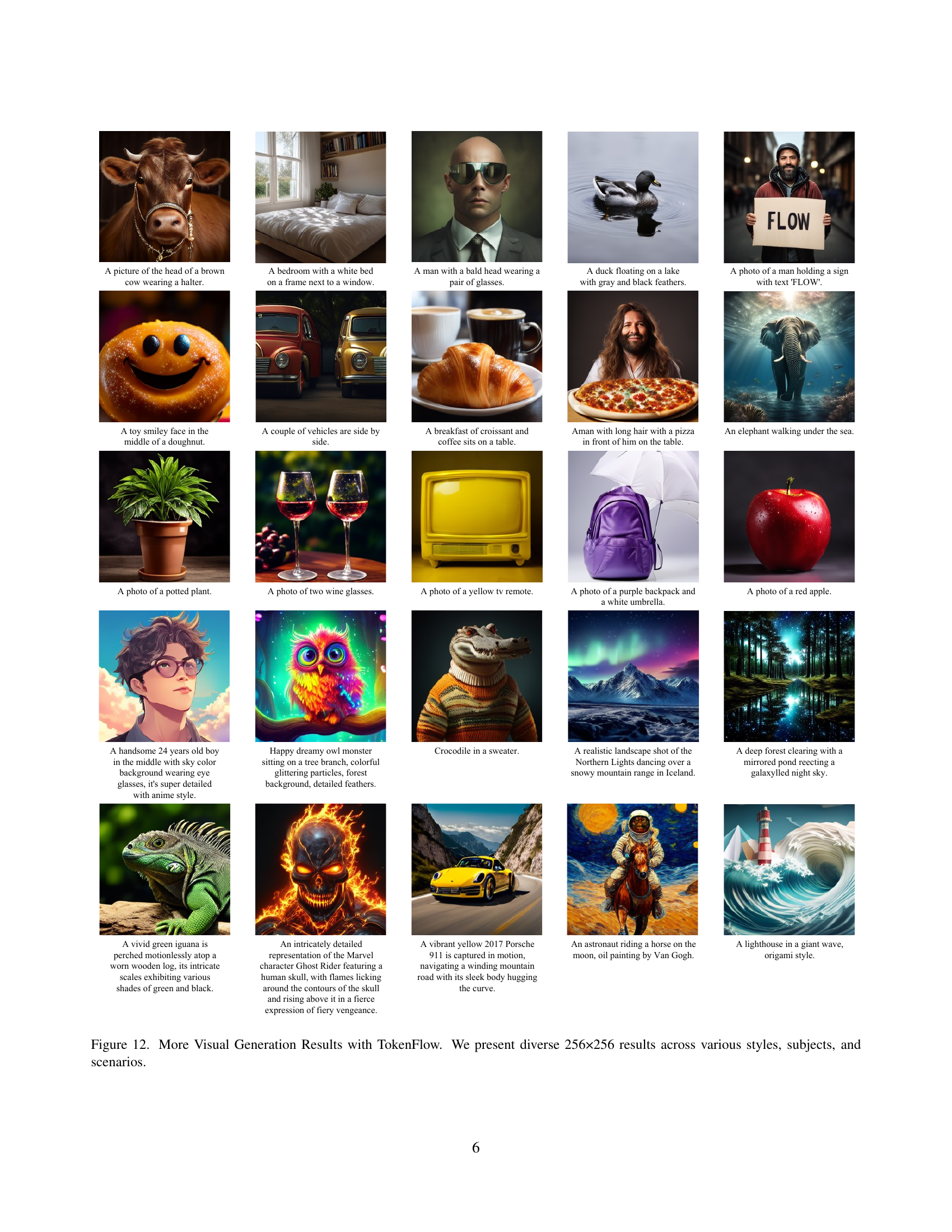
🔼 This figure showcases the diverse image generation capabilities of the TokenFlow model. It presents a variety of 256x256 pixel images, demonstrating the model’s ability to generate images across a wide range of styles, subjects, and scenarios. The examples highlight the model’s versatility in generating photorealistic images, artistic renderings, and imaginative compositions.
read the caption
Figure 12: More Visual Generation Results with TokenFlow. We present diverse 256×256 results across various styles, subjects, and scenarios.
More on tables
| Model | Res. | ratio | #Lvls. | rFID ↓ | PSNR ↑ | SSIM ↑ |
|---|---|---|---|---|---|---|
| VQ-GAN [13] | 256 | 16 | 1 | 4.98 | 20.00 | 0.629 |
| LlamaGen [44] | 256 | 16 | 1 | 2.19 | 20.79 | 0.675 |
| RQ-VAE [21] | 256 | 32 | 4 | 3.20 | – | – |
| RQ-VAE [21] | 256 | 16 | 4 | 1.30 | – | – |
| VAR [51] | 256 | 16 | 10 | 1.00 | 22.63 | 0.755 |
| VILA-U [60] | 256 | 16 | 4 | 1.80 | – | – |
| Ours | 256 | 16 | 9 | 1.37 | 21.41 | 0.687 |
| LlamaGen [60] | 384 | 14.2 | 1 | 0.94 | 21.94 | 0.726 |
| VILA-U [60] | 384 | 14.2 | 16 | 1.25 | – | – |
| VAR [51] | 384 | 16 | 13 | 2.09 | 22.73 | 0.774 |
| Ours | 384 | 14.2 | 15 | 0.63 | 22.77 | 0.731 |
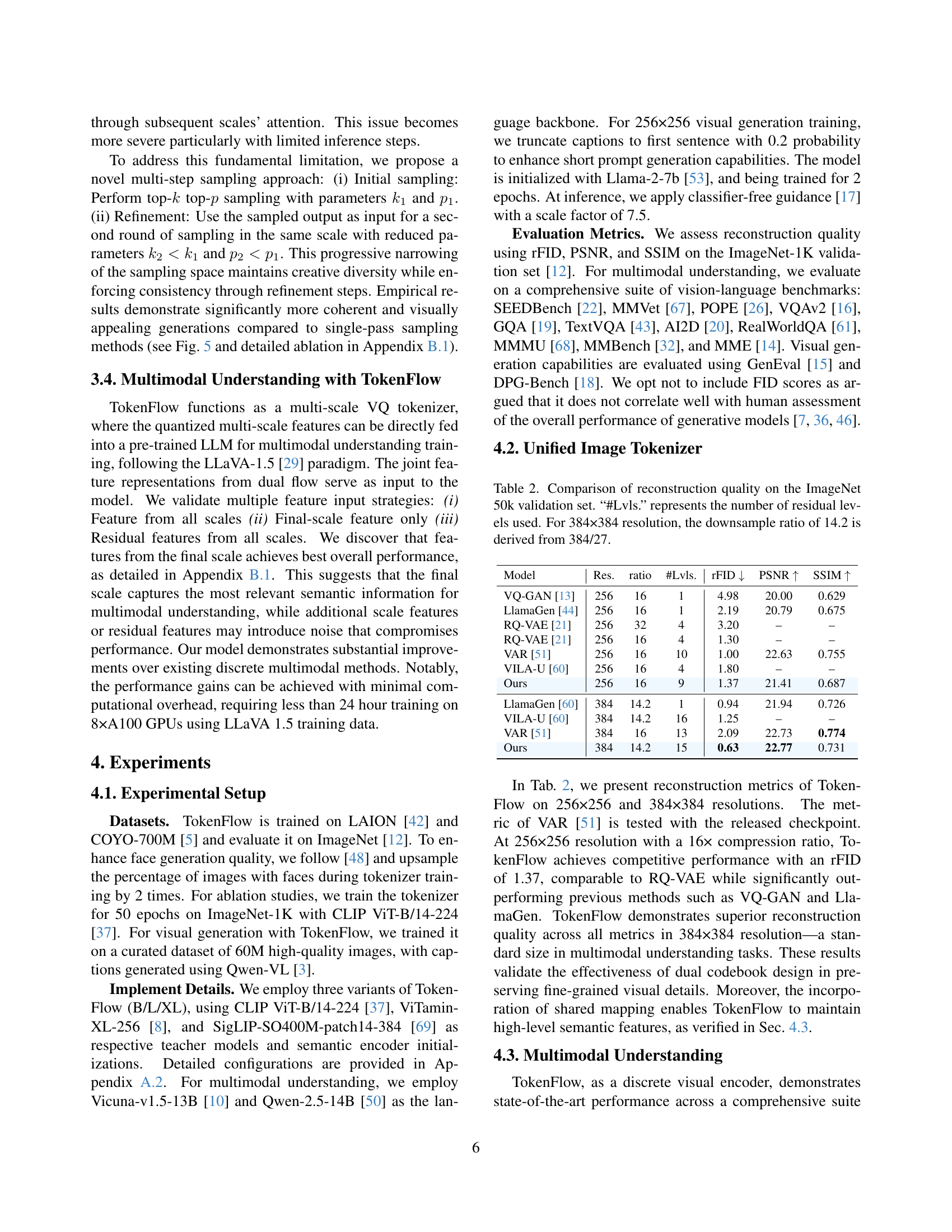
🔼 This table compares the reconstruction quality of different models on the ImageNet 50k validation set. The quality is assessed using three metrics: rFID (lower is better, indicating better fidelity to the original images), PSNR (higher is better, representing the ratio of the maximum possible power of a signal to the power of the noise), and SSIM (higher is better, measuring structural similarity). The table also indicates the resolution of the images (256x256 or 384x384 pixels), the downsampling ratio used (16 or 14.2, representing how much the original image was reduced in size before processing), and the number of residual levels (’#Lvls.’) used in the model’s architecture (a higher number indicates more complex processing). The purpose is to show how TokenFlow compares to existing image generation models in terms of reconstruction accuracy.
read the caption
Table 2: Comparison of reconstruction quality on the ImageNet 50k validation set. “#Lvls.” represents the number of residual levels used. For 384×384 resolution, the downsample ratio of 14.2 is derived from 384/27.
| Method | # Params | Res. | SEEDB | MMV | POPE | VQAv2 | GQA | TQA | AI2D | RWQA | MMMU | MMB | MME | MME-P | Avg. |
|---|---|---|---|---|---|---|---|---|---|---|---|---|---|---|---|
| Continuous Visual Input | |||||||||||||||
| InstructBLIP [30] | Vicuna-13B | 224 | 58.8 | 25.6 | 78.9 | – | 49.5 | 50.7 | – | – | – | 36.0 | – | 1212.8 | – |
| MiniGPT-4 [75] | Vicuna-13B | 224 | – | – | – | – | – | – | – | – | – | – | 1158.7 | 866.6 | – |
| BLIP-2 [24] | Vicuna-13B | 224 | 46.4 | 22.4 | – | – | – | 42.5 | – | – | 26.6 | – | – | 1293.8 | – |
| ShareGPT4V [9] | Vicuna-7B | 336 | 69.7 | 37.6 | – | 80.6 | 63.3 | 60.4 | 58.0 | 54.9 | 37.2 | 68.8 | 1943.8 | 1567.4 | – |
| NExT-GPT [58] | Vicuna-7B | 224 | 57.5 | – | – | 66.0 | – | – | – | – | – | 58.0 | – | – | – |
| Qwen-VL-Chat [3] | Qwen-7B | 448 | 57.7 | – | – | 78.2 | 57.5 | – | – | – | – | – | 1848.3 | 1487.5 | – |
| Janus [57] | DeepSeek-LLM-1.3B | 384 | 63.7 | 34.3 | 87.0 | 77.3 | 59.1 | – | – | – | 30.5 | 69.4 | – | 1338.0 | – |
| LLaVA-1.5 [29] | Vicuna-13B | 336 | 68.1 | 36.1 | 85.9 | 80.0 | 63.3 | 61.3 | 61.1 | 55.3 | 36.4 | 67.7 | 1826.7 | 1531.3 | 62.9 |
| Discrete Visual Input | |||||||||||||||
| Gemini-Nano-1 [49] | 1.8B from scratch | – | – | – | – | 62.7 | – | – | – | – | 26.3 | – | – | – | – |
| Chameleon [48] | 34B from scratch | 256 | – | – | – | 69.6 | – | – | – | – | – | – | – | – | – |
| LWM [31] | LLaMA-2-7B | 256 | – | 9.6 | 75.2 | 55.8 | 44.8 | 18.8 | – | – | – | – | – | – | – |
| SEED-LLaMA [23] | LLaMA-2-13B | 224 | 53.7 | – | – | 63.4 | – | – | – | – | – | – | – | – | – |
| Show-o [62] | Phi-1.5-1.3B | 256 | – | – | 80.0 | 69.4 | 58.0 | – | – | – | 26.7 | – | – | 1097.2 | – |
| VILA-U [60] | LLaMA-2-7B | 256 | 56.3 | 27.7 | 83.9 | 75.3 | 58.3 | 48.3 | – | – | – | – | – | 1336.2 | – |
| VILA-U [60] | LLaMA-2-7B | 384 | 59.0 | 33.5 | 85.8 | 79.4 | 60.8 | 60.8 | – | – | – | – | – | 1401.8 | – |
| EMU3 [55] | 8B from scratch | 512 | 68.2 | 37.2 | 85.2 | 75.1 | 60.3 | 64.7 | 70.0 | 57.4 | 31.6 | 58.5 | 1509.9* | 1243.8* | 60.9 |
| TokenFlow-B | Vicuna-13B | 224 | 60.4 | 22.4 | 84.0 | 70.2 | 59.3 | 49.8 | 54.2 | 49.4 | 34.2 | 55.3 | 1660.4 | 1353.6 | 55.2 |
| TokenFlow-L | Vicuna-13B | 256 | 62.6 | 27.7 | 85.0 | 73.9 | 60.3 | 54.1 | 56.6 | 49.2 | 34.4 | 60.3 | 1622.9 | 1365.4 | 57.5 |
| TokenFlow-XL | Vicuna-13B | 384 | 68.7 | 40.7 | 86.8 | 77.9 | 62.7 | 61.5 | 66.7 | 53.7 | 38.7 | 68.9 | 1840.9 | 1545.9 | 64.0 |
| TokenFlow-XL | Qwen-2.5-14B | 384 | 72.6 | 48.2 | 87.8 | 77.6 | 62.5 | 62.3 | 75.8 | 56.6 | 43.2 | 76.8 | 1922.2 | 1551.1 | 67.4 |
🔼 Table 3 presents a comprehensive evaluation of various models’ performance on a range of multimodal understanding benchmarks. These benchmarks assess different aspects of vision-language capabilities, including image-text matching, visual question answering, and commonsense reasoning. The table categorizes models into two groups: those using continuous visual inputs (like those directly from a vision transformer) and those using discrete visual inputs (like those from a vector quantized image tokenizer). The best-performing models within the discrete visual input category are highlighted in bold. Some results marked with an asterisk (*) were not originally reported in the cited papers but were obtained using a separate evaluation tool (lmms-eval [71]) and a publicly released checkpoint. Finally, to ensure consistent scaling across different benchmarks, the MME-Perception score was divided by 20 when calculating the average score.
read the caption
Table 3: Evaluation on multimodal understanding benchmarks. We collect evaluations including: SEEDB: SEED Bench-Img [22]; MMV: MM-Vet [67]; POPE [26]; VQAv2 [16]; GQA [19]; TQA: TextVQA [43]; AI2D [20]; RWQA: RealWorldQA [61]; MMMU [68]; MMB: MMBench [32]; MME [14] and MME-P: MME-Perception. We include approaches with continuous visual inputs (top) versus discrete visual inputs (bottom). The best results among approaches with discrete visual input are highlighted in bold. * results are not reported in original paper and tested with lmms-eval [71] using the released checkpoint. When calculating average, we use MME-P and divide it by 20 to have the same scale with other benchmarks.
| Model | Text Pretrain | Res. | #Steps | GenEval ↑ | DPG-Bench ↑ |
|---|---|---|---|---|---|
| Diffusion-based | |||||
| SD v1.5 [41] | CLIP ViT-L/14 | 512 | 50 | 0.43 | 63.18 |
| DALL-E 2 [39] | CLIP ViT-H/16 | 1024 | – | 0.52 | – |
| SD v2.1 [41] | CLIP ViT-H/14 | 768 | 50 | 0.50 | – |
| SDXL [36] | CLIP ViT-bigG | 1024 | 40 | 0.55 | 74.65 |
| PixArt-alpha [7] | Flan-T5-XXL | 512 | 20 | 0.48 | 71.11 |
| DALL-E 3 [4] | Flan-T5-XXL | 1024 | – | 0.67† | 83.50 |
| Autoregressive meets diffusion | |||||
| Show-o [62] | Phi-1.5 | 256 | 16 | 0.53 | 67.27 |
| Transfusion [74] | – | 256 | 250 | 0.63 | – |
| Autoregressive-based | |||||
| Chameleon [48] | – | 512 | 1024 | 0.39 | – |
| LlamaGen [44] | Flan-T5-XL | 512 | 1024 | 0.32 | 64.84 |
| EMU3 [55] | – | 512 | 4096 | 0.54 / 0.66† | 80.60 |
| VAR [51] | – | 256 | 28 | 0.53 | 71.08 |
| Ours | – | 256 | 25 | 0.55 / 0.63† | 73.38 |
🔼 This table compares the image generation quality of different models using two metrics: GenEval and DPG-Bench. GenEval assesses the overall quality of generated images, while DPG-Bench evaluates various aspects like object, attribute, and color accuracy. The ‘#Step’ column indicates how many times the model needs to run to generate a single image. A ‘+’ symbol next to a result suggests that additional prompt rewriting techniques were used to enhance generation quality.
read the caption
Table 4: Comparison of generation quality on GenEval [15] and DPG-Bench [18]. ”#Step”: the number of model runs needed to generate an image. ††\dagger† result is with rewriting.
| Shared Mapping | MSVQ | CLIP Init. | rFID ↓ | MME-P ↑ | SEEDB ↑ | TQA ↑ |
|---|---|---|---|---|---|---|
| 8.07 | 1252.38 | 57.84 | 49.16 | |||
| ✓ | 3.96 | 1212.51 | 55.97 | 47.42 | ||
| ✓ | ✓ | 2.18 | 1209.90 | 56.08 | 47.40 | |
| ✓ | ✓ | ✓ | 2.16 | 1312.09 | 58.99 | 49.29 |
🔼 This table presents an ablation study analyzing the impact of key design choices in TokenFlow on both image reconstruction quality and multimodal understanding performance. It compares the results using different configurations: with and without shared mapping, with and without multi-scale vector quantization (MSVQ), and with and without initializing the semantic encoder using CLIP. The metrics used to evaluate reconstruction quality include FID (Fréchet Inception Distance), while the multimodal understanding benchmarks are MME-P, SEEDB, and TQA. The best results for each metric across all configurations are highlighted in bold.
read the caption
Table 5: Impact of key design choices on reconstruction quality and multimodal understanding benchmarks. Best results for each metric are highlighted in bold.
| Strategy | Top-k | Top-p | GenEval ↑ | ImageReward ↑ |
|---|---|---|---|---|
| Single Step | 1200 | 0.8 | 0.502 | 0.722 |
| Multi Step | [1200, 1] | [0.8, 0] | 0.541 | 0.806 |
| [1200, 10] | [0.8, 0.8] | 0.531 | 0.799 | |
| [1200, 100] | [0.8, 0.8] | 0.529 | 0.745 | |
| [1200, 100, 1] | [0.8, 0.8, 0] | 0.553 | 0.825 |
🔼 This table investigates the effect of different sampling strategies on the quality of visual generation. It compares single-step sampling methods against multi-step approaches. The evaluation metrics used are GenEval and ImageReward. For multi-step sampling, the table details the top-k and top-p parameters used in each successive sampling step, allowing for a detailed analysis of how these parameters influence the final generated image.
read the caption
Table 6: Impact of sampling strategy to visual generation. We compare single-step v.s. multi-step sampling strategy using GenEval and ImageReward. For multi-step approaches, values in brackets indicate parameters for successive sampling steps.
| Model size | Training epoches | GenEval ↑ | ImageReward ↑ |
|---|---|---|---|
| 1B | 4 | 0.485 | 0.677 |
| 7B | 2 | 0.553 | 0.825 |
🔼 This table presents the results of an ablation study on the impact of model size on visual generation performance. It shows how different model sizes (1B and 7B parameters) affect the GenEval and ImageReward metrics, key measures of visual generation quality. The table also indicates the number of training epochs used for each model size.
read the caption
Table 7: Impact of model size to visual generation.
| Input strategy | MME ↑ | MME-P ↑ | SEEDB ↑ | TQA ↑ |
|---|---|---|---|---|
| Full scale | 1610.1 | 1315.1 | 59.6 | 49.5 |
| Full scale residual | 1527.5 | 1216.5 | 57.0 | 48.1 |
| Last scale semantic feat. only | 1580.3 | 1315.6 | 60.1 | 49.7 |
| Last scale | 1634.3 | 1356.5 | 59.9 | 49.1 |
🔼 This table presents a comparison of different input strategies for multimodal understanding tasks using the TokenFlow model. The strategies include using features from all scales, using residual features from all scales, using only the final-scale semantic features, and using features only from the final scale. The table evaluates the performance of each strategy on several benchmark datasets, showing metrics such as the MME, MME-P, SEEDB, and TQA scores. The best-performing strategy for each metric is highlighted in bold, allowing for easy identification of the optimal approach for multimodal understanding with TokenFlow.
read the caption
Table 8: Impact of different input strategies on multimodal understanding. Best results for each metric are highlighted in bold.
| Method | # Params | Visual Encoder | Res. | SEEDB | MMV | POPE | VQAv2 | GQA | TQA | AI2D | RWQA | MMMU | MMB | MME | MME-P | Avg. |
|---|---|---|---|---|---|---|---|---|---|---|---|---|---|---|---|---|
| Continuous Visual Input | ||||||||||||||||
| LLaVA-1.5 | Vicuna-13B | CLIP ViT-B/14 [37] | 224 | 64.1 | 30.8 | 85.1 | 73.8 | 61.3 | 53.4 | 57.8 | 50.9 | 35.1 | 62.0 | 1737.0 | 1460.9 | 58.9 |
| ViTamin-XL [8] | 256 | 65.7 | 34.6 | 85.8 | 76.8 | 62.6 | 57.4 | 59.4 | 54.4 | 35.0 | 66.4 | 1839.1 | 1514.5 | 61.3 | ||
| SigLIP-SO400M [69] | 384 | 67.5 | 38.1 | 86.5 | 78.6 | 63.8 | 62.2 | 59.5 | 57.4 | 35.4 | 68.3 | 1802.1 | 1488.2 | 62.9 | ||
| Discrete Visual Input | ||||||||||||||||
| Ours | Vicuna-13B | TokenFlow-B | 224 | 60.4 | 22.4 | 84.0 | 70.2 | 59.3 | 49.8 | 54.2 | 49.4 | 34.2 | 55.3 | 1660.4 | 1353.6 | 55.2 (93.7%) |
| TokenFlow-L | 256 | 62.6 | 27.7 | 85.0 | 73.9 | 60.3 | 54.1 | 56.6 | 49.2 | 34.4 | 60.3 | 1622.9 | 1365.4 | 57.5 (93.8%) | ||
| TokenFlow-XL | 384 | 65.3 | 41.2 | 86.2 | 76.6 | 63.0 | 57.5 | 56.8 | 53.3 | 34.7 | 62.7 | 1794.4 | 1502.3 | 61.1 (97.1%) |
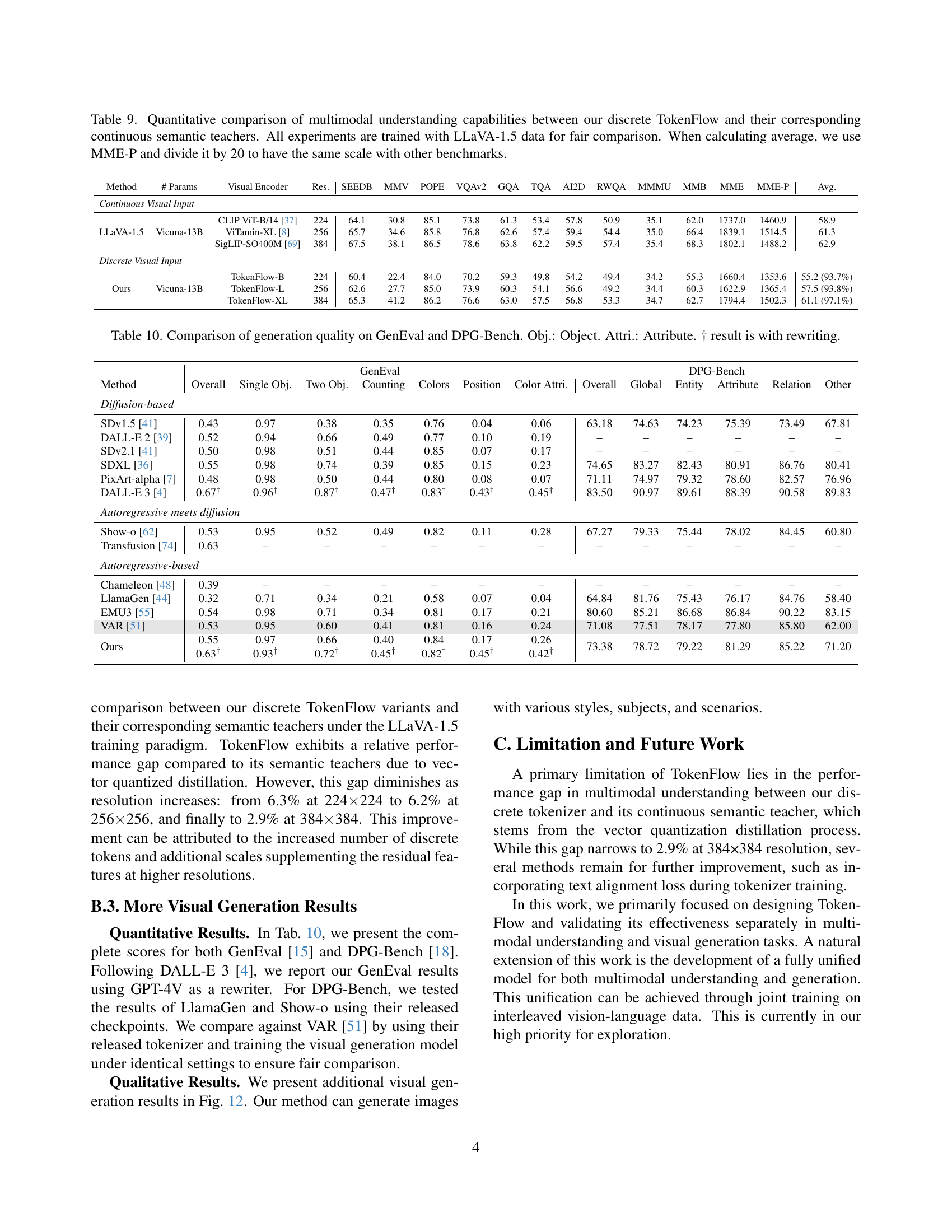
🔼 This table quantitatively compares the performance of TokenFlow (a discrete visual tokenizer) against its continuous semantic teacher models on various multimodal understanding benchmarks. The comparison highlights the performance difference between discrete and continuous visual representations in multimodal understanding tasks. All models were trained using the same LLaVA-1.5 dataset for a fair comparison. The average score is calculated by dividing the MME-P score by 20 to maintain consistency with other benchmarks.
read the caption
Table 9: Quantitative comparison of multimodal understanding capabilities between our discrete TokenFlow and their corresponding continuous semantic teachers. All experiments are trained with LLaVA-1.5 data for fair comparison. When calculating average, we use MME-P and divide it by 20 to have the same scale with other benchmarks.
| Method | GenEval Overall | Single Obj. | Two Obj. | Counting | Colors | Position | Color Attri. | DPG-Bench Overall | Global | Entity | Attribute | Relation | Other |
|---|---|---|---|---|---|---|---|---|---|---|---|---|---|
| Diffusion-based | |||||||||||||
| SDv1.5 [41] | 0.43 | 0.97 | 0.38 | 0.35 | 0.76 | 0.04 | 0.06 | 63.18 | 74.63 | 74.23 | 75.39 | 73.49 | 67.81 |
| DALL-E 2 [39] | 0.52 | 0.94 | 0.66 | 0.49 | 0.77 | 0.10 | 0.19 | – | – | – | – | – | – |
| SDv2.1 [41] | 0.50 | 0.98 | 0.51 | 0.44 | 0.85 | 0.07 | 0.17 | – | – | – | – | – | – |
| SDXL [36] | 0.55 | 0.98 | 0.74 | 0.39 | 0.85 | 0.15 | 0.23 | 74.65 | 83.27 | 82.43 | 80.91 | 86.76 | 80.41 |
| PixArt-alpha [7] | 0.48 | 0.98 | 0.50 | 0.44 | 0.80 | 0.08 | 0.07 | 71.11 | 74.97 | 79.32 | 78.60 | 82.57 | 76.96 |
| DALL-E 3 [4] | 0.67† | 0.96† | 0.87† | 0.47† | 0.83† | 0.43† | 0.45† | 83.50 | 90.97 | 89.61 | 88.39 | 90.58 | 89.83 |
| Autoregressive meets diffusion | |||||||||||||
| Show-o [62] | 0.53 | 0.95 | 0.52 | 0.49 | 0.82 | 0.11 | 0.28 | 67.27 | 79.33 | 75.44 | 78.02 | 84.45 | 60.80 |
| Transfusion [74] | 0.63 | – | – | – | – | – | – | – | – | – | – | – | – |
| Autoregressive-based | |||||||||||||
| Chameleon [48] | 0.39 | – | – | – | – | – | – | – | – | – | – | – | – |
| LlamaGen [44] | 0.32 | 0.71 | 0.34 | 0.21 | 0.58 | 0.07 | 0.04 | 64.84 | 81.76 | 75.43 | 76.17 | 84.76 | 58.40 |
| EMU3 [55] | 0.54 | 0.98 | 0.71 | 0.34 | 0.81 | 0.17 | 0.21 | 80.60 | 85.21 | 86.68 | 86.84 | 90.22 | 83.15 |
| VAR [51] | 0.53 | 0.95 | 0.60 | 0.41 | 0.81 | 0.16 | 0.24 | 71.08 | 77.51 | 78.17 | 77.80 | 85.80 | 62.00 |
| Ours | 0.55 | 0.97 | 0.66 | 0.40 | 0.84 | 0.17 | 0.26 | 73.38 | 78.72 | 79.22 | 81.29 | 85.22 | 71.20 |
| 0.63† | 0.93† | 0.72† | 0.45† | 0.82† | 0.45† | 0.42† |
🔼 This table compares the visual generation capabilities of different models using two metrics: GenEval and DPG-Bench. GenEval assesses overall generation quality, while DPG-Bench breaks down the quality into several sub-categories, including object detection, attribute identification, counting, color accuracy, and positional accuracy. The results show how well each model performs on various aspects of generating coherent and realistic images. The symbol † indicates results achieved using a text rewriting technique to enhance the model’s capabilities.
read the caption
Table 10: Comparison of generation quality on GenEval and DPG-Bench. Obj.: Object. Attri.: Attribute. ††\dagger† result is with rewriting.
| Tokenizer | TokenFlow-B | TokenFlow-L | TokenFlow-XL |
|---|---|---|---|
| Tokenizer settings: | |||
| Input resolution | 224 | 256 | 384 |
| Codebook size | 32,768 | 32,768 | 32,768 |
| Semantic teacher | CLIP ViT-B/14-224 [37] | ViTamin-XL-256 [8] | SigLIP-SO400M-patch14-384 [69] |
| Multi-scale settings | [1, 2, 4, 6, 8, 10, 12, 14] | [1, 2, 3, 4, 6, 8, 10, 12, 14, 16] | [1, 2, 3, 4, 5, 6, 7, 8, 9, 10, 12, 14, 17, 22, 27] |
| Semantic codebook embedding dimension | 32 | 32 | 32 |
| Pixel codebook embedding dimension | 8 | 8 | 8 |
| Training settings: | |||
| Learning rate | 1e-4 | 1e-4 | 1e-4 |
| Batch size | 256 | 256 | 256 |
| Training steps | 1,000,000 | 500,000 | 500,000 |
| Distance balance weight $w_{dis}$ | 1.0 | 1.0 | 1.0 |
| Commitment loss factor $\beta$ | 0.25 | 0.25 | 0.25 |
| Adversarial loss factor $\lambda_{G}$ | 0.5 | 0.5 | 0.5 |
| Max gradient norm | 1.0 | 1.0 | 1.0 |
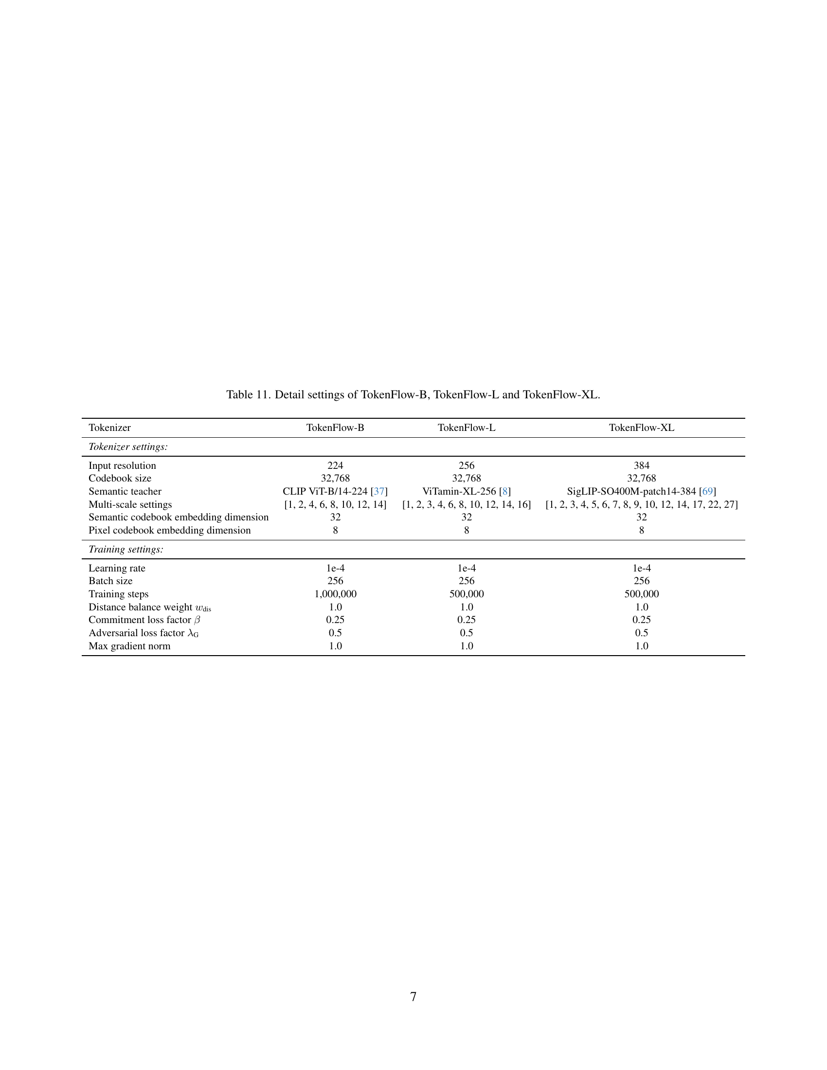
🔼 This table details the specific hyperparameters used during the training of three different versions of the TokenFlow model: TokenFlow-B, TokenFlow-L, and TokenFlow-XL. The table shows the differences in input resolution, codebook size, semantic teacher model used for initialization, multi-scale settings (number of scales and dimensions), pixel codebook embedding dimension, and training settings (learning rate, batch size, number of training steps, distance balance weight, commitment loss factor, adversarial loss factor, and maximum gradient norm). These variations in hyperparameters were made to explore the impact of different training strategies on model performance.
read the caption
Table 11: Detail settings of TokenFlow-B, TokenFlow-L and TokenFlow-XL.
Full paper#
