↗ arXiv ↗ Hugging Face ↗ Papers with Code
TL;DR#
Autonomous vehicles rely heavily on LiDAR for perception, but raw LiDAR data is often sparse, especially in complex scenes. Existing diffusion models can produce high-quality completed scenes but are computationally expensive, hindering real-time applications. This creates a critical need for methods that balance speed and accuracy.
This research introduces ScoreLiDAR, a novel distillation method designed to accelerate the LiDAR scene completion process. ScoreLiDAR leverages a pre-trained diffusion model and incorporates a Structural Loss to ensure high-quality outputs. The results demonstrate a significant speedup (over 5x) without compromising accuracy, paving the way for real-time, accurate scene understanding in autonomous systems.
Key Takeaways#
Why does it matter?#
This paper is crucial for researchers in autonomous driving and 3D computer vision. It addresses the critical need for efficient and high-quality 3D LiDAR scene completion, a vital step in enabling self-driving cars to accurately perceive their surroundings. The proposed method, ScoreLiDAR, offers a significant speedup compared to existing techniques while maintaining accuracy, directly impacting the development of real-time perception systems. This opens avenues for exploring faster diffusion models and improving the robustness of 3D scene understanding in challenging environments.
Visual Insights#

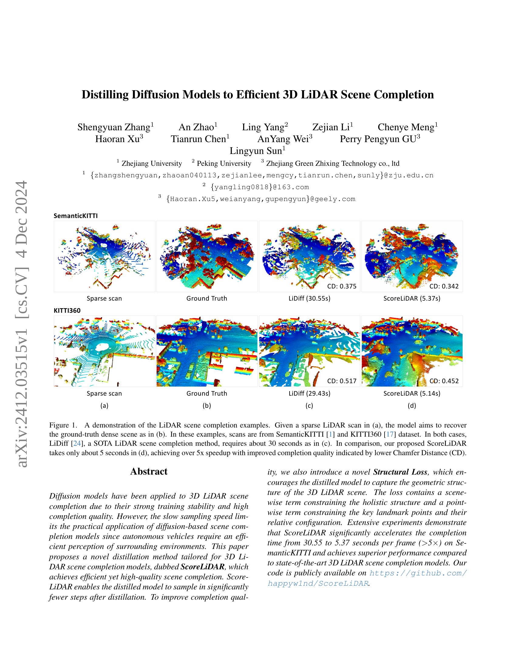
🔼 This figure demonstrates the LiDAR scene completion capabilities of the proposed ScoreLiDAR model and compares it to the state-of-the-art LiDiff model. Subfigure (a) shows a sparse LiDAR scan as input. The model’s goal is to reconstruct the ground-truth dense LiDAR scan shown in (b). (c) presents the results from the LiDiff model, illustrating that it takes approximately 30 seconds to generate a completion. In contrast, (d) displays the significantly faster ScoreLiDAR results, which are generated in roughly 5 seconds. The visual improvement in the completion and the 5x speedup highlight ScoreLiDAR’s efficiency. The Chamfer Distance (CD) metric quantifies the difference between the generated completion and the ground truth, with lower values indicating better quality.
read the caption
Figure 1: A demonstration of the LiDAR scene completion examples. Given a sparse LiDAR scan in (a), the model aims to recover the ground-truth dense scene as in (b). In these examples, scans are from SemanticKITTI [1] and KITTI360 [17] dataset. In both cases, LiDiff [24], a SOTA LiDAR scene completion method, requires about 30 seconds as in (c). In comparison, our proposed ScoreLiDAR takes only about 5 seconds in (d), achieving over 5x speedup with improved completion quality indicated by lower Chamfer Distance (CD).
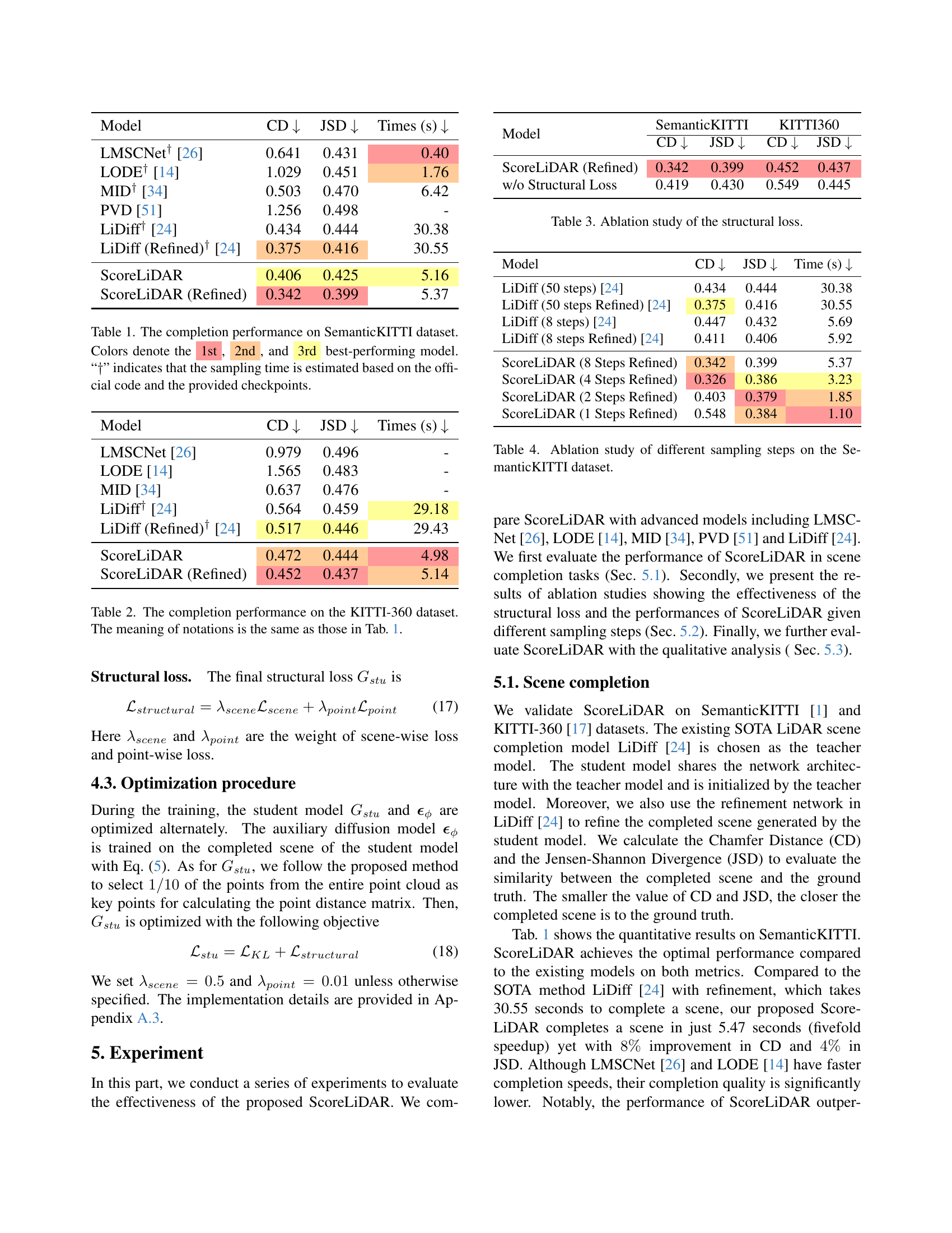
| Model | CD ↓ | JSD ↓ | Times (s) ↓ |
|---|---|---|---|
| LMSCNet† [26] | 0.641 | 0.431 | 0.40 |
| LODE† [14] | 1.029 | 0.451 | 1.76 |
| MID† [34] | 0.503 | 0.470 | 6.42 |
| PVD [51] | 1.256 | 0.498 | - |
| LiDiff† [24] | 0.434 | 0.444 | 30.38 |
| LiDiff (Refined)† [24] | 0.375 | 0.416 | 30.55 |
| ScoreLiDAR | 0.406 | 0.425 | 5.16 |
| ScoreLiDAR (Refined) | 0.342 | 0.399 | 5.37 |
🔼 This table presents a quantitative comparison of different 3D LiDAR scene completion models on the SemanticKITTI dataset. The models are evaluated using two metrics: Chamfer Distance (CD), measuring the geometric difference between the completed scene and the ground truth, and Jensen-Shannon Divergence (JSD), assessing the similarity of probability distributions of point clouds. Lower values for both metrics indicate better completion quality. The table also reports the completion time for each model. Note that the time for some models is an estimate based on publicly available code and checkpoints rather than direct runtime measurement.
read the caption
Table 1: The completion performance on SemanticKITTI dataset. Colors denote the 1st, 2nd, and 3rd best-performing model. “††{\dagger}†” indicates that the sampling time is estimated based on the official code and the provided checkpoints.
In-depth insights#
Diffusion Model Distillation#
Diffusion model distillation, in the context of 3D LiDAR scene completion, presents a powerful technique to enhance efficiency without sacrificing quality. The core idea revolves around training a smaller, faster “student” model to mimic the behavior of a larger, slower, but more accurate “teacher” diffusion model. This approach leverages the teacher’s learned representations to guide the student’s training, resulting in a significant speedup during inference. Key to success is carefully designing the distillation loss function, ensuring the student accurately replicates the teacher’s output while minimizing computational cost. Furthermore, incorporating structural losses further refines the student model’s understanding of geometric features, leading to improved completion quality. This distillation method, therefore, is crucial for deploying diffusion models in real-time applications like autonomous driving, where speed and accuracy are paramount. The technique shows promise in bridging the gap between powerful but computationally expensive models and the practical demands of resource-constrained environments.
Structural Loss#
The paper introduces a novel ‘Structural Loss’ to improve the quality of 3D LiDAR scene completion. This loss function addresses limitations of existing diffusion models which sometimes struggle with preserving fine details and geometric accuracy in the completed scenes. It’s a two-pronged approach: a scene-wise term constrains the overall holistic structure of the completed scene, ensuring it aligns with the global shape of the ground truth. Simultaneously, a point-wise term focuses on key landmark points and their relative configurations within the scene, ensuring local geometric accuracy. By combining these terms, the Structural Loss guides the student model to capture both macroscopic and microscopic features of the 3D scene, resulting in higher fidelity and more realistic completions. This is especially important for autonomous vehicle applications where accurate perception of surroundings is critical. The effectiveness of the Structural Loss is demonstrated through ablation studies, showing a significant improvement in completion quality compared to models without it. This showcases the importance of explicitly incorporating geometric constraints during the distillation process, leading to more accurate and efficient 3D LiDAR scene completion.
Speed-Quality Tradeoff#
The concept of a speed-quality tradeoff is central to evaluating the efficiency and effectiveness of 3D LiDAR scene completion models. ScoreLiDAR directly addresses this tradeoff, offering a compelling solution to the inherent conflict between computational speed and the quality of the completed scene. Traditional diffusion models, while achieving high quality, suffer from slow inference times, making them impractical for real-time applications. ScoreLiDAR leverages a distillation technique to significantly reduce inference time, achieving a 5x speedup while maintaining superior quality to existing methods. This improvement results from both the distillation process itself and the introduction of a novel Structural Loss, which helps the model capture geometric details that are often lost with faster methods. The results highlight ScoreLiDAR’s ability to achieve a significantly better balance between speed and quality, ultimately enhancing its suitability for deployment in autonomous driving and similar applications where fast, accurate scene understanding is crucial.
Future Research#
Future research directions for ScoreLiDAR should prioritize improving the robustness of the model against various noise levels and data sparsity. This could involve exploring alternative distillation methods or incorporating advanced noise modeling techniques. Additionally, investigating the impact of different network architectures and loss functions on the model’s performance is crucial. Further exploration into handling complex geometric structures, especially in the presence of occlusion, is necessary. Addressing the over-completion issue observed in some instances should be a key focus. This may involve refining the structural loss or developing novel regularization techniques. Finally, extending the capabilities of ScoreLiDAR to incorporate semantic information and perform semantic scene completion is a significant avenue to explore, which would increase the model’s applicability in autonomous driving applications.
Limitations#
The authors acknowledge key limitations of ScoreLiDAR, primarily stemming from its reliance on a teacher model. Performance is inherently bound by the teacher model’s capabilities, meaning improvements in the teacher directly translate to ScoreLiDAR improvements but not exceeding them. The ability to perform semantic scene completion is also limited by the teacher’s ability. If the teacher model lacks semantic understanding, ScoreLiDAR will inherit this limitation. Future work should focus on mitigating this dependency, potentially exploring alternative training methods or architectural changes to allow ScoreLiDAR to surpass the teacher and handle semantic tasks more effectively. Another area for improvement is to address situations of over-completion, where the model adds details or structure not present in the ground truth. This issue likely stems from the data augmentation method used during training, where the number of points is artificially inflated. Further research could focus on refining this process to better control the balance between accuracy and efficiency. Addressing these limitations would make ScoreLiDAR a more robust and independent scene completion solution.
More visual insights#
More on figures
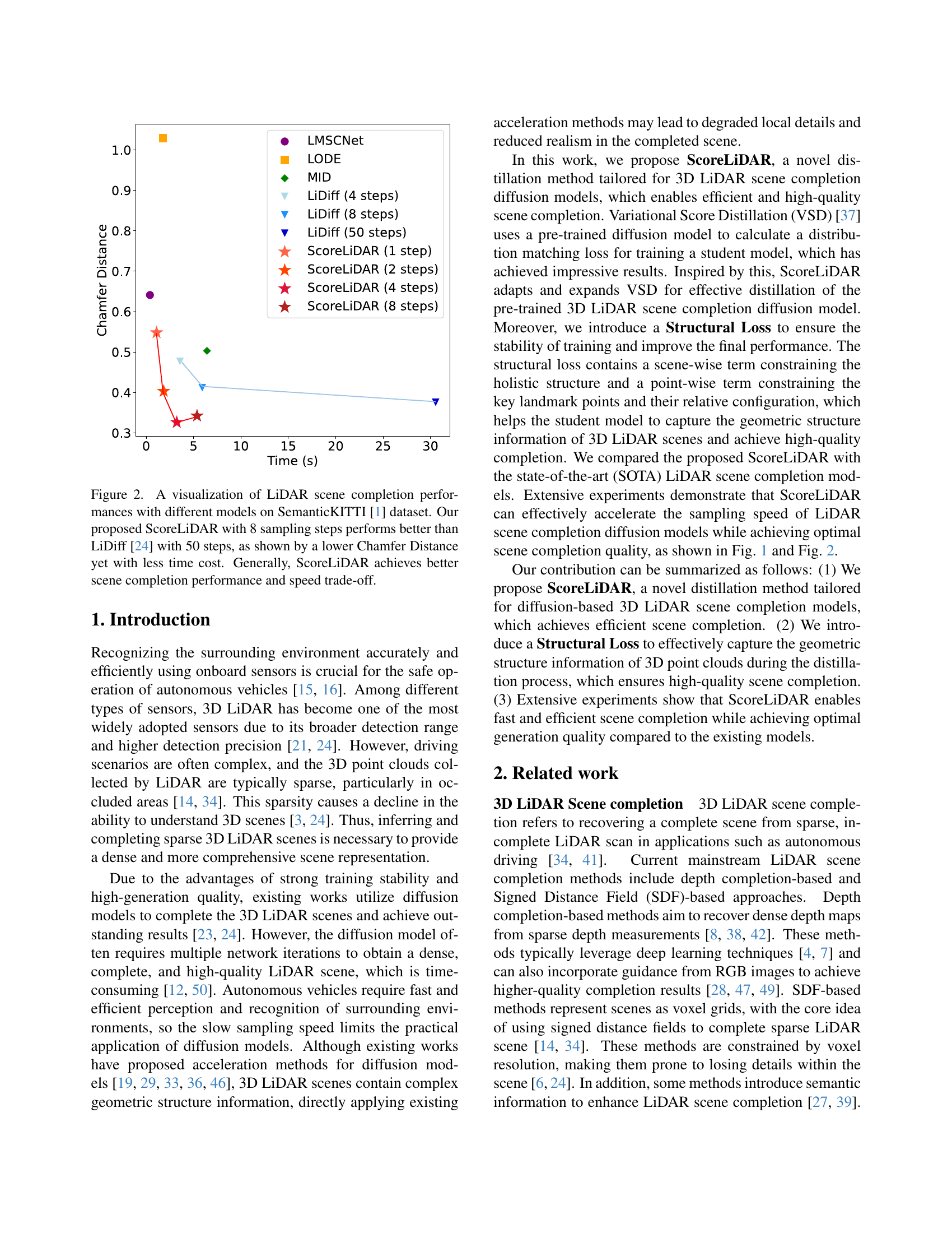
🔼 This figure compares the performance of different LiDAR scene completion models on the SemanticKITTI dataset. The y-axis represents the Chamfer Distance (CD), a metric that measures the difference between a completed LiDAR scan and the ground truth. The x-axis shows the time taken to complete the scan. Each point represents a model with a specified number of sampling steps. The figure shows that ScoreLiDAR, with only 8 sampling steps, achieves a lower CD (better quality) than LiDiff (a state-of-the-art method) with 50 steps. Moreover, ScoreLiDAR is significantly faster. This demonstrates the efficiency and effectiveness of the ScoreLiDAR model.
read the caption
Figure 2: A visualization of LiDAR scene completion performances with different models on SemanticKITTI [1] dataset. Our proposed ScoreLiDAR with 8 sampling steps performs better than LiDiff [24] with 50 steps, as shown by a lower Chamfer Distance yet with less time cost. Generally, ScoreLiDAR achieves better scene completion performance and speed trade-off.

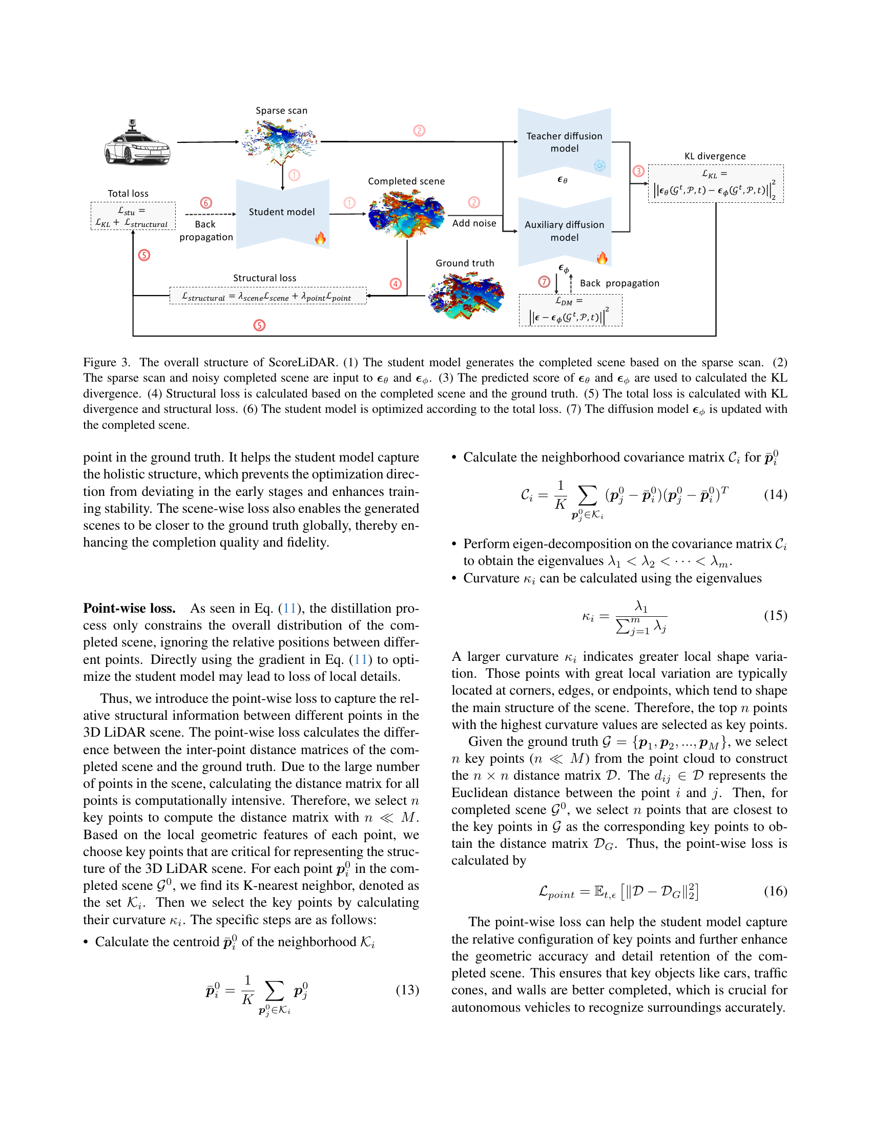
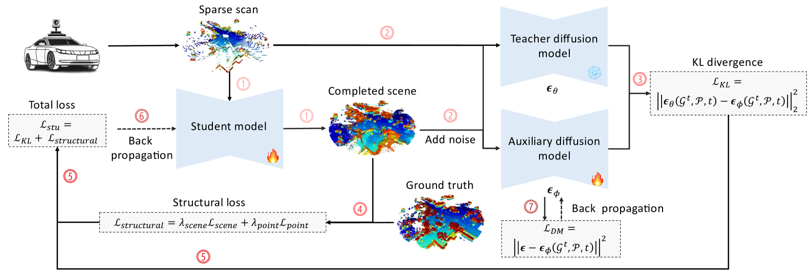
🔼 This figure illustrates the ScoreLiDAR framework, detailing a novel distillation method for efficient 3D LiDAR scene completion. The process starts with a student model generating a completed scene from a sparse LiDAR scan. Simultaneously, a teacher model (ϵθ) and an auxiliary diffusion model (ϵϕ) process the sparse scan and the noisy completed scene to compute a KL divergence loss, measuring the difference between their predicted scores. A structural loss is also calculated, comparing the completed scene to the ground truth. These two losses are combined to form a total loss that optimizes the student model. Finally, the auxiliary model (ϵϕ) is updated using the completed scene, refining its performance for future iterations.
read the caption
Figure 3: The overall structure of ScoreLiDAR. (1) The student model generates the completed scene based on the sparse scan. (2) The sparse scan and noisy completed scene are input to ϵθsubscriptbold-italic-ϵ𝜃\boldsymbol{\epsilon}_{\theta}bold_italic_ϵ start_POSTSUBSCRIPT italic_θ end_POSTSUBSCRIPT and ϵϕsubscriptbold-italic-ϵitalic-ϕ\boldsymbol{\epsilon}_{\phi}bold_italic_ϵ start_POSTSUBSCRIPT italic_ϕ end_POSTSUBSCRIPT. (3) The predicted score of ϵθsubscriptbold-italic-ϵ𝜃\boldsymbol{\epsilon}_{\theta}bold_italic_ϵ start_POSTSUBSCRIPT italic_θ end_POSTSUBSCRIPT and ϵϕsubscriptbold-italic-ϵitalic-ϕ\boldsymbol{\epsilon}_{\phi}bold_italic_ϵ start_POSTSUBSCRIPT italic_ϕ end_POSTSUBSCRIPT are used to calculated the KL divergence. (4) Structural loss is calculated based on the completed scene and the ground truth. (5) The total loss is calculated with KL divergence and structural loss. (6) The student model is optimized according to the total loss. (7) The diffusion model ϵϕsubscriptbold-italic-ϵitalic-ϕ\boldsymbol{\epsilon}_{\phi}bold_italic_ϵ start_POSTSUBSCRIPT italic_ϕ end_POSTSUBSCRIPT is updated with the completed scene.

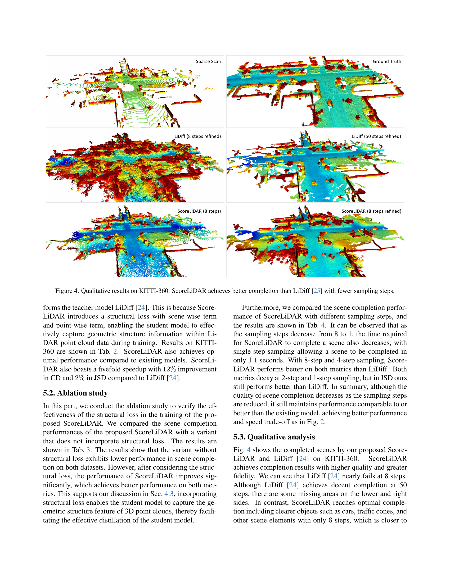
🔼 Figure 4 presents a qualitative comparison of 3D LiDAR scene completion results on the KITTI-360 dataset. It visually demonstrates the performance of the proposed ScoreLiDAR method against the state-of-the-art LiDiff method. The figure shows the input sparse LiDAR scan, the ground truth dense LiDAR scan, and the completed scans generated by both methods. By comparing the visual quality of the completed scans, it’s evident that ScoreLiDAR achieves better scene completion, particularly in terms of detail and accuracy, even with significantly fewer sampling steps than LiDiff. This highlights the efficiency and effectiveness of the ScoreLiDAR model.
read the caption
Figure 4: Qualitative results on KITTI-360. ScoreLiDAR achieves better completion than LiDiff [25] with fewer sampling steps.

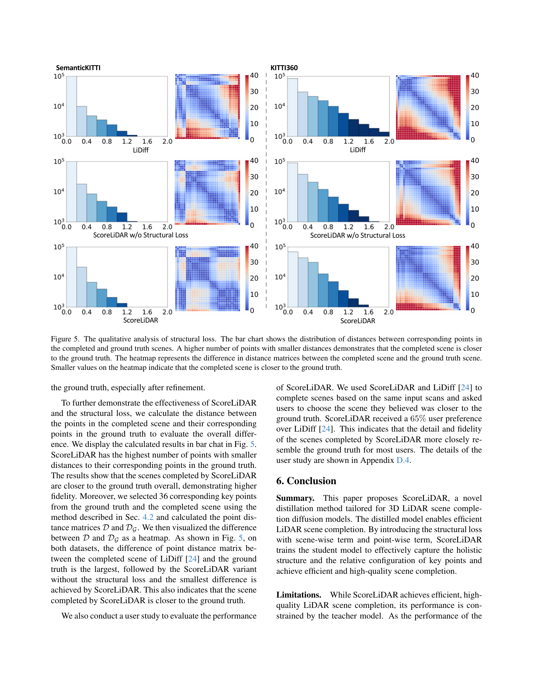
🔼 This figure presents a qualitative analysis of the impact of the structural loss on 3D LiDAR scene completion. It uses two visualizations to demonstrate this impact: (1) a bar chart showing the distribution of distances between corresponding points in the completed and ground truth scenes. This chart highlights that a greater number of points with smaller distances implies higher fidelity (i.e., closer similarity to the ground truth). (2) a heatmap visualizing the difference between the distance matrices for the completed and ground truth scenes. Smaller values in this heatmap correspond to a closer resemblance between the completed and ground truth scenes, again indicating better completion quality.
read the caption
Figure 5: The qualitative analysis of structural loss. The bar chart shows the distribution of distances between corresponding points in the completed and ground truth scenes. A higher number of points with smaller distances demonstrates that the completed scene is closer to the ground truth. The heatmap represents the difference in distance matrices between the completed scene and the ground truth scene. Smaller values on the heatmap indicate that the completed scene is closer to the ground truth.

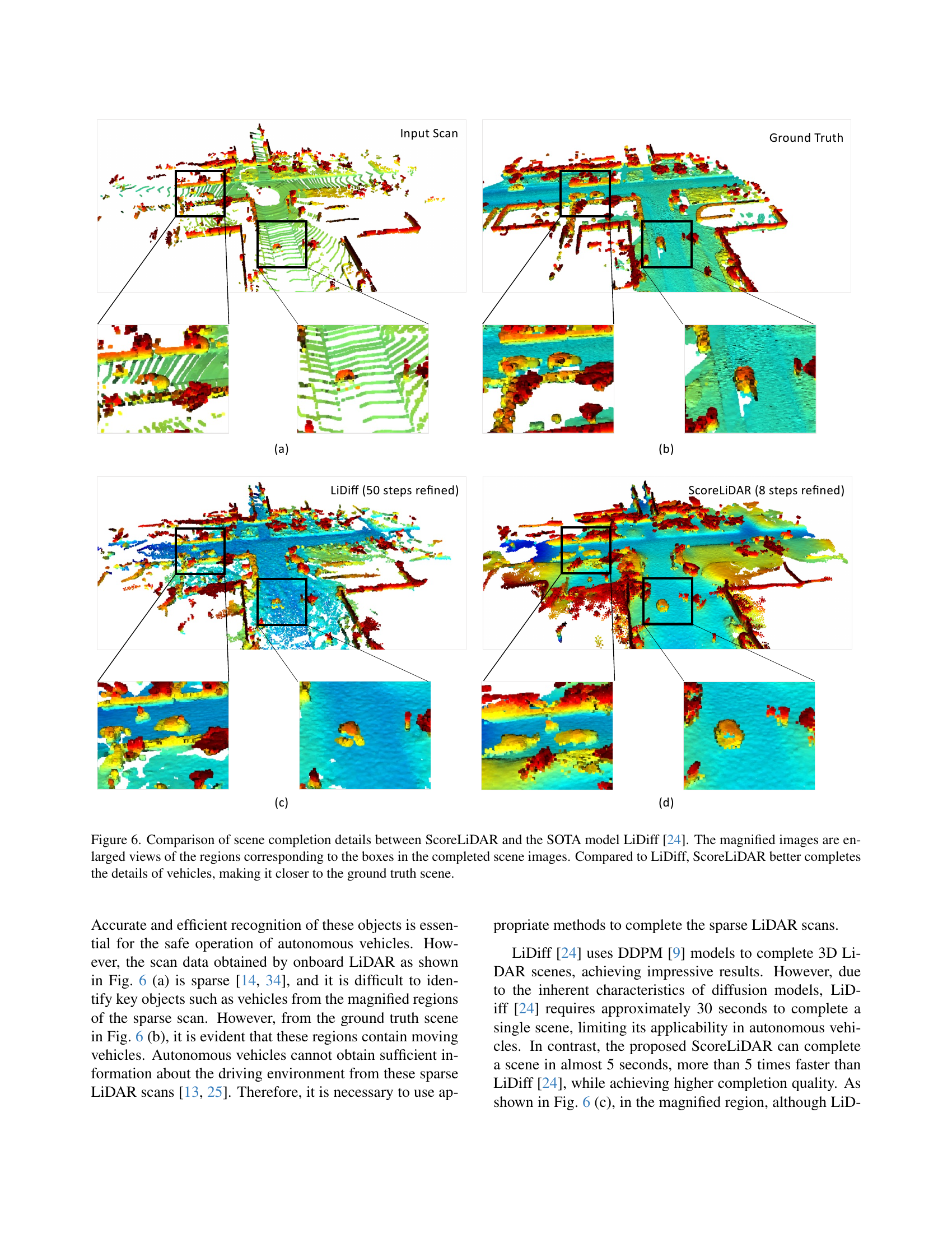
🔼 Figure 6 presents a detailed comparison of scene completion results between ScoreLiDAR and LiDiff, a state-of-the-art method. The figure shows both the overall completed scenes and zoomed-in sections highlighting key areas (indicated by boxes). The zoomed-in views directly compare the fine details of completed vehicle models produced by each method. The comparison demonstrates that ScoreLiDAR achieves more accurate and realistic completion of vehicles and their surrounding details, resulting in a completed scene that is closer to the ground truth.
read the caption
Figure 6: Comparison of scene completion details between ScoreLiDAR and the SOTA model LiDiff [24]. The magnified images are enlarged views of the regions corresponding to the boxes in the completed scene images. Compared to LiDiff, ScoreLiDAR better completes the details of vehicles, making it closer to the ground truth scene.

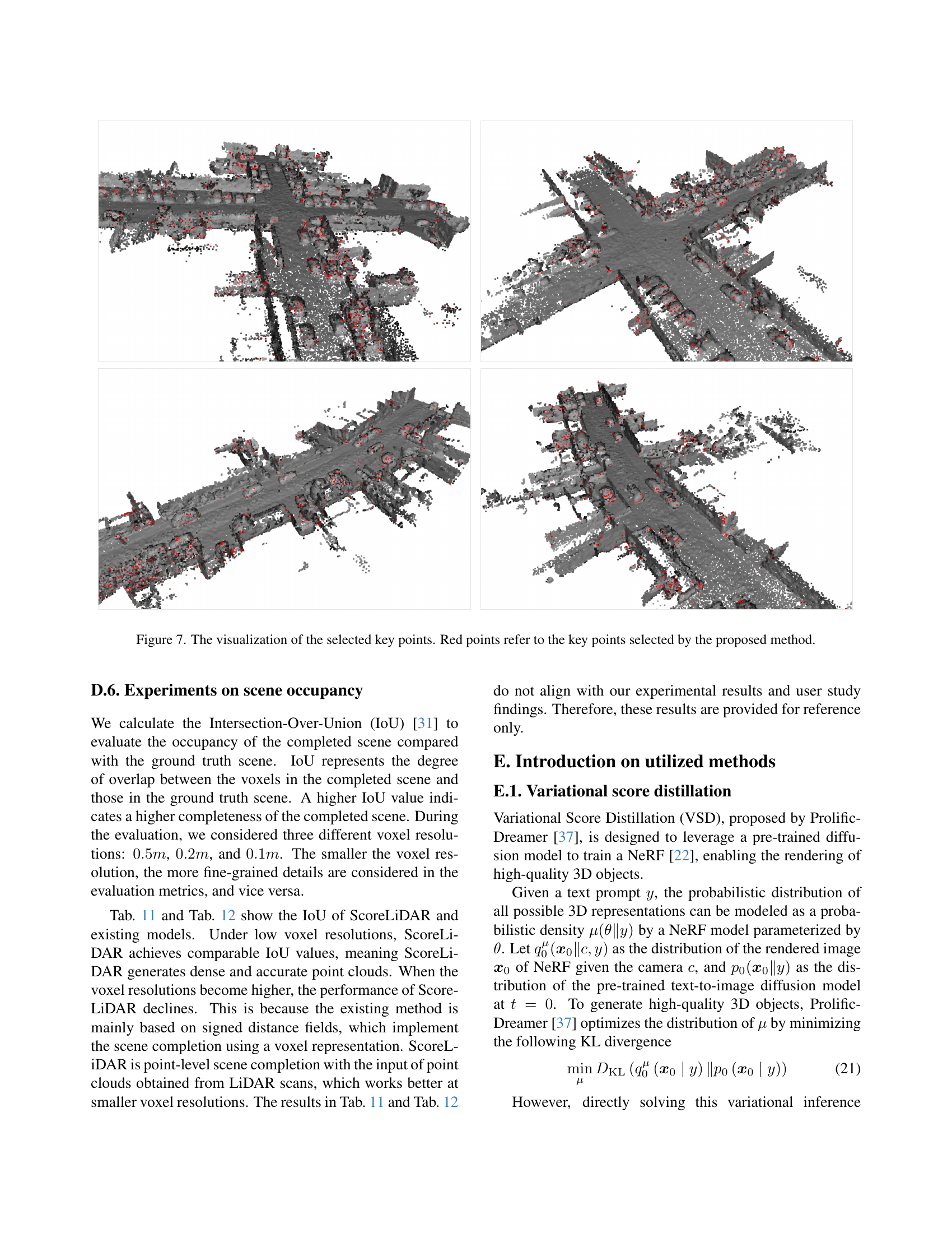
🔼 This figure visualizes the key points selected by the proposed ScoreLiDAR method for 3D LiDAR scene completion. The red points highlight the key points chosen by the algorithm. These points are strategically selected based on local geometric features to effectively capture the structural information of the scene. By focusing on these key points, the method improves the accuracy and efficiency of the scene completion process. The figure shows several example scenes where the chosen key points are marked in red.
read the caption
Figure 7: The visualization of the selected key points. Red points refer to the key points selected by the proposed method.

🔼 This figure showcases several examples of 3D LiDAR scene completion using the ScoreLiDAR model on the KITTI-360 dataset. Each row presents a pair of images: the left image displays the incomplete sparse LiDAR scan, while the right image shows the corresponding ground truth dense scene. Below them, two more images are displayed showing the scene completion results: first with LiDiff, a state-of-the-art LiDAR scene completion method for comparison, and then with the ScoreLiDAR model. The results demonstrate ScoreLiDAR’s ability to produce high-quality, complete scenes similar to the ground truth, even with fewer sampling steps, leading to significant time savings.
read the caption
Figure 8: Completed samples of ScoreLiDAR from KITTI-360 dataset.

🔼 Figure 9 presents a visual comparison of 3D LiDAR scene completion results using the proposed ScoreLiDAR method against the ground truth. It showcases four pairs of completed scenes, each with a corresponding input (sparse) scan and the ground truth dense scene. Each row shows a different scenario, highlighting the ability of ScoreLiDAR to reconstruct missing parts of the scene from limited input data. This figure helps to visually demonstrate the performance and capabilities of ScoreLiDAR in the context of 3D LiDAR scene completion, focusing on its efficiency and ability to handle the sparsity typical of LiDAR data.
read the caption
Figure 9: Completed samples of ScoreLiDAR from SemanticKITTI dataset.
More on tables
| Model | CD ↓ | JSD ↓ | Times (s) ↓ |
|---|---|---|---|
| LMSCNet [26] | 0.979 | 0.496 | - |
| LODE [14] | 1.565 | 0.483 | - |
| MID [34] | 0.637 | 0.476 | - |
| LiDiff † [24] | 0.564 | 0.459 | 29.18 |
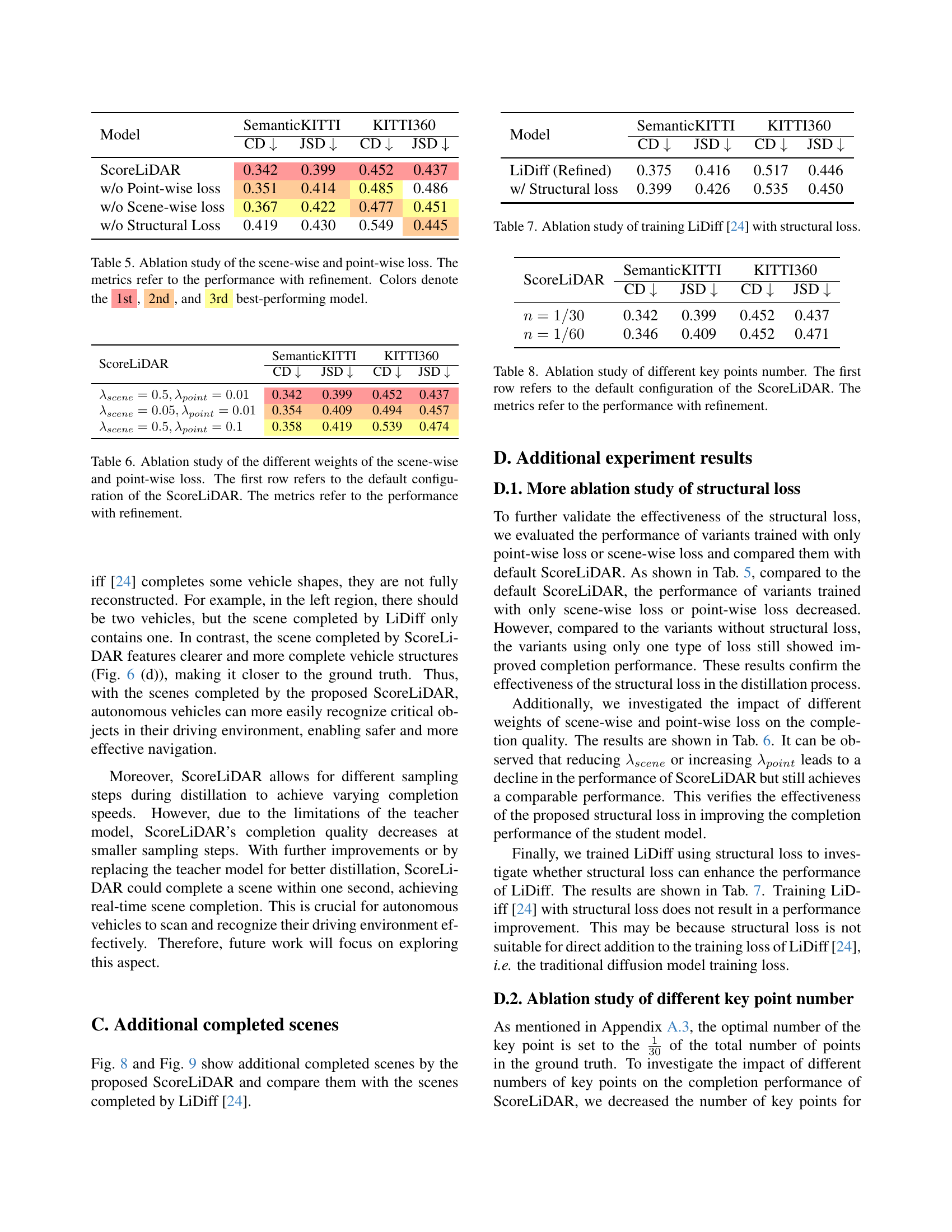
| LiDiff (Refined) † [24] | 0.517 | 0.446 | 29.43 |
| ScoreLiDAR | 0.472 | 0.444 | 4.98 |
| ScoreLiDAR (Refined) | 0.452 | 0.437 | 5.14 |
🔼 This table presents a quantitative evaluation of different methods for 3D LiDAR scene completion on the KITTI-360 dataset. It shows the Chamfer Distance (CD) and Jensen-Shannon Divergence (JSD) scores achieved by various models. Lower CD and JSD values indicate better scene completion quality. The results allow for a comparison of the accuracy and fidelity of different approaches to reconstructing a complete 3D LiDAR scene from sparse input data.
read the caption
Table 2: The completion performance on the KITTI-360 dataset. The meaning of notations is the same as those in Tab. 1.
| Model | SemanticKITTI CD ↓ | SemanticKITTI JSD ↓ | KITTI360 CD ↓ | KITTI360 JSD ↓ |
|---|---|---|---|---|
| ScoreLiDAR (Refined) | 0.342 | 0.399 | 0.452 | 0.437 |
| w/o Structural Loss | 0.419 | 0.430 | 0.549 | 0.445 |
🔼 This table presents an ablation study to evaluate the impact of the proposed structural loss on the performance of the ScoreLiDAR model. It compares the results of ScoreLiDAR with and without the structural loss, showing the improvements in terms of Chamfer Distance (CD) and Jensen-Shannon Divergence (JSD) on both the SemanticKITTI and KITTI360 datasets. Lower CD and JSD values indicate better scene completion quality.
read the caption
Table 3: Ablation study of the structural loss.
| Model | CD ↓ | JSD ↓ | Time (s) ↓ |
|---|---|---|---|
| LiDiff (50 steps) [24] | 0.434 | 0.444 | 30.38 |
| LiDiff (50 steps Refined) [24] | 0.375 | 0.416 | 30.55 |
| LiDiff (8 steps) [24] | 0.447 | 0.432 | 5.69 |
| LiDiff (8 steps Refined) [24] | 0.411 | 0.406 | 5.92 |
| ScoreLiDAR (8 Steps Refined) | 0.342 | 0.399 | 5.37 |
| ScoreLiDAR (4 Steps Refined) | 0.326 | 0.386 | 3.23 |
| ScoreLiDAR (2 Steps Refined) | 0.403 | 0.379 | 1.85 |
| ScoreLiDAR (1 Steps Refined) | 0.548 | 0.384 | 1.10 |
🔼 This table presents the results of an ablation study conducted to analyze the effect of varying the number of sampling steps in the ScoreLiDAR model on the SemanticKITTI dataset. The study measures the performance of the model with different numbers of sampling steps (1, 2, 4, and 8 steps), and also includes results for a refined version of the model. The metrics used to evaluate performance are Chamfer Distance (CD) and Jensen-Shannon Divergence (JSD), which both measure the difference between the completed point clouds produced by the model and the ground truth point clouds. Lower values of CD and JSD indicate better completion quality.
read the caption
Table 4: Ablation study of different sampling steps on the SemanticKITTI dataset.
| Model | SemanticKITTI CD ↓ | SemanticKITTI JSD ↓ | KITTI360 CD ↓ | KITTI360 JSD ↓ |
|---|---|---|---|---|
| ScoreLiDAR | 0.342 | 0.399 | 0.452 | 0.437 |
| w/o Point-wise loss | 0.351 | 0.414 | 0.485 | 0.486 |
| w/o Scene-wise loss | 0.367 | 0.422 | 0.477 | 0.451 |
| w/o Structural Loss | 0.419 | 0.430 | 0.549 | 0.445 |
🔼 This table presents an ablation study evaluating the impact of the scene-wise and point-wise loss components within the ScoreLiDAR model. The results show the model’s performance (using Chamfer Distance and Jensen-Shannon Divergence metrics) on the SemanticKITTI and KITTI360 datasets, both with and without these loss components, as well as the overall model. The refinement process was applied to all results. Color-coding highlights the top three performing configurations based on the combined metrics.
read the caption
Table 5: Ablation study of the scene-wise and point-wise loss. The metrics refer to the performance with refinement. Colors denote the 1st, 2nd, and 3rd best-performing model.
| ScoreLiDAR | SemanticKITTI | KITTI360 | ||
|---|---|---|---|---|
| CD ↓ | JSD ↓ | CD ↓ | JSD ↓ | |
| $ | ||||
| \lambda_{scene}=0.5,\lambda_{point}=0.01$ | 0.342 | 0.399 | 0.452 | 0.437 |
| $ | ||||
| \lambda_{scene}=0.05,\lambda_{point}=0.01$ | 0.354 | 0.409 | 0.494 | 0.457 |
| $ | ||||
| \lambda_{scene}=0.5,\lambda_{point}=0.1$ | 0.358 | 0.419 | 0.539 | 0.474 |
🔼 This table presents an ablation study analyzing the impact of varying the weights assigned to the scene-wise and point-wise loss components within the ScoreLiDAR model. The first row shows the performance using the default weights. Subsequent rows illustrate the effect of adjusting these weights, demonstrating the sensitivity of the model to different weighting schemes. All results presented include post-processing refinement steps applied to the generated output. The metrics presented are Chamfer Distance (CD) and Jensen-Shannon Divergence (JSD), lower values indicating better performance.
read the caption
Table 6: Ablation study of the different weights of the scene-wise and point-wise loss. The first row refers to the default configuration of the ScoreLiDAR. The metrics refer to the performance with refinement.
| Model | SemanticKITTI CD ↓ | SemanticKITTI JSD ↓ | KITTI360 CD ↓ | KITTI360 JSD ↓ |
|---|---|---|---|---|
| LiDiff (Refined) | 0.375 | 0.416 | 0.517 | 0.446 |
| w/ Structural loss | 0.399 | 0.426 | 0.535 | 0.450 |
🔼 This table presents the results of an ablation study evaluating the impact of adding a structural loss to the LiDiff model for 3D LiDAR scene completion. It compares the performance of the original LiDiff model (without structural loss) to a version trained with the addition of the structural loss. The comparison uses Chamfer Distance (CD) and Jensen-Shannon Divergence (JSD) as metrics on the SemanticKITTI and KITTI360 datasets to assess the quality of the 3D scene completion.
read the caption
Table 7: Ablation study of training LiDiff [24] with structural loss.
| ScoreLiDAR | SemanticKITTI | KITTI360 | ||
|---|---|---|---|---|
| CD ↓ | JSD ↓ | CD ↓ | JSD ↓ | |
| n=1/30 | 0.342 | 0.399 | 0.452 | 0.437 |
| n=1/60 | 0.346 | 0.409 | 0.452 | 0.471 |
🔼 This table presents an ablation study on the impact of varying the number of key points used in the ScoreLiDAR model. The study investigates how the selection of different numbers of key points affects the model’s performance after refinement. The first row shows the results using the default configuration of the ScoreLiDAR model, while subsequent rows show the performance with reduced numbers of key points. The metrics used to evaluate performance are Chamfer Distance (CD) and Jensen-Shannon Divergence (JSD), both lower values indicating improved accuracy and fidelity compared to the ground truth.
read the caption
Table 8: Ablation study of different key points number. The first row refers to the default configuration of the ScoreLiDAR. The metrics refer to the performance with refinement.
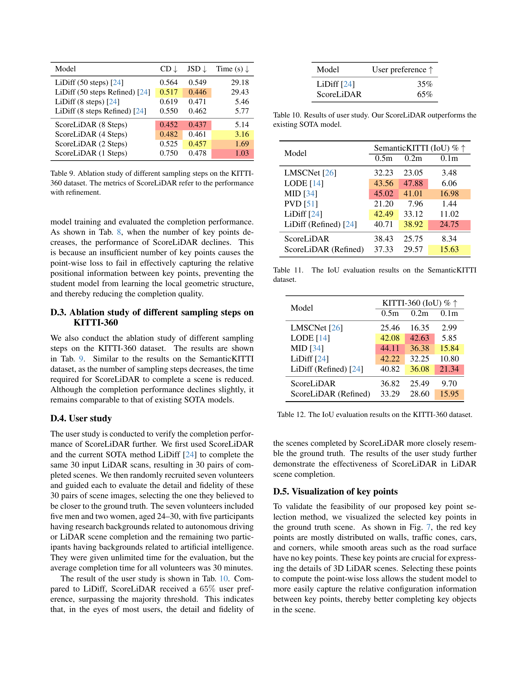
| Model | CD ↓ | JSD ↓ | Time (s) ↓ |
|---|---|---|---|
| LiDiff (50 steps) [24] | 0.564 | 0.549 | 29.18 |
| LiDiff (50 steps Refined) [24] | 0.517 | 0.446 | 29.43 |
| LiDiff (8 steps) [24] | 0.619 | 0.471 | 5.46 |
| LiDiff (8 steps Refined) [24] | 0.550 | 0.462 | 5.77 |
| ScoreLiDAR (8 Steps) | 0.452 | 0.437 | 5.14 |
| ScoreLiDAR (4 Steps) | 0.482 | 0.461 | 3.16 |
| ScoreLiDAR (2 Steps) | 0.525 | 0.457 | 1.69 |
| ScoreLiDAR (1 Steps) | 0.750 | 0.478 | 1.03 |
🔼 This table presents an ablation study analyzing the effect of varying the number of sampling steps on the performance of the ScoreLiDAR model for 3D LiDAR scene completion on the KITTI-360 dataset. It compares the performance of ScoreLiDAR using different numbers of sampling steps (8, 4, 2, and 1) against the baseline LiDiff model with 50 sampling steps. Both the baseline LiDiff model and the ScoreLiDAR models’ performance are measured with and without refinement, showing the impact of refinement on the results. The metrics used for comparison are Chamfer Distance (CD) and Jensen-Shannon Divergence (JSD), lower values indicating better scene completion quality. The ‘Time (s)’ column displays the time taken for scene completion. The results show the trade-off between completion speed and accuracy at various sampling steps.
read the caption
Table 9: Ablation study of different sampling steps on the KITTI-360 dataset. The metrics of ScoreLiDAR refer to the performance with refinement.
| Model | User preference ↑ |
|---|---|
| LiDiff [24] | 35% |
| ScoreLiDAR | 65% |
🔼 A user study was conducted to compare the scene completion quality of ScoreLiDAR and the state-of-the-art (SOTA) LiDiff model. Thirty pairs of completed scenes were generated using both methods for the same 30 input LiDAR scans. Seven volunteers evaluated each pair and selected the one that was more similar to the corresponding ground truth scene. ScoreLiDAR received a 65% user preference over LiDiff, demonstrating its superior performance in producing realistic and accurate scene completions.
read the caption
Table 10: Results of user study. Our ScoreLiDAR outperforms the existing SOTA model.
| Model | SemanticKITTI (IoU) % ↑ | 0.5m | 0.2m | 0.1m |
|---|---|---|---|---|
| LMSCNet [26] | 32.23 | 23.05 | 3.48 | |
| LODE [14] | 43.56 | 47.88 | 6.06 | |
| MID [34] | 45.02 | 41.01 | 16.98 | |
| PVD [51] | 21.20 | 7.96 | 1.44 | |
| LiDiff [24] | 42.49 | 33.12 | 11.02 | |
| LiDiff (Refined) [24] | 40.71 | 38.92 | 24.75 | |
| ScoreLiDAR | 38.43 | 25.75 | 8.34 | |
| ScoreLiDAR (Refined) | 37.33 | 29.57 | 15.63 |
🔼 This table presents the Intersection over Union (IoU) scores achieved by different models on the SemanticKITTI dataset. IoU is a common metric for evaluating the accuracy of semantic segmentation, measuring the overlap between the predicted segmentation and the ground truth. The results are shown for three different voxel resolutions (0.5m, 0.2m, and 0.1m), representing different levels of detail. Higher IoU values indicate better performance.
read the caption
Table 11: The IoU evaluation results on the SemanticKITTI dataset.
| Model | KITTI-360 (IoU) % ↑ | |||
|---|---|---|---|---|
| 0.5m | 0.2m | 0.1m | ||
| LMSCNet [26] | 25.46 | 16.35 | 2.99 | |
| LODE [14] | 42.08 | 42.63 | 5.85 | |
| MID [34] | 44.11 | 36.38 | 15.84 | |
| LiDiff [24] | 42.22 | 32.25 | 10.80 | |
| LiDiff (Refined) [24] | 40.82 | 36.08 | 21.34 | |
| ScoreLiDAR | 36.82 | 25.49 | 9.70 | |
| ScoreLiDAR (Refined) | 33.29 | 28.60 | 15.95 |
🔼 This table presents the Intersection over Union (IoU) scores for different 3D LiDAR scene completion models on the KITTI-360 dataset. IoU is a metric measuring the overlap between the predicted scene and ground truth at various voxel resolutions (0.5m, 0.2m, and 0.1m). Higher IoU values indicate better completion accuracy. The models compared include LMSCNet, LODE, MID, PVD, LiDiff (with and without refinement), and ScoreLiDAR (with and without refinement). The table shows how well each model performs at these different resolutions, allowing for a comparison of completion quality and detail.
read the caption
Table 12: The IoU evaluation results on the KITTI-360 dataset.
Full paper#
