↗ arXiv ↗ Hugging Face ↗ Papers with Code
TL;DR#
Vision-Language Models (VLMs) are crucial for various AI applications but current models often lack versatility and scalability. Existing VLMs frequently underperform on tasks beyond their initial training scope, and scaling models for improved performance can be computationally expensive. Many VLMs are also not publicly available, limiting reproducibility and community collaboration.
PaliGemma 2 addresses these issues by offering a family of open-weight VLMs with varying sizes and resolutions. It systematically studies how these factors affect transfer learning, showing improved performance across a wider range of tasks. This includes novel applications like OCR-related tasks, as well as achieving state-of-the-art results on several benchmarks. The open-weight nature encourages community involvement and further research.
Key Takeaways#
Why does it matter?#
This paper is important because it introduces PaliGemma 2, a family of versatile and open-weight Vision-Language Models (VLMs). This advancement significantly improves transfer learning performance across various tasks and scales, making it highly relevant to current research trends in VLM development. Its open-weight nature fosters further research by providing a valuable resource for the community.
Visual Insights#

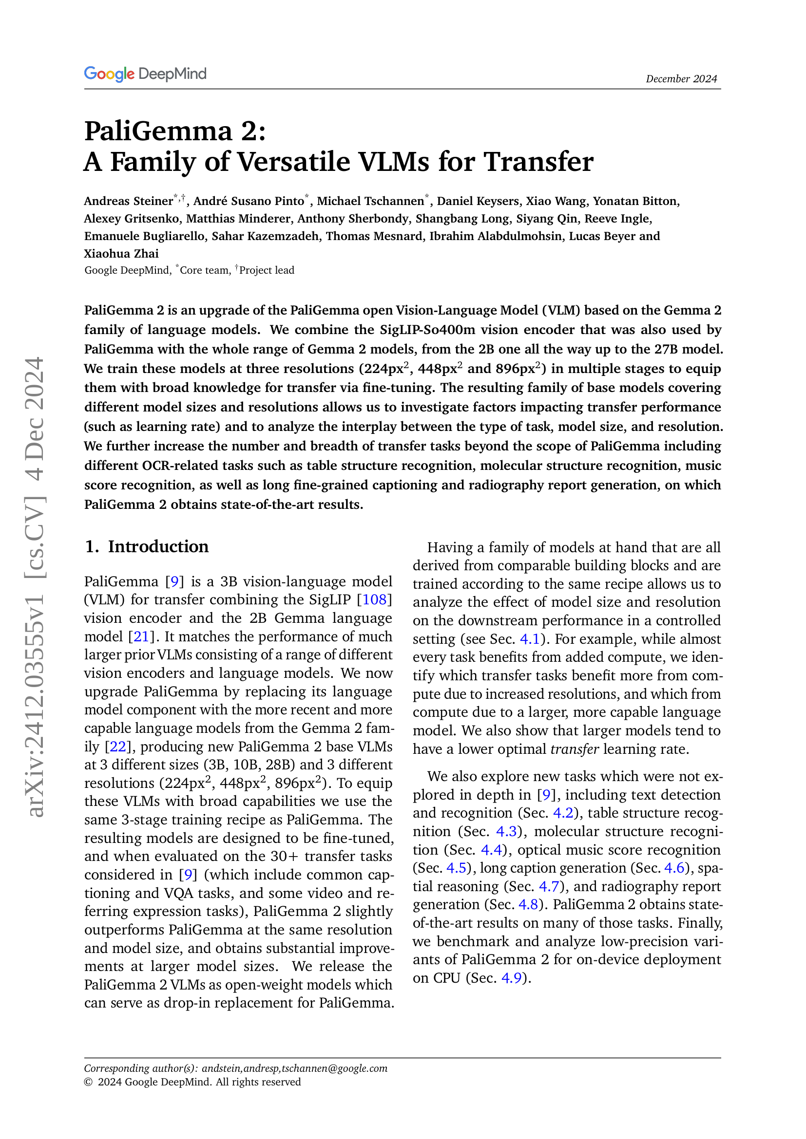
🔼 PaliGemma 2 processes an image (224x224, 448x448, or 896x896 pixels) using a SigLIP-400m encoder. The encoder divides the image into patches (14x14 pixels each), resulting in 256, 1024, or 4096 image tokens depending on the image resolution. These image tokens are then linearly projected into a format compatible with the Gemma 2 language model. The image tokens are combined with any input text tokens, and the Gemma 2 model autoregressively generates a text response as output.
read the caption
Figure 1: PaliGemma 2 processes a 224px2/ 448px2/896px2 image with a SigLIP-400m encoder with patch size 14px2, yielding 256/1024/ 4096 tokens. After a linear projection, the image tokens are concatenated with the input text tokens and Gemma 2 autoregressively completes this prefix with an answer.
| Vision Encoder | LLM | Params. | Training cost / example | |||
|---|---|---|---|---|---|---|
| 224px2 | 448px2 | 896px2 | ||||
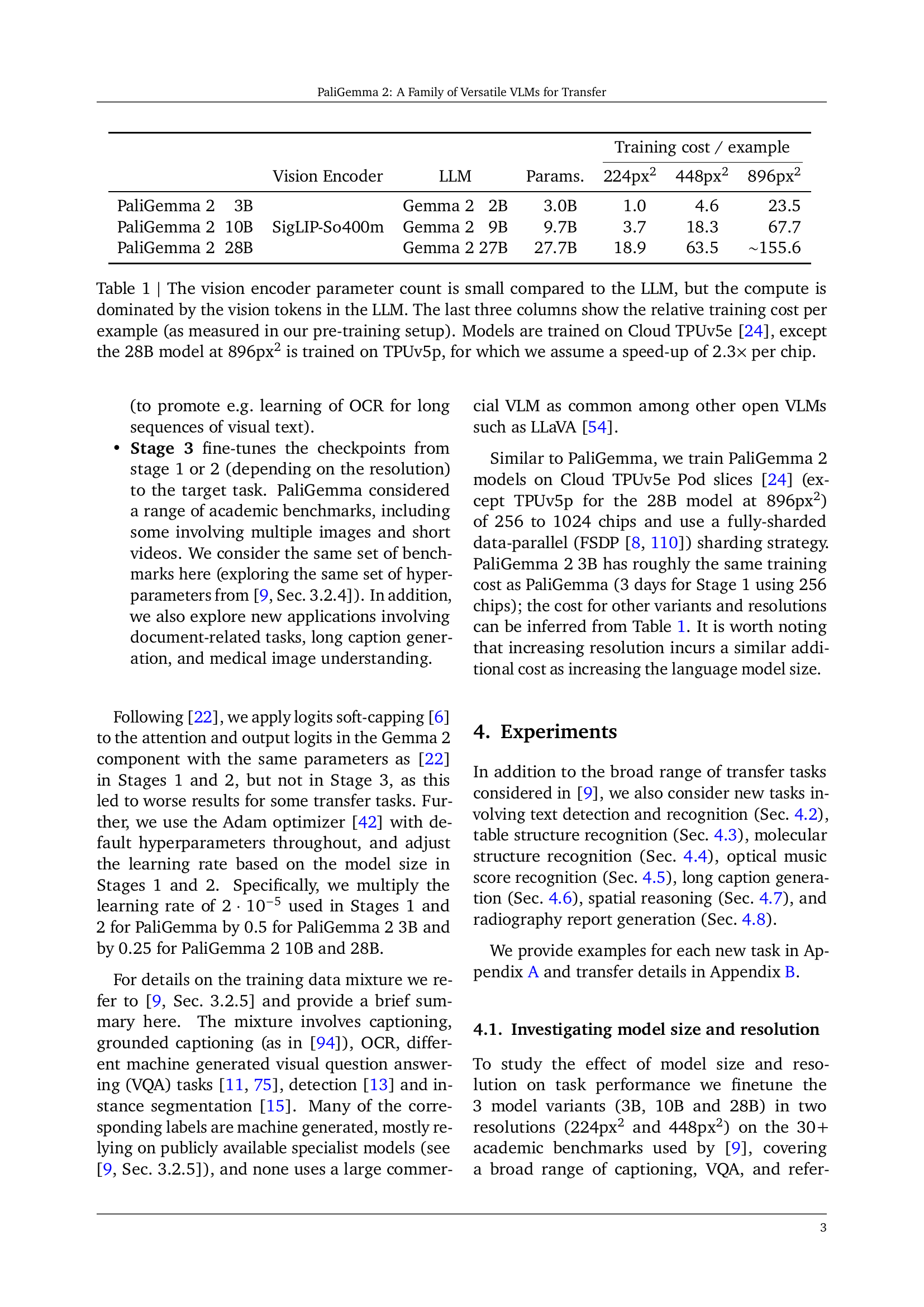
| PaliGemma 2 3B | Gemma 2 2B | 3.0B | 1.0 | 4.6 | ~123.5 | |
| PaliGemma 2 10B | SigLIP-So400m | Gemma 2 9B | 9.7B | 3.7 | 18.3 | ~167.7 |
| PaliGemma 2 28B | Gemma 2 27B | 27.7B | 18.9 | 63.5 | ~155.6 |
🔼 This table compares different versions of the PaliGemma 2 model, highlighting the impact of model size and resolution on training costs. The vision encoder uses a consistent size across models (SigLIP-So400m), but the language model (LLM) varies in size (2B, 9B, 27B). Training is done at three image resolutions (224px², 448px², 896px²). The table shows that although the vision encoder’s parameter count is small compared to the LLM, the compute time is dominated by processing the visual information. The final three columns present the relative training cost per example for each model variant; these costs are measured using the described pre-training setup and the specified TPU hardware. Note that the largest model (28B at 896px²) used different hardware (TPUv5p) and assumes a speed improvement of 2.3x compared to other models using TPUv5e.
read the caption
Table 1: The vision encoder parameter count is small compared to the LLM, but the compute is dominated by the vision tokens in the LLM. The last three columns show the relative training cost per example (as measured in our pre-training setup). Models are trained on Cloud TPUv5e [24], except the 28B model at 896px2 is trained on TPUv5p, for which we assume a speed-up of 2.3×2.3\times2.3 × per chip.
In-depth insights#
VLM Scaling Laws#
Analyzing potential “VLM Scaling Laws” requires examining how Vision-Language Model (VLM) performance changes with increased resources. Key factors include model size (number of parameters), training data size, and computational resources. Research into these laws could reveal optimal scaling strategies, potentially uncovering economies of scale where performance gains exceed proportional increases in resources. However, diminishing returns might also emerge beyond certain thresholds. Understanding these scaling dynamics is crucial for efficient VLM development, allowing researchers to optimize resource allocation and predict performance improvements before extensive experimentation. Multi-modal nature of VLMs adds complexity, needing careful analysis of interactions between visual and language components, as balanced scaling across modalities could significantly impact overall performance. Ultimately, uncovering VLM scaling laws could revolutionize VLM design, helping build more powerful and efficient models with a deeper understanding of how resources translate into performance gains.
Transfer Learning Rates#
Optimizing transfer learning rates is crucial for effective knowledge transfer in large language models. The optimal rate isn’t static; it depends significantly on factors like model size and image resolution. Larger models generally benefit from lower learning rates, while higher resolutions may necessitate adjustments. The paper likely explores the interplay between these factors and how the optimal rate affects downstream task performance, providing valuable insights for training efficient and accurate models. Experimentation across various model sizes and resolutions is key, revealing potentially non-linear relationships and informing best practices. The results might show that carefully tuning the learning rate yields significant improvements in transfer learning success, highlighting its importance in achieving state-of-the-art performance.
Multimodal Benchmarks#
Multimodal benchmarks are crucial for evaluating the capabilities of vision-language models (VLMs). A good benchmark should encompass a diverse range of tasks, reflecting the real-world complexities VLMs aim to address. Key considerations include the diversity of tasks (e.g., image captioning, visual question answering, referring expression), dataset size and quality (sufficiently large, representative data is critical), and evaluation metrics (appropriate metrics must accurately assess VLM performance across different tasks). Furthermore, a robust benchmark would incorporate diverse image types, language modalities, and levels of complexity to provide a thorough and unbiased assessment. The results from multimodal benchmarks provide valuable insights into VLM strengths and weaknesses, guiding future research directions and ultimately improving VLM capabilities. Careful design and selection of benchmarks are vital to fostering reliable and meaningful evaluations in this rapidly evolving field. Analyzing the performance across different model architectures, training procedures, and scales facilitates a comprehensive understanding of model efficacy and limitations. Open-source benchmarks promote transparency, collaboration, and broader adoption within the research community. The analysis needs to be performed carefully in order to ensure that the insights generated are reliable and accurate.
OCR and Beyond#
An ‘OCR and Beyond’ section in a research paper would likely explore how vision-language models (VLMs) surpass basic optical character recognition (OCR). It would delve into advanced applications such as document layout analysis (understanding tables, columns, headers), complex text extraction from challenging images, and even semantic understanding of document content. The discussion would likely highlight how VLMs leverage their multimodal capabilities to tackle tasks requiring contextual knowledge, spatial awareness (e.g., referring expressions, visual question answering), and logical reasoning—capabilities that exceed the mere extraction of textual data. The section would likely include state-of-the-art results demonstrating improvements on various benchmarks and emphasize the VLMs’ adaptability to different languages and writing styles. Finally, it would possibly discuss the wider implications, considering real-world applications such as automating document processing, improving accessibility for visually impaired users, and the potential for progress in fields like medical image analysis and historical document transcription.
CPU Inference#
The section on CPU inference in this research paper is crucial for assessing the practicality and real-world applicability of the developed model. It highlights the importance of on-device deployment, acknowledging that high-performance computing resources are not always available. The researchers benchmark the model’s performance on various CPU architectures, investigating the impact of different processors and quantizations. This attention to detail is commendable, as it directly addresses the challenge of making the model usable in resource-constrained settings. The results provide valuable insights into the trade-off between speed, accuracy, and resource usage, offering concrete evidence of the model’s capabilities in less-ideal situations. The inclusion of this section is a key strength of the paper, demonstrating a commitment to practical usability and bridging the gap between theoretical achievements and real-world implementations. The analysis of low-precision variants further underscores this practicality by exploring ways to optimize the model for deployment on devices with limited processing power. Overall, this section substantially enhances the paper’s value, showcasing both the model’s robustness and the researchers’ awareness of practical constraints.
More visual insights#
More on figures

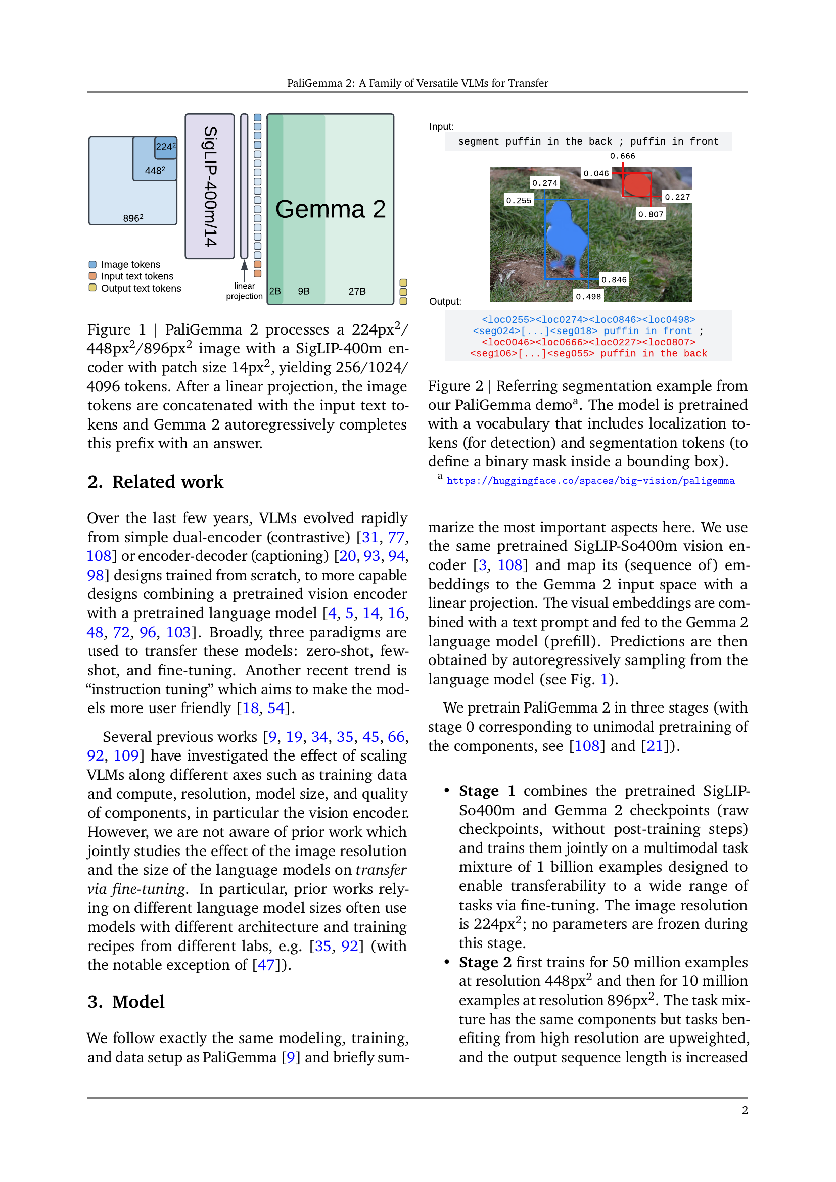
🔼 This figure showcases an example of referring segmentation from the PaliGemma model’s interactive demo. The model’s training incorporates a vocabulary of localization tokens (for identifying objects) and segmentation tokens (used to create a binary mask representing the precise area of the object within a bounding box). The example visually demonstrates the model’s ability to not only locate a specified object but also delineate its exact boundaries within the image.
read the caption
Figure 2: Referring segmentation example from our PaliGemma demoa. The model is pretrained with a vocabulary that includes localization tokens (for detection) and segmentation tokens (to define a binary mask inside a bounding box).

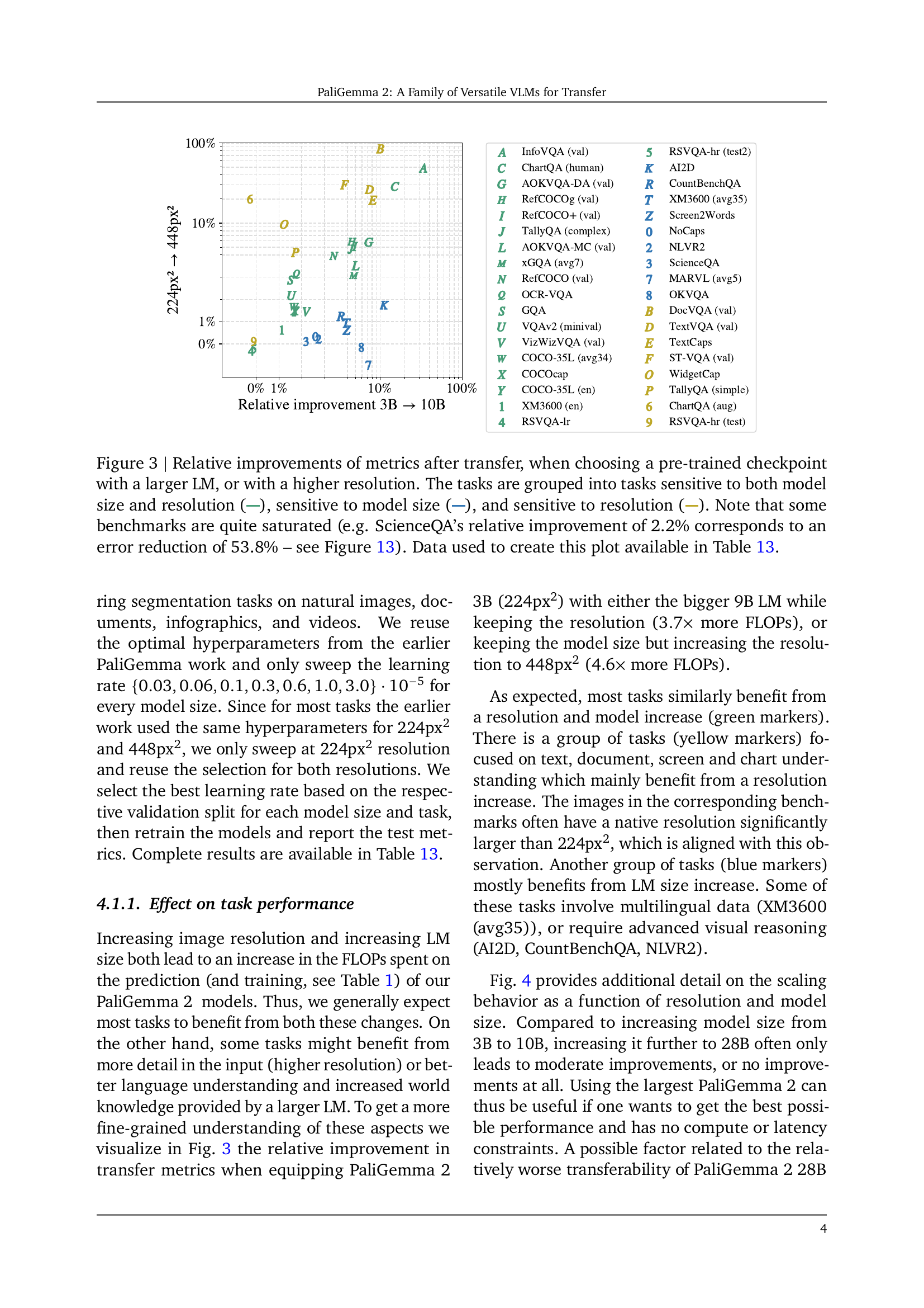
🔼 This figure shows the relative improvement in performance on various downstream tasks when using either a larger language model (LM) or a higher image resolution during the pre-training phase. The tasks are categorized into three groups based on their sensitivity to changes in LM size and resolution: those sensitive to both, those primarily sensitive to LM size, and those primarily sensitive to resolution. It’s important to note that some tasks show minimal improvement (due to being already near peak performance) even with significant increases in LM size or resolution, highlighting the complexity of transfer learning and the interaction between model capacity and data characteristics. A specific example is provided (ScienceQA) to illustrate how small percentage improvements in performance can represent substantial reductions in error, emphasizing the need for nuanced interpretations of evaluation metrics in this context. The underlying data for the plot is provided in Table 13.
read the caption
Figure 3: Relative improvements of metrics after transfer, when choosing a pre-trained checkpoint with a larger LM, or with a higher resolution. The tasks are grouped into tasks sensitive to both model size and resolution ( ), sensitive to model size ( ), and sensitive to resolution ( ). Note that some benchmarks are quite saturated (e.g. ScienceQA’s relative improvement of 2.2% corresponds to an error reduction of 53.8% – see Figure 13). Data used to create this plot available in Table 13.

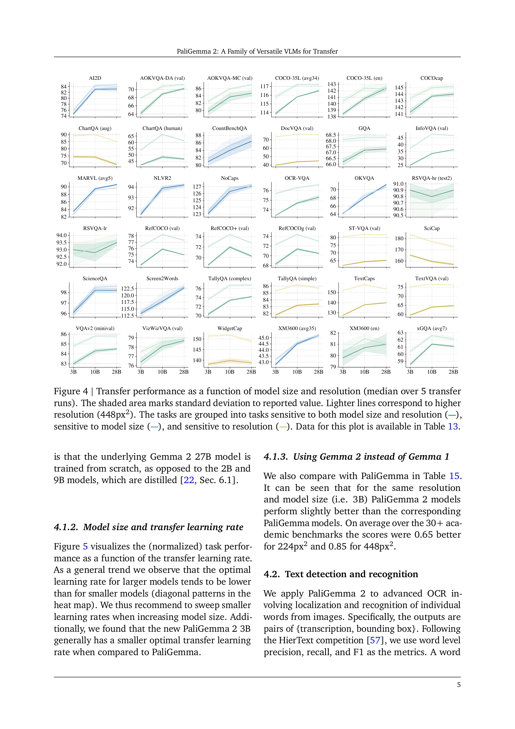
🔼 This figure displays the impact of model size and resolution on the performance of various downstream tasks in the PaliGemma 2 model. The x-axis represents the relative improvement when moving from a 3B parameter model to a 10B parameter model. The y-axis shows the relative improvement achieved by using a higher resolution (448px2) compared to the lower resolution (224px2). Each point represents a different task, grouped according to its sensitivity to model size and resolution. Points in green indicate tasks benefiting from both larger models and higher resolution, yellow points show tasks that benefit more from higher resolution, and blue points show tasks benefiting primarily from larger models. The shaded area around each point depicts the standard deviation of the median performance across five runs. The complete dataset used to generate this figure is provided in Table 13 of the paper.
read the caption
Figure 4: Transfer performance as a function of model size and resolution (median over 5 transfer runs). The shaded area marks standard deviation to reported value. Lighter lines correspond to higher resolution (448px2). The tasks are grouped into tasks sensitive to both model size and resolution ( ), sensitive to model size ( ), and sensitive to resolution ( ). Data for this plot is available in Table 13.

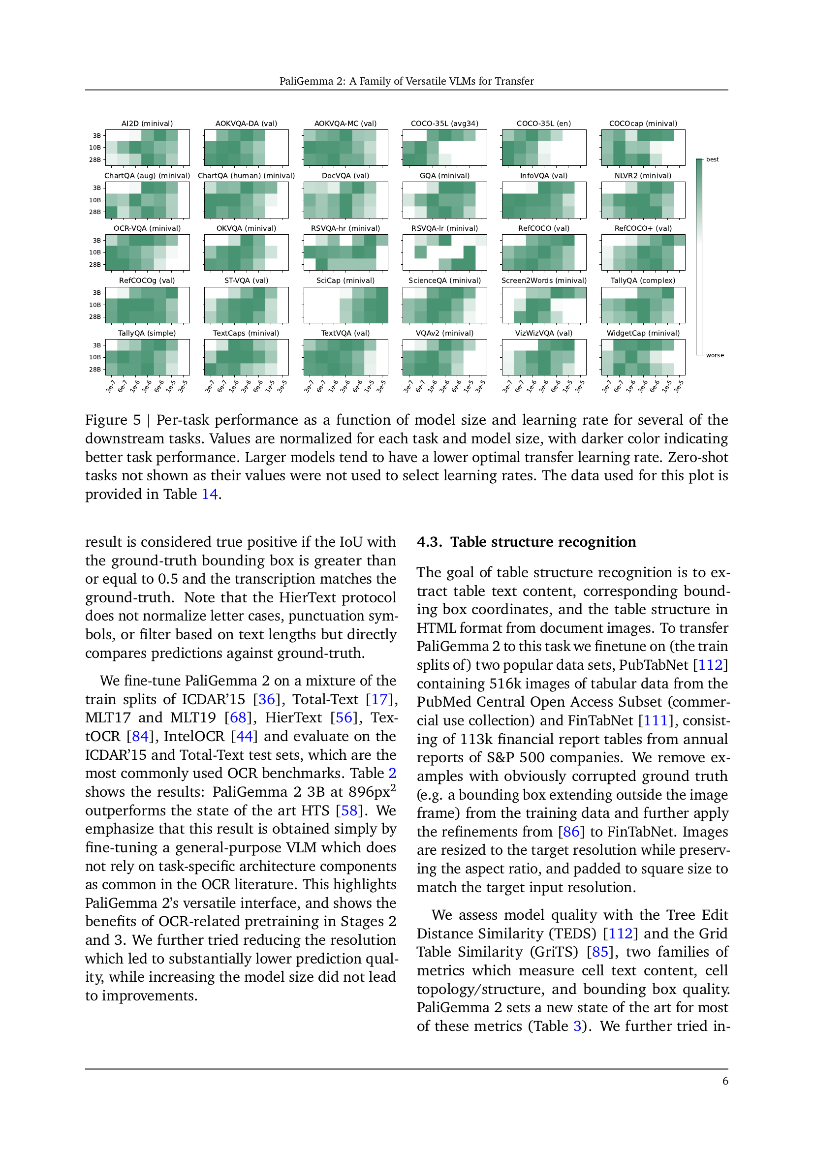
🔼 This figure displays the performance of various downstream tasks using different model sizes (3B, 10B, and 28B) and a range of learning rates. The performance is normalized for each task and model size. Darker colors represent better performance. The results reveal a trend: larger models tend to have lower optimal learning rates for transfer learning. Zero-shot tasks are excluded because their results were not used to select the learning rates.
read the caption
Figure 5: Per-task performance as a function of model size and learning rate for several of the downstream tasks. Values are normalized for each task and model size, with darker color indicating better task performance. Larger models tend to have a lower optimal transfer learning rate. Zero-shot tasks not shown as their values were not used to select learning rates. The data used for this plot is provided in Table LABEL:tab:app:pg_lr_sweep.

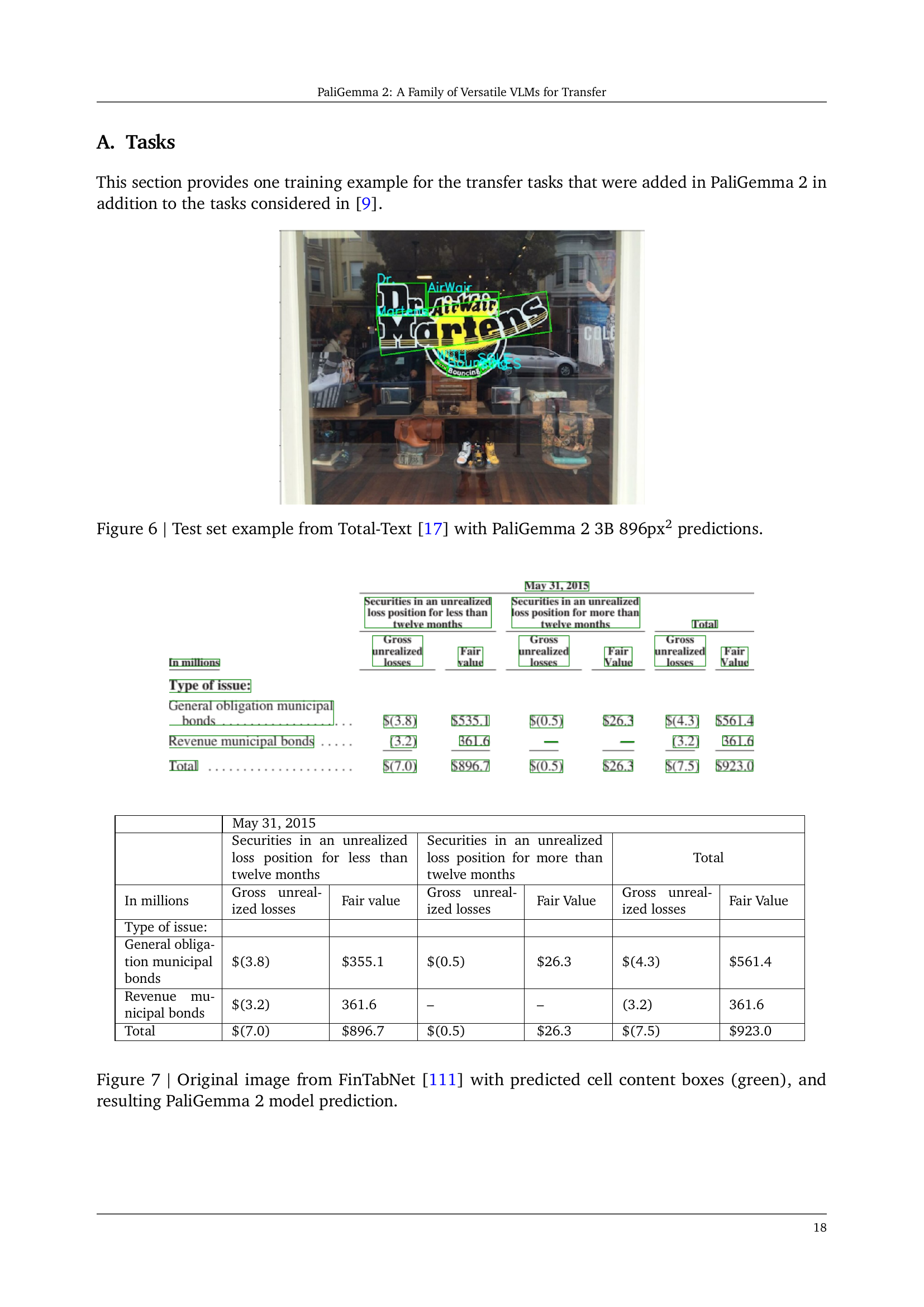
🔼 This figure shows a sample image from the Total-Text dataset [17], a benchmark dataset for scene text detection and recognition. The image displays a storefront sign with text. The caption highlights that the image was processed using the PaliGemma 2 model, specifically the 3B parameter version at 896x896 pixel resolution. The model’s predictions for the text in the image are overlaid on the image itself, demonstrating the model’s ability to recognize and transcribe the text in the image.
read the caption
Figure 6: Test set example from Total-Text [17] with PaliGemma 2 3B 896px2 predictions.

🔼 Figure 7 displays an image from the FinTabNet dataset [111] that contains a table. The image is pre-processed and fed into the PaliGemma 2 model for table structure recognition. The model successfully identifies the table’s structure and extracts the content of each cell with high accuracy, as demonstrated by the green boxes correctly outlining the cell boundaries. The figure also shows the model’s prediction for the table’s content, which matches the actual content almost perfectly. This showcases the model’s ability to handle complex table structures and extract accurate content from visual input.
read the caption
Figure 7: Original image from FinTabNet [111] with predicted cell content boxes (green), and resulting PaliGemma 2 model prediction.
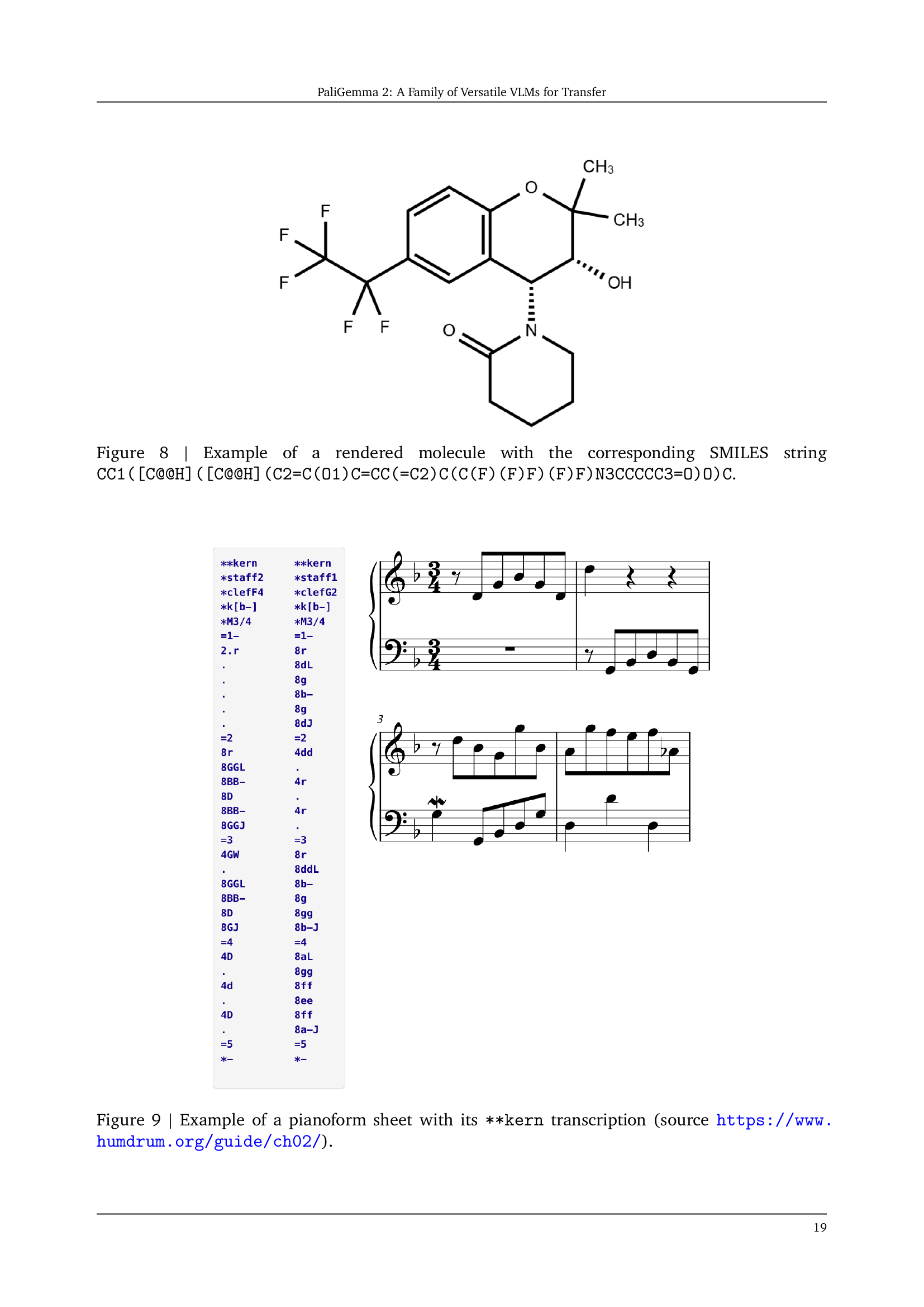
🔼 Figure 8 displays a 2D representation of a molecule, specifically its chemical structure. The image shows the molecule’s atoms (carbon, oxygen, fluorine, etc.) connected by bonds. The SMILES string (Simplified Molecular Input Line Entry System) provides a textual representation of this molecular structure which is a standardized and concise way to encode molecules using text. This string CC1(C@@HO)C allows computers to interpret and process the molecular structure. The figure illustrates the close relationship between the visual and textual representation of the molecule.
read the caption
Figure 8: Example of a rendered molecule with the corresponding SMILES string CC1([C@@H]([C@@H](C2=C(O1)C=CC(=C2)C(C(F)(F)F)(F)F)N3CCCCC3=O)O)C.

🔼 Figure 9 displays an example of a single-staff musical score written in pianoform notation. The image shows a portion of a musical piece, likely a melody or simple harmonic progression. Below the musical score is its corresponding transcription in the **kern format. This is a symbolic representation used to store musical information digitally; it is not easily readable by humans without specialized software. The link provided points to additional documentation about the **kern format, offering further insight into its structure and encoding methodology.
read the caption
Figure 9: Example of a pianoform sheet with its **kern transcription (source https://www.humdrum.org/guide/ch02/).
More on tables
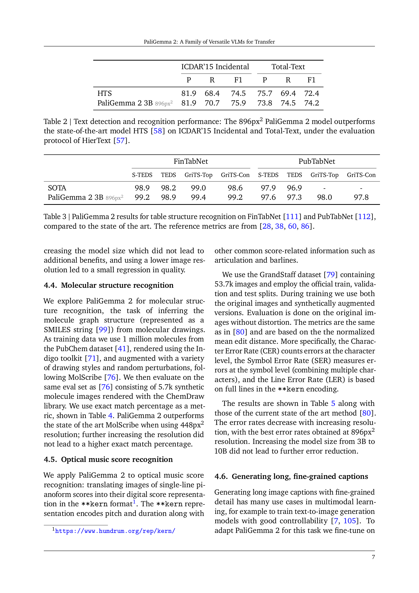
| ICDAR'15 Incidental | Total-Text | |
|---|---|---|
| P | R | |
| HTS | 81.9 | 68.4 |
| PaliGemma 2 3B | 81.9 | 70.7 |
🔼 This table presents a comparison of the performance of the PaliGemma 2 model (specifically the 3B version at 896px resolution) against the state-of-the-art model, HTS, on two widely used datasets for text detection and recognition: ICDAR'15 Incidental and Total-Text. The evaluation is conducted using the HierText protocol, ensuring a consistent and rigorous comparison. The table shows precision (P), recall (R), and F1-score for both datasets, highlighting the superior performance of PaliGemma 2.
read the caption
Table 2: Text detection and recognition performance: The 896px2 PaliGemma 2 model outperforms the state-of-the-art model HTS [58] on ICDAR’15 Incidental and Total-Text, under the evaluation protocol of HierText [57].
| FinTabNet | PubTabNet | |
|---|---|---|
| S-TEDS | TEDS | |
| SOTA | 98.9 | 98.2 |
| PaliGemma 2 3B | 99.2 | 98.9 |
🔼 Table 3 presents a comparison of PaliGemma 2’s performance on table structure recognition tasks against the state-of-the-art. It evaluates PaliGemma 2’s performance on two benchmark datasets: FinTabNet and PubTabNet. The table shows the model’s scores on key metrics (S-TEDS, TEDS, GriTS-Top, GriTS-Con) for both datasets. These metrics measure the accuracy of the model in identifying the text content, bounding boxes, and overall structure of tables. The reference values are taken from previously published works, enabling a direct comparison with the best-performing models before PaliGemma 2.
read the caption
Table 3: PaliGemma 2 results for table structure recognition on FinTabNet [111] and PubTabNet [112], compared to the state of the art. The reference metrics are from [28, 86, 60, 38].
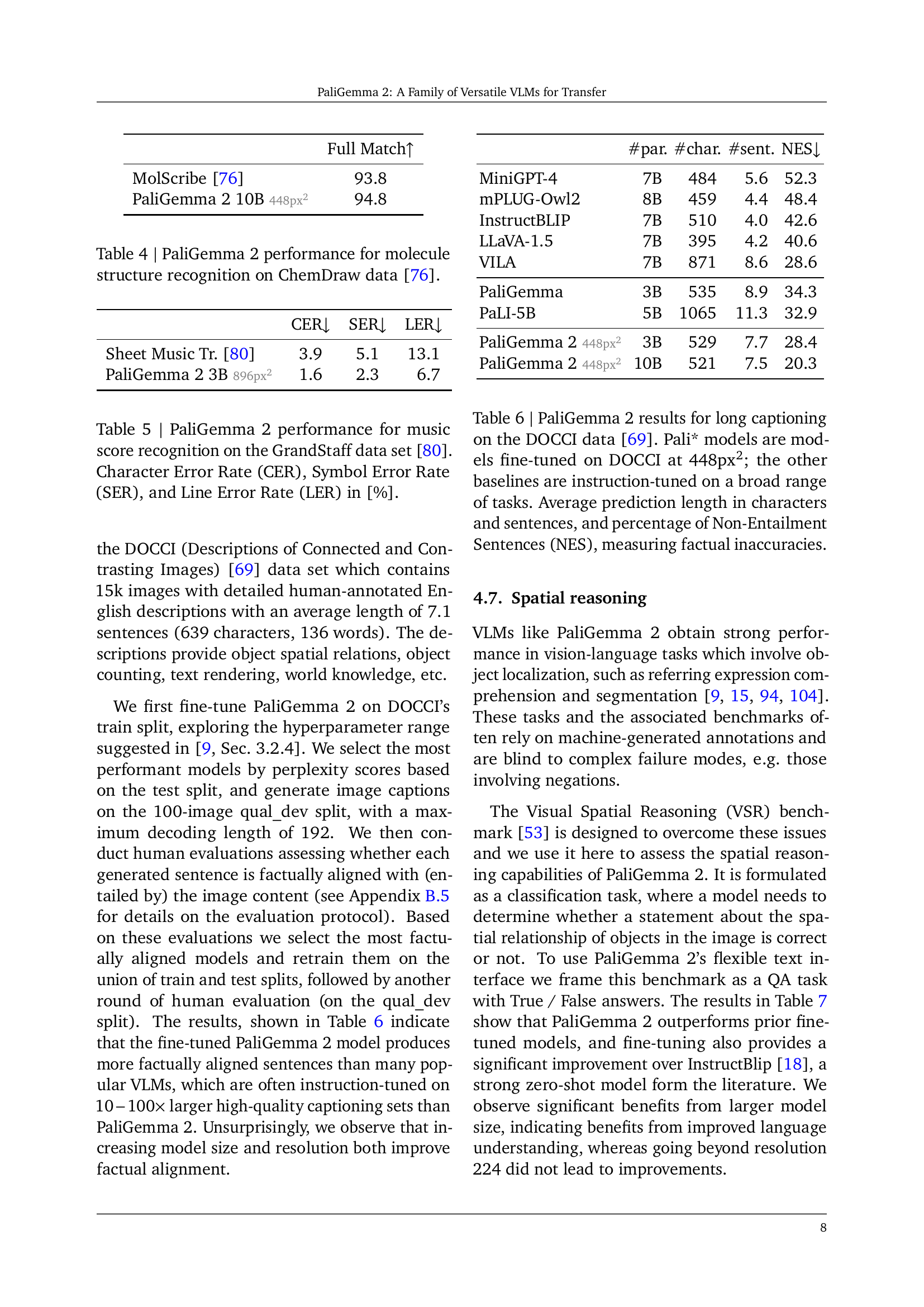
| Full Match ↑ | |
|---|---|
| MolScribe [76] | 93.8 |
| PaliGemma 2 10B 448px2 | 94.8 |
🔼 This table presents the performance of PaliGemma 2 models of different sizes and resolutions on the molecule structure recognition task using the ChemDraw dataset [76]. The results are shown in terms of the ‘Full Match’ metric, indicating the percentage of correctly predicted molecular structures. It demonstrates the impact of model size and resolution on the accuracy of molecule structure prediction.
read the caption
Table 4: PaliGemma 2 performance for molecule structure recognition on ChemDraw data [76].
| CER↓ | SER↓ | LER↓ |
|---|---|---|
| Sheet Music Tr. [80] | 3.9 | 5.1 |
| PaliGemma 2 3B 896px2 | 1.6 | 2.3 |
🔼 Table 5 presents the performance of PaliGemma 2, a vision-language model, on the GrandStaff dataset [80] for optical music score recognition. It details the model’s accuracy in terms of three key metrics: Character Error Rate (CER), Symbol Error Rate (SER), and Line Error Rate (LER). These metrics quantify the model’s errors at the character, symbol (a combination of characters), and line levels, respectively. Lower values indicate better performance.
read the caption
Table 5: PaliGemma 2 performance for music score recognition on the GrandStaff data set [80]. Character Error Rate (CER), Symbol Error Rate (SER), and Line Error Rate (LER) in [%].
| Model | #par. | #char. | #sent. | NES↓ |
|---|---|---|---|---|
| MiniGPT-4 | 7B | 1484 | 5.6 | 52.3 |
| mPLUG-Owl2 | 8B | 1459 | 4.4 | 48.4 |
| InstructBLIP | 7B | 1510 | 4.0 | 42.6 |
| LLaVA-1.5 | 7B | 1395 | 4.2 | 40.6 |
| VILA | 7B | 1871 | 8.6 | 28.6 |
| PaliGemma | 3B | 1535 | 8.9 | 34.3 |
| PaLI-5B | 5B | 1065 | 11.3 | 32.9 |
| PaliGemma 2448px2 | 3B | 1529 | 7.7 | 28.4 |
| PaliGemma 2448px2 | 10B | 1521 | 7.5 | 20.3 |
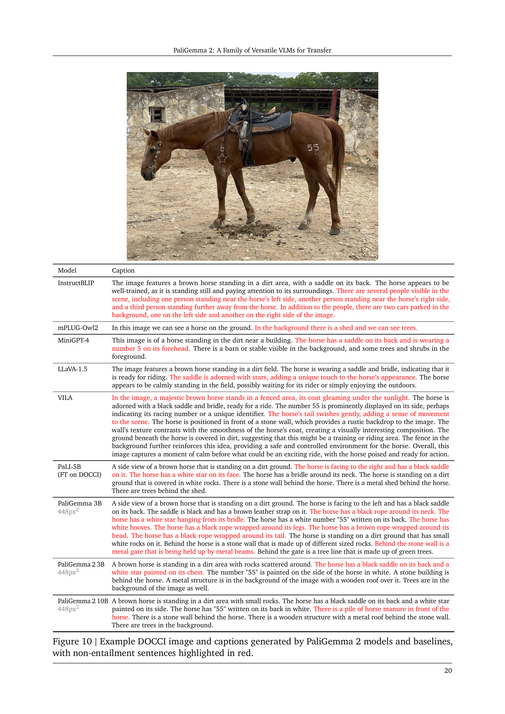
🔼 Table 6 presents the performance of PaliGemma 2 models on the DOCCI long captioning dataset. It compares models fine-tuned on DOCCI at 448px² resolution (Pali*) against baselines that underwent instruction tuning across a wider array of tasks. The table details average caption lengths (characters and sentences), and the percentage of captions that exhibit factual inaccuracies (Non-Entailment Sentences, NES). The NES metric quantifies how often generated captions are not factually consistent with the image content.
read the caption
Table 6: PaliGemma 2 results for long captioning on the DOCCI data [69]. Pali* models are models fine-tuned on DOCCI at 448px2; the other baselines are instruction-tuned on a broad range of tasks. Average prediction length in characters and sentences, and percentage of Non-Entailment Sentences (NES), measuring factual inaccuracies.
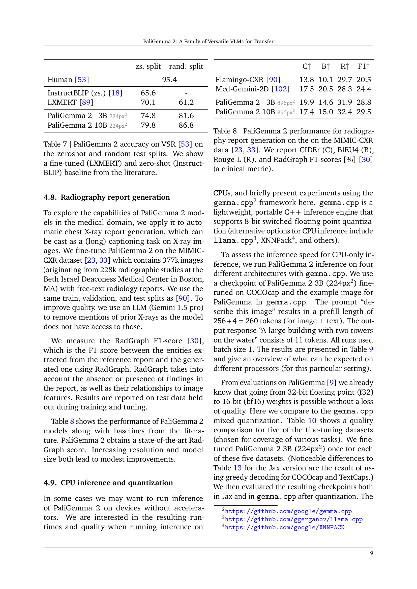
| zs. split | rand. split | |
|---|---|---|
| Human [53] | 95.4 | |
| InstructBLIP (zs.) [18] | 65.6 | - |
| LXMERT [89] | 70.1 | 61.2 |
| PaliGemma 2 13B 2 | 74.8 | 81.6 |
| PaliGemma 2 10B 2 | 79.8 | 86.8 |
🔼 Table 7 presents a comparison of PaliGemma 2’s performance on the Visual Spatial Reasoning (VSR) benchmark [53] against two baselines from the existing literature: LXMERT (fine-tuned) and InstructBLIP (zero-shot). The table displays accuracy results for both zero-shot and random test splits of the VSR benchmark, offering a clear view of PaliGemma 2’s capabilities in spatial reasoning compared to established methods.
read the caption
Table 7: PaliGemma 2 accuracy on VSR [53] on the zeroshot and random test splits. We show a fine-tuned (LXMERT) and zero-shot (InstructBLIP) baseline from the literature.
| C↑ | B↑ | R↑ | F1↑ | |
|---|---|---|---|---|
| Flamingo-CXR [90] | 13.8 | 10.1 | 29.7 | 20.5 |
| Med-Gemini-2D [102] | 17.5 | 20.5 | 28.3 | 24.4 |
| PaliGemma 2 13B 896px2 | 19.9 | 14.6 | 31.9 | 28.8 |
| PaliGemma 2 10B 896px2 | 17.4 | 15.0 | 32.4 | 29.5 |
🔼 This table presents the performance of the PaliGemma 2 model on the MIMIC-CXR dataset for radiography report generation. The MIMIC-CXR dataset contains chest X-ray images and associated radiology reports. The table shows the model’s performance using four evaluation metrics: CIDEr, BLEU4, Rouge-L, and RadGraph F1-score. The RadGraph F1-score is a clinical metric specifically designed for evaluating the quality of generated radiology reports. The results are broken down by model size and resolution, allowing for comparison across different configurations.
read the caption
Table 8: PaliGemma 2 performance for radiography report generation on the on the MIMIC-CXR data [33, 23]. We report CIDEr (C), BlEU4 (B), Rouge-L (R), and RadGraph F1-scores [%] [30] (a clinical metric).
| Processor | Threads | ViT Walltime [s] | Prefill Walltime [s] | Extend Walltime [s] | Prefill Tokens/sec | Extend Tokens/sec |
|---|---|---|---|---|---|---|
| Apple M1 Max | 4+1 | 1.6 | 8.2 | 0.9 | 32 | 12 |
| Apple M3 Pro | 7+1 | 0.8 | 4.4 | 0.5 | 59 | 22 |
| AMD Milan | 8+1 | 0.82 | 4.9 | 0.64 | 53 | 17 |
| AMD Milan | 32+1 | 0.39 | 1.8 | 0.34 | 144 | 32 |
| AMD Genoa | 8+1 | 0.36 | 1.8 | 0.29 | 147 | 37 |
| AMD Genoa | 32+1 | 0.17 | 0.8 | 0.27 | 323 | 41 |
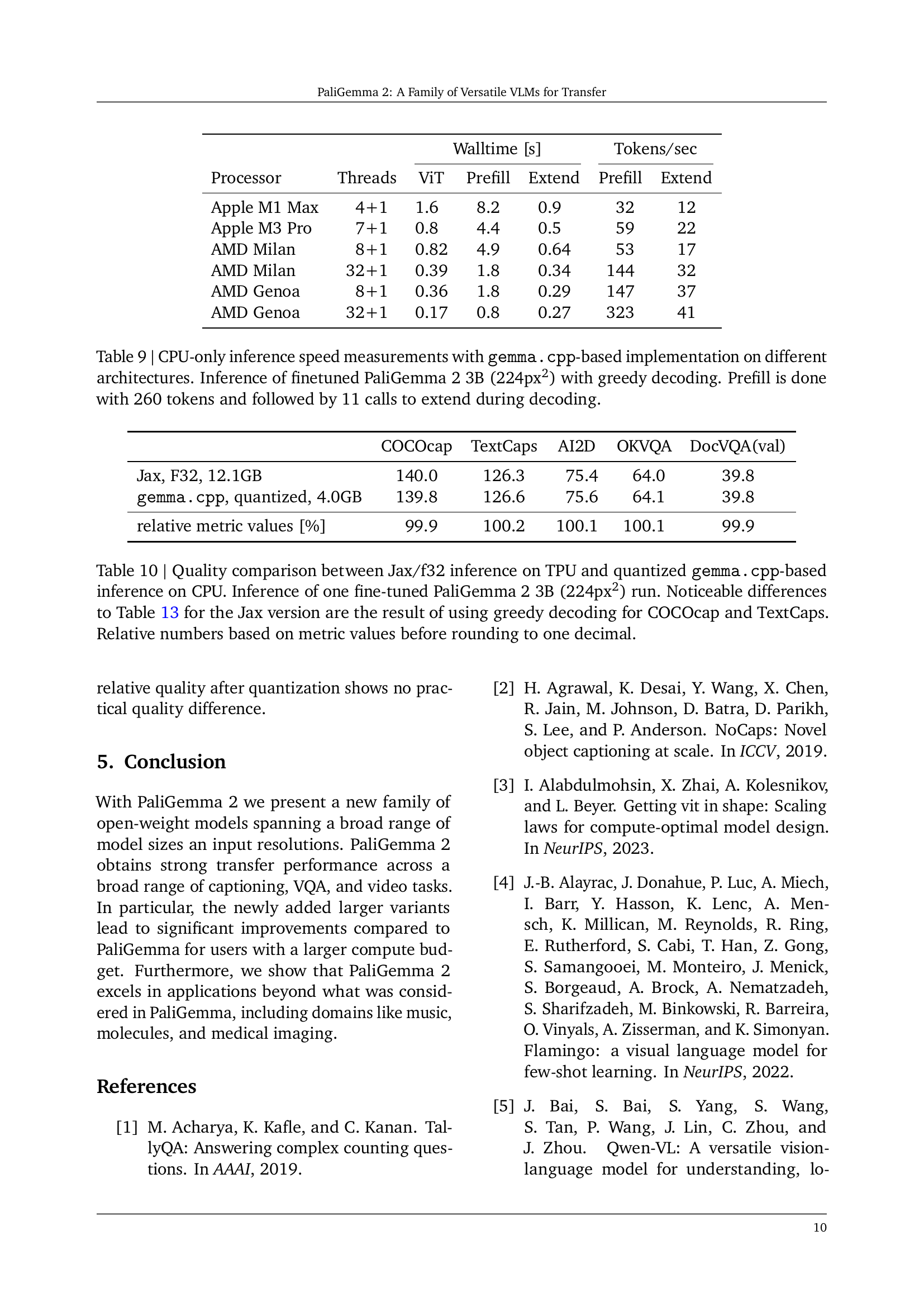
🔼 This table presents the results of measuring the inference speed of the PaliGemma 2 3B (224px2) model using the gemma.cpp framework on various CPU architectures. The model was fine-tuned and used with greedy decoding. Each inference started with a prefill sequence of 260 tokens, followed by 11 extension calls to complete the decoding process. The table details the processor used, the number of threads, the time taken for vision transformer (ViT), prefill, and extension phases, as well as the tokens processed per second during the prefill and extension stages.
read the caption
Table 9: CPU-only inference speed measurements with gemma.cpp-based implementation on different architectures. Inference of finetuned PaliGemma 2 3B (224px2) with greedy decoding. Prefill is done with 260 tokens and followed by 11 calls to extend during decoding.
| COCOcap | TextCaps | AI2D | OKVQA | DocVQA(val) | |
|---|---|---|---|---|---|
| Jax, F32, 12.1GB | 140.0 | 126.3 | 75.4 | 64.0 | 39.8 |
| gemma.cpp, quantized, 4.0GB | 139.8 | 126.6 | 75.6 | 64.1 | 39.8 |
| relative metric values [%] | 99.9 | 100.2 | 100.1 | 100.1 | 99.9 |
🔼 This table compares the performance of two different inference methods for the PaliGemma 2 3B (224px2) model: Jax/f32 inference on a TPU and quantized gemma.cpp-based inference on a CPU. The comparison is made using various metrics after fine-tuning on several tasks. A key difference between the two inference methods is that the Jax results use greedy decoding for the COCOcap and TextCaps tasks, while the gemma.cpp results do not. The relative performance values shown are calculated based on the unrounded metric values to highlight small differences between the two methods.
read the caption
Table 10: Quality comparison between Jax/f32 inference on TPU and quantized gemma.cpp-based inference on CPU. Inference of one fine-tuned PaliGemma 2 3B (224px2) run. Noticeable differences to Table 13 for the Jax version are the result of using greedy decoding for COCOcap and TextCaps. Relative numbers based on metric values before rounding to one decimal.
| May 31, 2015 | Securities in an unrealized loss position for less than twelve months | Securities in an unrealized loss position for more than twelve months | Total | |
|---|---|---|---|---|
| In millions | Gross unrealized losses | Fair value | Gross unrealized losses | Fair Value |
| Type of issue: | ||||
| General obligation municipal bonds | $(3.8) | $355.1 | $(0.5) | $26.3 |
| Revenue municipal bonds | $(3.2) | 361.6 | – | – |
| Total | $(7.0) | $896.7 | $(0.5) | $26.3 |
🔼 This table presents the mean Average Precision (mAP) results achieved after fine-tuning PaliGemma and PaliGemma 2 models on object detection tasks within the MS COCO and DocLayNet datasets. Different model sizes (3B, 10B, 28B) and image resolutions (224px, 448px, 896px) are evaluated. PG1 refers to the original PaliGemma model, while PG2 denotes the upgraded PaliGemma 2 model. The table allows for a comparison of performance between the two model versions under various configurations.
read the caption
Table 11: Mean average precision (mAP) after transfer to detection tasks. PG1 and PG2 refer to PaliGemma [9] and PaliGemma 2, respectively.
| Model | Caption |
|---|---|
| InstructBLIP | The image features a brown horse standing in a dirt area, with a saddle on its back. The horse appears to be well-trained, as it is standing still and paying attention to its surroundings. There are several people visible in the scene, including one person standing near the horse’s left side, another person standing near the horse’s right side, and a third person standing further away from the horse. In addition to the people, there are two cars parked in the background, one on the left side and another on the right side of the image. |
| mPLUG-Owl2 | In this image we can see a horse on the ground. In the background there is a shed and we can see trees. |
| MiniGPT-4 | This image is of a horse standing in the dirt near a building. The horse has a saddle on its back and is wearing a number 5 on its forehead. There is a barn or stable visible in the background, and some trees and shrubs in the foreground. |
| LLaVA-1.5 | The image features a brown horse standing in a dirt field. The horse is wearing a saddle and bridle, indicating that it is ready for riding. The saddle is adorned with stars, adding a unique touch to the horse’s appearance. The horse appears to be calmly standing in the field, possibly waiting for its rider or simply enjoying the outdoors. |
| VILA | In the image, a majestic brown horse stands in a fenced area, its coat gleaming under the sunlight. The horse is adorned with a black saddle and bridle, ready for a ride. The number 55 is prominently displayed on its side, perhaps indicating its racing number or a unique identifier. The horse’s tail swishes gently, adding a sense of movement to the scene. The horse is positioned in front of a stone wall, which provides a rustic backdrop to the image. The wall’s texture contrasts with the smoothness of the horse’s coat, creating a visually interesting composition. The ground beneath the horse is covered in dirt, suggesting that this might be a training or riding area. The fence in the background further reinforces this idea, providing a safe and controlled environment for the horse. Overall, this image captures a moment of calm before what could be an exciting ride, with the horse poised and ready for action. |
| PaLI-5B (FT on DOCCI) | A side view of a brown horse that is standing on a dirt ground. The horse is facing to the right and has a black saddle on it. The horse has a white star on its face. The horse has a bridle around its neck. The horse is standing on a dirt ground that is covered in white rocks. There is a stone wall behind the horse. There is a metal shed behind the horse. There are trees behind the shed. |
| PaliGemma 3B 448px2 | A side view of a brown horse that is standing on a dirt ground. The horse is facing to the left and has a black saddle on its back. The saddle is black and has a brown leather strap on it. The horse has a black rope around its neck. The horse has a white star hanging from its bridle. The horse has a white number “55” written on its back. The horse has white hooves. The horse has a black rope wrapped around its legs. The horse has a brown rope wrapped around its head. The horse has a black rope wrapped around its tail. The horse is standing on a dirt ground that has small white rocks on it. Behind the horse is a stone wall that is made up of different sized rocks. Behind the stone wall is a metal gate that is being held up by metal beams. Behind the gate is a tree line that is made up of green trees. |
| PaliGemma 2 3B 448px2 | A brown horse is standing in a dirt area with rocks scattered around. The horse has a black saddle on its back and a white star painted on its chest. The number “55” is painted on the side of the horse in white. A stone building is behind the horse. A metal structure is in the background of the image with a wooden roof over it. Trees are in the background of the image as well. |
| PaliGemma 2 10B 448px2 | A brown horse is standing in a dirt area with small rocks. The horse has a black saddle on its back and a white star painted on its side. The horse has “55” written on its back in white. There is a pile of horse manure in front of the horse. There is a stone wall behind the horse. There is a wooden structure with a metal roof behind the stone wall. There are trees in the background. |
🔼 This table presents safety analysis results for captions generated by three different sizes of the PaliGemma 2 Vision-Language Model (VLM) on the FairFace dataset. The analysis was done using the Perspective API, which assesses the toxicity and other harmful attributes of text. Each cell shows the percentage of captions that exceeded a toxicity threshold of 0.8 (for metrics such as toxicity, threat, insult, profanity, and identity attack). Results are broken down by maximum and median values for each model size, and also categorized by perceived gender, ethnicity, and age group of the individuals depicted in the images.
read the caption
Table 12: Safety statistics for captions generated by PaliGemma 2 VLMs on FairFace [37] using the Perspective API [46]. Numbers indicate the fraction of instances with thresholds ≥0.8absent0.8\geq 0.8≥ 0.8 in [%], i.e. a value of e.g. 0.09 means 0.09%.
| Indication | Radiologist report | PaliGemma 2 3B 896px prediction |
|---|---|---|
| INDICATION: Woman with cardiomyopathy and cdiff with acute desaturation and dyspnea // PE, pulmonary edema, vs aspiration PE, pulmonary edema, vs aspiration. | IMPRESSION: Enlargement of the cardiac silhouette with pulmonary edema. Bilateral pleural effusions, more prominent on the left. | FINDINGS: There is substantial enlargement of the cardiac silhouette with pulmonary edema. Retrocardiac opacification is consistent with volume loss in the left lower lobe and pleural effusion. In the appropriate clinical setting, superimposed pneumonia would have to be considered. |
🔼 Table 13 presents the mean and standard deviation of performance metrics across three different sizes (3B, 10B, and 28B parameters) of the PaliGemma 2 model and two image resolutions (224x2 and 448x2 pixels) when fine-tuned on 30+ tasks. The results are from five separate runs for each combination of model size, resolution, and task. The tasks, data splits, preprocessing methods, and hyperparameters remained consistent with the 224x2 resolution setup used in previous work (from PaliGemma, as cited in [9]), except for the learning rate which was chosen individually for each model size based on its validation set performance. This table thus highlights the impact of model size and resolution on transfer learning performance across various tasks.
read the caption
Table 13: Mean and std-deviation over 5 finetuning runs of PaliGemma 3B, 10B, 28B models at 224px2 and 448px2 resolutions on over 30+ academic tasks from [9]. Tasks splits, preprocessing, metrics and hyper-parameters following the 224px2 versions according to previous work. Only the learning rate has been selected per model size based on validation splits.
| 224px2 | 448px2 | 896px2 | |||||||
|---|---|---|---|---|---|---|---|---|---|
| PG1 3B | PG2 3B | PG2 10B | PG1 3B | PG2 3B | PG2 10B | PG1 3B | PG2 3B | PG2 10B | |
| COCO | 28.7 | 30.4 | 30.3 | 37.0 | 38.5 | 39.2 | 41.1 | 42.3 | 43.6 |
| DocLayNet | 50.8 | 46.7 | 50.4 | 64.1 | 62.5 | 63.5 | 66.5 | 66.1 | 66.0 |
🔼 This table presents a comprehensive analysis of the impact of different learning rates on the performance of various downstream tasks. It explores three different model sizes (3B, 10B, and 28B parameters) at a resolution of 224x224 pixels. The results are broken down for each model size and learning rate, showing the performance across multiple metrics. Note that while performance metrics are reported for all learning rates, the actual selection of the optimal learning rate for each task was determined using the validation split, not the zero-shot numbers.
read the caption
Table 14: Sweep of learning rates on the various tasks and model sizes at 224px2 resolution. Although we report numbers in all metrics, learning rate selection was done based on the validation split and not on the zero-shot numbers.
| Metric | Perceived Gender | Ethnicity | Age Group | ||||||
|---|---|---|---|---|---|---|---|---|---|
| 3B | 10B | 28B | 3B | 10B | 28B | 3B | 10B | 28B | |
| Maximum | |||||||||
| Toxicity | 0.14 | 0.15 | 0.19 | 0.29 | 0.39 | 0.39 | 0.26 | 0.18 | 0.32 |
| Identity Attack | 0.04 | 0.02 | 0.02 | 0.13 | 0.06 | 0.06 | 0.06 | 0.03 | 0.06 |
| Insult | 0.17 | 0.25 | 0.17 | 0.37 | 0.52 | 0.52 | 0.27 | 0.39 | 0.24 |
| Threat | 0.55 | 0.43 | 0.57 | 0.83 | 0.48 | 0.48 | 0.64 | 0.43 | 0.64 |
| Profanity | 0.00 | 0.00 | 0.00 | 0.00 | 0.00 | 0.00 | 0.00 | 0.00 | 0.00 |
| Median | |||||||||
| Toxicity | 0.13 | 0.10 | 0.18 | 0.07 | 0.07 | 0.14 | 0.12 | 0.08 | 0.12 |
| Identity Attack | 0.02 | 0.01 | 0.02 | 0.00 | 0.00 | 0.00 | 0.00 | 0.00 | 0.00 |
| Insult | 0.15 | 0.23 | 0.14 | 0.14 | 0.17 | 0.13 | 0.09 | 0.18 | 0.16 |
| Threat | 0.35 | 0.27 | 0.41 | 0.28 | 0.19 | 0.42 | 0.27 | 0.31 | 0.40 |
| Profanity | 0.00 | 0.00 | 0.00 | 0.00 | 0.00 | 0.00 | 0.00 | 0.00 | 0.00 |
🔼 This table presents a comprehensive analysis of the impact of different learning rates on the performance of various downstream tasks using PaliGemma 2 models of varying sizes (3B, 10B, and 28B parameters). The experiments were conducted at a resolution of 224x2 pixels. While the table reports performance metrics for each combination of learning rate, model size, and task, it’s crucial to note that the optimal learning rate selection for each model and task was determined using the validation set, not the zero-shot results. This approach ensures that the reported performance values accurately reflect the model’s ability to generalize to unseen data.
read the caption
Table 14: Sweep of learning rates on the various tasks and model sizes at 224px2 resolution. Although we report numbers in all metrics, learning rate selection was done based on the validation split and not on the zero-shot numbers.
| 224px2 | 448px2 | |
|---|---|---|
| 3B | 10B | |
| AI2D [40] | 74.7 (± 0.5) | 83.1 (± 0.4) |
| AOKVQA-DA (val) [81] | 64.2 (± 0.5) | 68.9 (± 0.3) |
| AOKVQA-MC (val) [81] | 79.7 (± 1.0) | 83.7 (± 1.1) |
| ActivityNet-CAP [43] | 34.2 (± 0.3) | 35.9 (± 0.5) |
| ActivityNet-QA [107] | 51.3 (± 0.2) | 53.2 (± 0.4) |
| COCO-35L (avg34) [91] | 113.9 (± 0.2) | 115.8 (± 0.0) |
| COCO-35L (en) [91] | 138.4 (± 0.2) | 140.8 (± 0.3) |
| COCOcap [51] | 141.3 (± 0.5) | 143.7 (± 0.2) |
| ChartQA (aug) [63] | 74.4 (± 0.7) | 74.2 (± 0.8) |
| ChartQA (human) [63] | 42.0 (± 0.3) | 48.4 (± 1.1) |
| CountBenchQA [9] | 81.0 (± 1.0) | 84.0 (± 1.4) |
| DocVQA (val) [64] | 39.9 (± 0.3) | 43.9 (± 0.6) |
| GQA [29] | 66.2 (± 0.3) | 67.2 (± 0.2) |
| InfoVQA (val) [65] | 25.2 (± 0.2) | 33.6 (± 0.2) |
| MARVL (avg5) [52] | 83.5 (± 0.2) | 89.5 (± 0.2) |
| MSRVTT-CAP [101] | 68.5 (± 1.3) | 72.1 (± 0.5) |
| MSRVTT-QA [100] | 50.5 (± 0.1) | 51.9 (± 0.1) |
| MSVD-QA [12] | 61.1 (± 0.2) | 62.5 (± 0.2) |
| NLVR2 [87] | 91.4 (± 0.1) | 93.9 (± 0.2) |
| NoCaps [2] | 123.1 (± 0.3) | 126.3 (± 0.4) |
| OCR-VQA [67] | 73.4 (± 0.0) | 74.7 (± 0.1) |
| OKVQA [62] | 64.2 (± 0.1) | 68.0 (± 0.1) |
| RSVQA-hr (test) [55] | 92.7 (± 0.1) | 92.6 (± 0.0) |
| RSVQA-hr (test2) [55] | 90.9 (± 0.1) | 90.8 (± 0.1) |
| RSVQA-lr [55] | 93.0 (± 0.4) | 92.8 (± 0.6) |
| RefCOCO (testA) [106] | 75.7 (± 0.2) | 77.2 (± 0.1) |
| RefCOCO (testB) [106] | 71.0 (± 0.3) | 74.2 (± 0.3) |
| RefCOCO (val) [106] | 73.4 (± 0.1) | 75.9 (± 0.1) |
| RefCOCO+ (testA) [39] | 72.7 (± 0.2) | 74.7 (± 0.2) |
| RefCOCO+ (testB) [39] | 64.2 (± 0.2) | 68.4 (± 0.3) |
| RefCOCO+ (val) [39] | 68.6 (± 0.1) | 72.0 (± 0.2) |
| RefCOCOg (test) [61] | 69.0 (± 0.2) | 71.9 (± 0.1) |
| RefCOCOg (val) [61] | 68.3 (± 0.3) | 71.4 (± 0.2) |
| ST-VQA (val) [10] | 61.9 (± 0.1) | 64.3 (± 0.4) |
| SciCap [27] | 165.1 (± 0.5) | 159.5 (± 0.7) |
| ScienceQA [59] | 96.1 (± 0.3) | 98.2 (± 0.2) |
| Screen2Words [95] | 113.3 (± 0.8) | 117.8 (± 0.7) |
| TallyQA (complex) [1] | 70.3 (± 0.3) | 73.4 (± 0.1) |
| TallyQA (simple) [1] | 81.8 (± 0.1) | 83.2 (± 0.1) |
| TextCaps [82] | 127.5 (± 0.3) | 137.9 (± 0.3) |
| TextVQA (val) [83] | 59.6 (± 0.3) | 64.0 (± 0.3) |
| VATEX [97] | 80.8 (± 0.4) | 82.7 (± 0.5) |
| WidgetCap [49] | 138.1 (± 0.7) | 139.8 (± 1.0) |
| xGQA (avg7) [73] | 58.6 (± 0.2) | 61.4 (± 0.1) |
🔼 This table presents a comparison of the performance of two versions of the PaliGemma model (3B variant): the original PaliGemma [9] and the updated PaliGemma 2. The comparison is done across two different image resolutions (224px² and 448px²) and considers a wide range of academic benchmark tasks to assess performance differences between the two models. PG1 denotes PaliGemma [9], and PG2 denotes PaliGemma 2.
read the caption
Table 15: Comparison of PaliGemma 3B and PaliGemma 2 3B at 224px2 and 448px2 resolutions. PG1 and PG2 refer to PaliGemma [9] and PaliGemma 2, respectively.
Full paper#
