↗ arXiv ↗ Hugging Face ↗ Papers with Code
TL;DR#
Current robotic systems struggle with open-set failure detection; they either react after a failure or struggle to prevent foreseeable ones. Existing methods often lack speed, accuracy, or generality. This limits their real-world applicability and necessitates more robust solutions.
Code-as-Monitor (CaM) tackles these limitations by formulating both reactive and proactive failure detection as constraint satisfaction problems, using vision-language models to generate executable code for real-time monitoring. CaM introduces constraint elements that simplify tracking and improve monitoring efficiency. The results demonstrate that CaM improves success rates and reduces execution time significantly compared to baselines across various tests. It exhibits strong generalization capabilities in dynamic environments.
Key Takeaways#
Why does it matter?#
This paper is important because it presents a novel approach to robotic failure detection that unifies reactive and proactive methods, addressing a critical challenge in closed-loop robotic systems. The use of visual programming with constraint elements enhances the accuracy and efficiency of failure detection, paving the way for more robust and reliable robots, especially in dynamic and unpredictable environments. The open-set nature of the proposed method is also highly relevant for real-world applications, where unexpected events are common. Researchers can leverage this work to develop more resilient robotic systems and explore new avenues for visual programming and constraint-based reasoning.
Visual Insights#

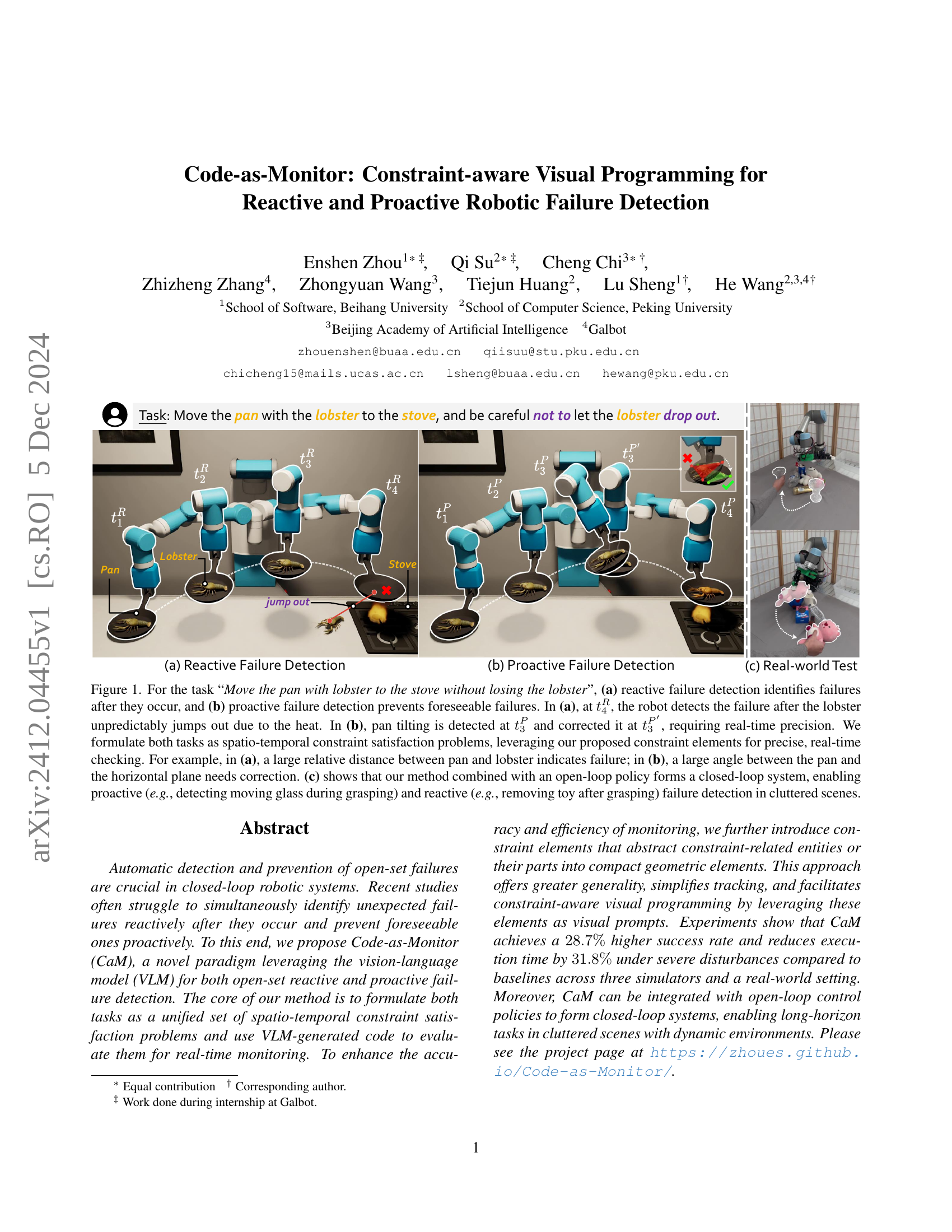
🔼 Figure 1 demonstrates different failure detection methods for a robotic task: moving a pan with a lobster to a stove without dropping the lobster. (a) shows reactive detection where a failure (lobster jumping out) is identified after it occurs. (b) illustrates proactive detection, where a potential failure (pan tilting) is detected and corrected before it causes a problem. Both scenarios use spatio-temporal constraints to identify and resolve issues. (c) shows the method integrated into a closed-loop system, which allows both proactive and reactive failure detection even in complex scenarios.
read the caption
Figure 1: For the task “Move the pan with lobster to the stove without losing the lobster”, (a) reactive failure detection identifies failures after they occur, and (b) proactive failure detection prevents foreseeable failures. In (a), at t4Rsubscriptsuperscript𝑡𝑅4t^{R}_{4}italic_t start_POSTSUPERSCRIPT italic_R end_POSTSUPERSCRIPT start_POSTSUBSCRIPT 4 end_POSTSUBSCRIPT, the robot detects the failure after the lobster unpredictably jumps out due to the heat. In (b), pan tilting is detected at t3Psubscriptsuperscript𝑡𝑃3t^{P}_{3}italic_t start_POSTSUPERSCRIPT italic_P end_POSTSUPERSCRIPT start_POSTSUBSCRIPT 3 end_POSTSUBSCRIPT and corrected it at t3P′subscriptsuperscript𝑡superscript𝑃′3t^{P^{\prime}}_{3}italic_t start_POSTSUPERSCRIPT italic_P start_POSTSUPERSCRIPT ′ end_POSTSUPERSCRIPT end_POSTSUPERSCRIPT start_POSTSUBSCRIPT 3 end_POSTSUBSCRIPT, requiring real-time precision. We formulate both tasks as spatio-temporal constraint satisfaction problems, leveraging our proposed constraint elements for precise, real-time checking. For example, in (a), a large relative distance between pan and lobster indicates failure; in (b), a large angle between the pan and the horizontal plane needs correction. (c) shows that our method combined with an open-loop policy forms a closed-loop system, enabling proactive (e.g., detecting moving glass during grasping) and reactive (e.g., removing toy after grasping) failure detection in cluttered scenes.
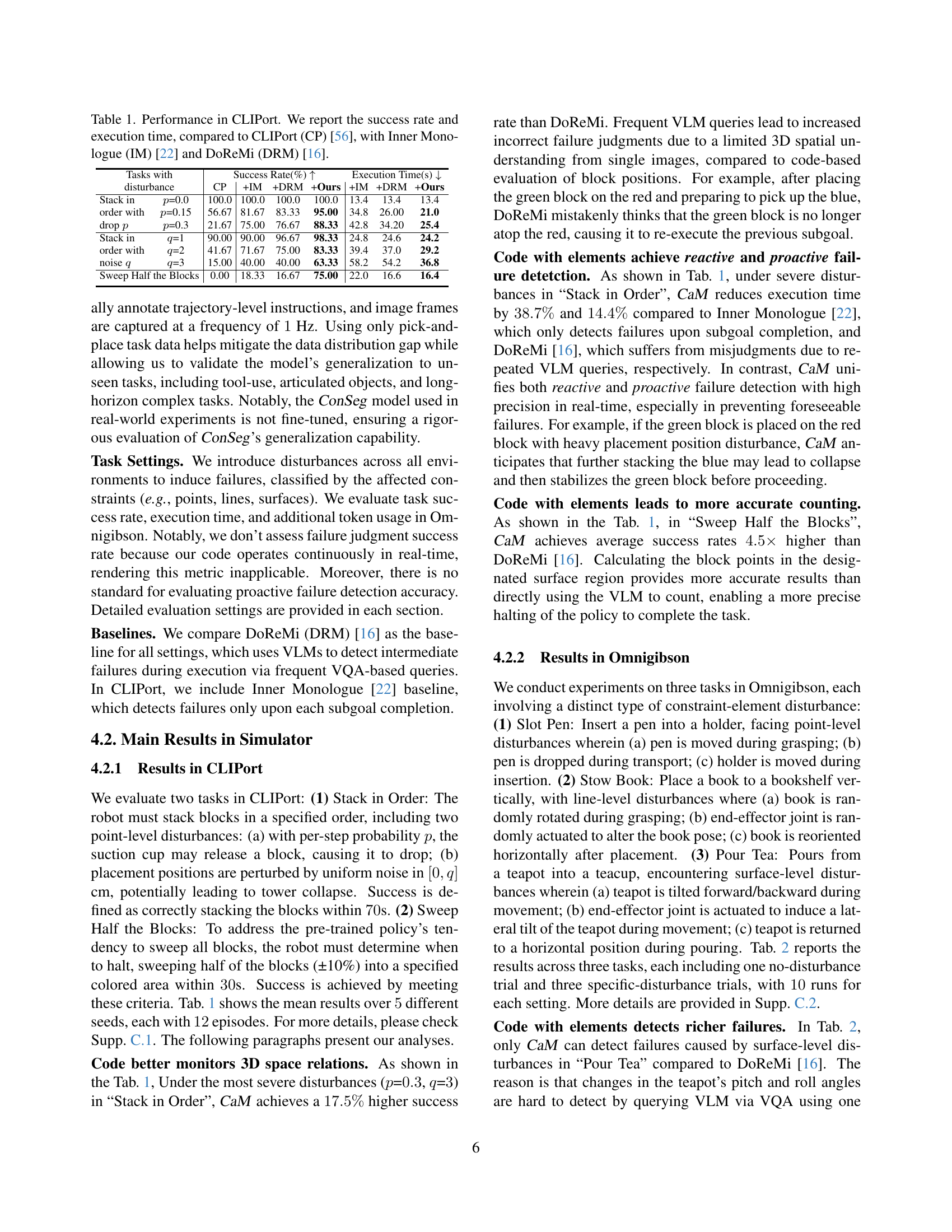
| Tasks with | Success Rate(%) ↑ | Execution Time(s) ↓ |
|---|---|---|
| disturbance | CP | +IM |
| Stack in p=0.0 | 100.0 | 100.0 |
| order with p=0.15 | 56.67 | 81.67 |
| drop p=0.3 | 21.67 | 75.00 |
| Stack in q=1 | 90.00 | 90.00 |
| order with q=2 | 41.67 | 71.67 |
| noise q=3 | 15.00 | 40.00 |
| Sweep Half the Blocks | 0.00 | 18.33 |
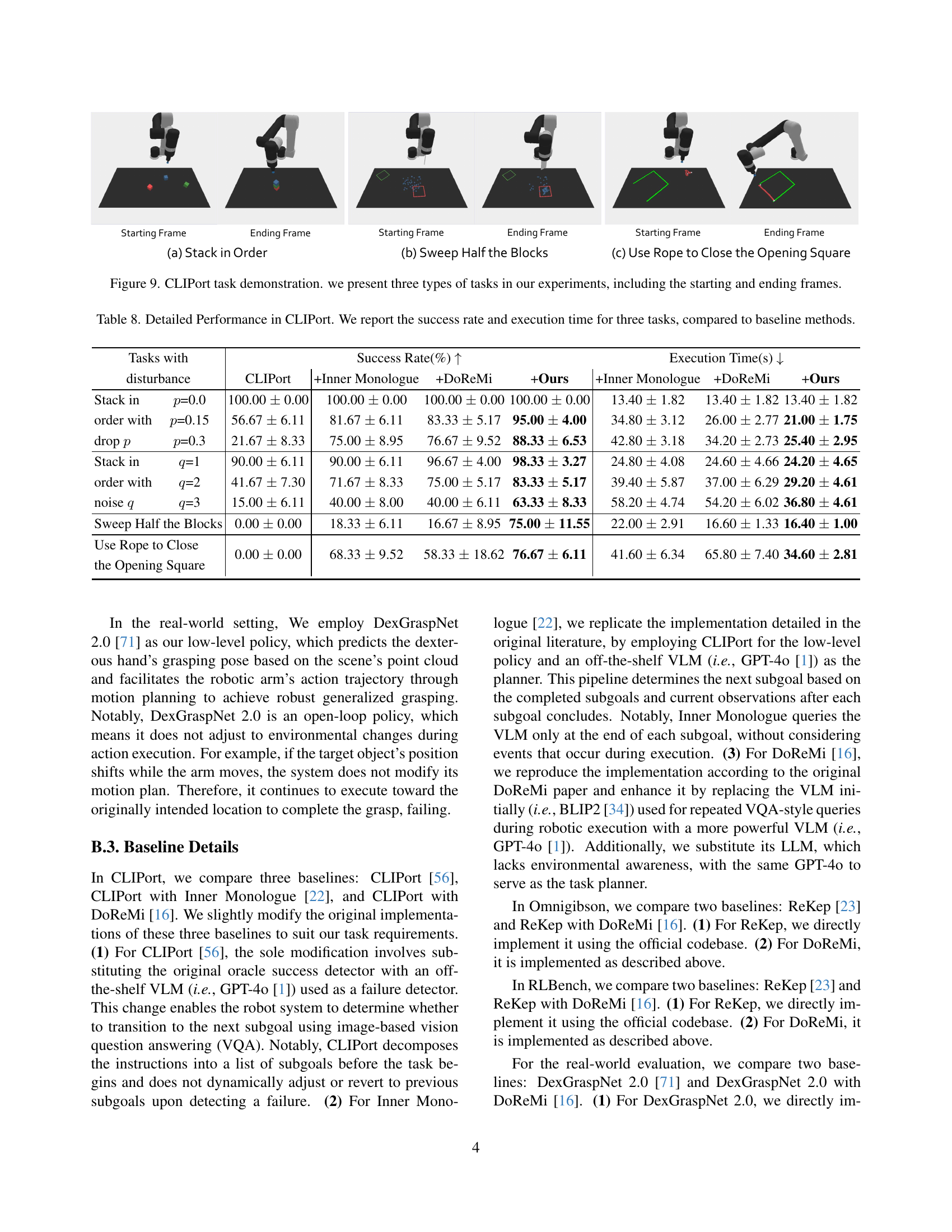
🔼 This table presents a comparison of the success rates and execution times for three manipulation tasks in the CLIPort simulator, achieved by four different methods: the original CLIPort method, CLIPort enhanced with Inner Monologue, CLIPort with DoReMi, and the proposed Code-as-Monitor method. The tasks involve stacking blocks, sweeping blocks, and using a rope to close a square opening, and each task is tested under varying levels of difficulty using different levels of introduced disturbances (probability of block dropping, noise level in block placement, etc.). The results highlight the performance improvements achieved by Code-as-Monitor in terms of both higher success rates and faster execution times.
read the caption
Table 1: Performance in CLIPort. We report the success rate and execution time, compared to CLIPort (CP) [56], with Inner Monologue (IM) [22] and DoReMi (DRM) [16].
In-depth insights#
Reactive Failure Detect#
Reactive failure detection, a critical aspect of robust robotic systems, focuses on identifying failures after they occur. This contrasts with proactive detection, which aims to prevent failures before they happen. A thoughtful reactive system requires real-time monitoring of the robot’s state and environment to quickly identify deviations from expected behavior. Sensor data plays a crucial role in this process, enabling rapid identification of unexpected events like object drops or collisions. Effective reactive detection necessitates a well-defined set of failure criteria, allowing the system to distinguish between normal operational variations and actual failures. Furthermore, a successful system should incorporate immediate feedback mechanisms such as re-planning or corrective actions to mitigate the consequences of detected failures. The success of reactive failure detection is ultimately judged by its ability to minimize downtime and prevent catastrophic system failures. The design of a robust and effective reactive failure detection system requires careful consideration of multiple factors. Accuracy, speed, and resilience are vital characteristics. Balancing these factors is essential for creating a truly reliable and safe robotic system.
Visual Programming#
The concept of ‘Visual Programming’ in the context of robotics, as discussed in the research paper, represents a significant shift towards more intuitive and efficient methods for robot control and failure detection. It leverages the power of vision-language models (VLMs) to translate high-level task instructions and visual observations into executable code that directly monitors spatio-temporal constraints. This approach moves beyond traditional textual programming, offering a more accessible and user-friendly interface for designing robot behaviors. The use of constraint elements, abstract geometric representations of relevant entities, further simplifies the visual programming process. By enabling real-time constraint monitoring through code evaluation, visual programming offers increased efficiency and accuracy in both reactive and proactive failure detection, adapting to unseen situations with greater flexibility than text-based methods alone. The integration of visual programming with open-loop policies allows for more robust and adaptable closed-loop systems in complex dynamic environments. In essence, visual programming is not just a novel technique; it’s a paradigm shift that profoundly affects how robots are programmed and how failures are addressed.
Constraint Elements#
The concept of ‘Constraint Elements’ appears crucial for bridging the gap between high-level task instructions and low-level robot control. These elements act as intermediaries, abstracting complex real-world entities and their spatial relationships into simpler geometric representations (points, lines, surfaces). This abstraction is key for several reasons: efficiency, enabling real-time monitoring without the computational overhead of processing raw sensory data; generalization, allowing the system to adapt to variations in object appearances and environmental conditions; and interpretability, simplifying the task of specifying and verifying constraints for both reactive and proactive failure detection. Visual programming is facilitated by representing these elements as visual prompts, making the monitoring process more intuitive and easier to design. By leveraging spatio-temporal constraints on these elements, the system can effectively and precisely detect failures, whether anticipated or unexpected, significantly improving the robustness and reliability of closed-loop robotic systems.
Real-world Testing#
Real-world testing of robotic systems is crucial for validating the effectiveness and robustness of algorithms and control policies developed in simulated environments. A successful real-world test should demonstrate the system’s ability to handle unexpected events and uncertainties inherent in unstructured environments. The challenges of real-world testing include the difficulty of replicating the complexity and variability of real-world conditions in simulation, the cost and time required to conduct extensive experiments, and the safety implications of deploying robots in uncontrolled settings. A well-designed real-world test should consider various factors, such as the choice of test environment, the types of tasks performed, the presence of disturbances or failures, and the metrics used to evaluate performance. The results of the testing phase should provide valuable insights into the strengths and weaknesses of the system, leading to improvements in design and implementation. Data collected from real-world testing is invaluable for further refinement and validation of the system, potentially leading to more robust and reliable robotic systems suitable for deployment in a variety of real-world applications. Ideally, the results will contribute to a better understanding of how to translate algorithms effectively from simulation to the real world, bridging the gap between theory and practice.
Future Directions#
Future research directions for this work could explore several promising avenues. Extending the constraint element framework to encompass a wider range of failure modes, particularly those involving subtle force interactions or nuanced sensory data (e.g., sounds, temperature changes), is crucial. This could involve incorporating more sophisticated geometric primitives or integrating multimodal sensing capabilities. Improving the robustness and generalization of the VLM-generated code is essential. Research on techniques for mitigating hallucinations and enhancing the reliability of code execution in dynamic real-world scenarios should be prioritized. Furthermore, exploring the integration with advanced planning and control algorithms would enable the development of more sophisticated closed-loop systems capable of handling long-horizon tasks in complex and unpredictable environments. Finally, benchmarking the system on a wider variety of robotic tasks and environments, coupled with a thorough comparative analysis against state-of-the-art methods, would provide valuable insights into the overall performance and limitations of the proposed approach.
More visual insights#
More on figures

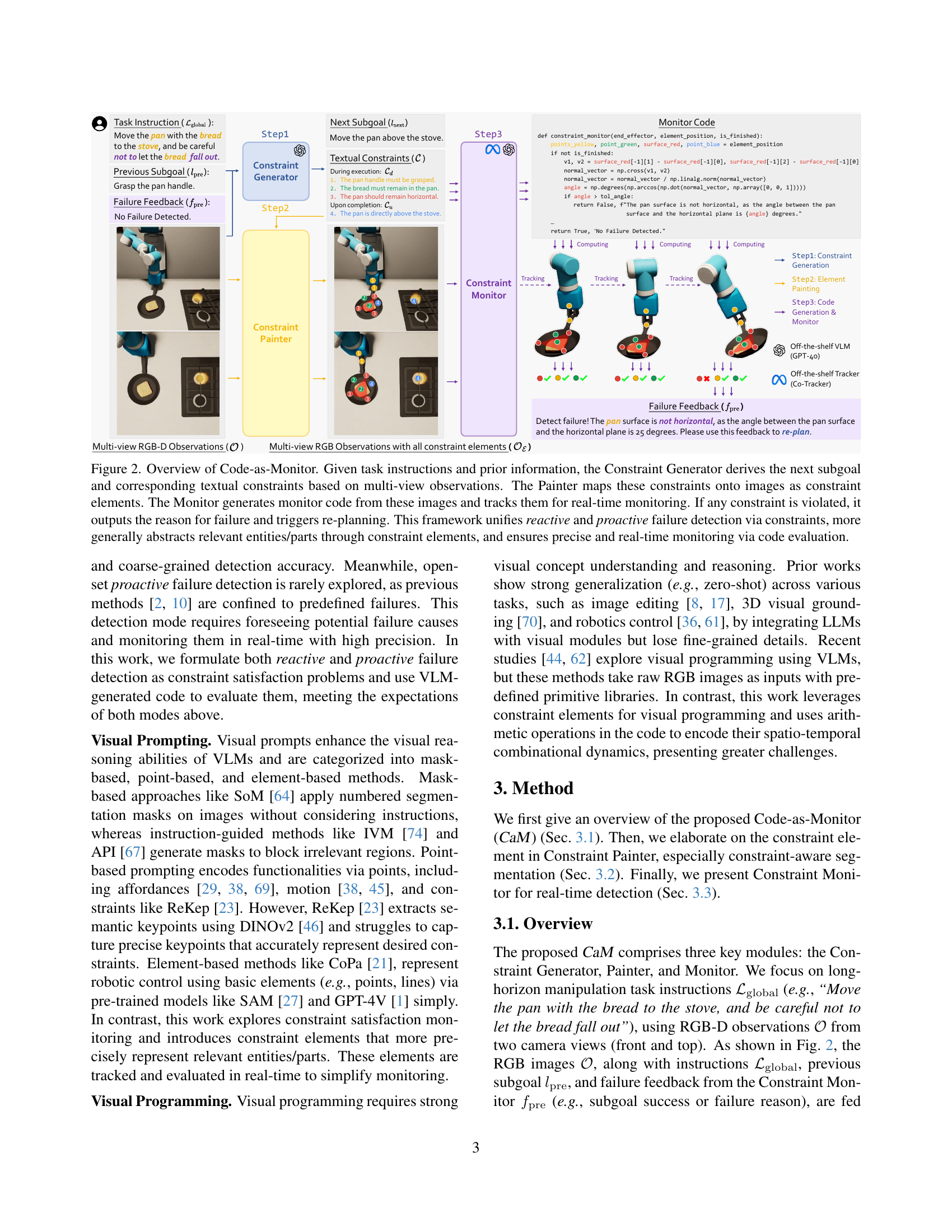
🔼 The figure illustrates the Code-as-Monitor (CaM) framework, which unifies reactive and proactive failure detection in robotics. Given a task instruction (e.g., ‘Move the pan with the bread to the stove without dropping the bread’), the Constraint Generator analyzes multi-view observations and determines the next subgoal and its associated textual constraints. The Painter module converts these textual constraints into visual representations (constraint elements) overlaid on the images. The Monitor module then uses these visual elements to generate and execute code that performs real-time monitoring for constraint satisfaction. If a constraint is violated, the Monitor outputs the reason for failure, triggering re-planning. The use of constraint elements simplifies the monitoring process and enhances the generality and real-time performance of the system.
read the caption
Figure 2: Overview of Code-as-Monitor. Given task instructions and prior information, the Constraint Generator derives the next subgoal and corresponding textual constraints based on multi-view observations. The Painter maps these constraints onto images as constraint elements. The Monitor generates monitor code from these images and tracks them for real-time monitoring. If any constraint is violated, it outputs the reason for failure and triggers re-planning. This framework unifies reactive and proactive failure detection via constraints, more generally abstracts relevant entities/parts through constraint elements, and ensures precise and real-time monitoring via code evaluation.

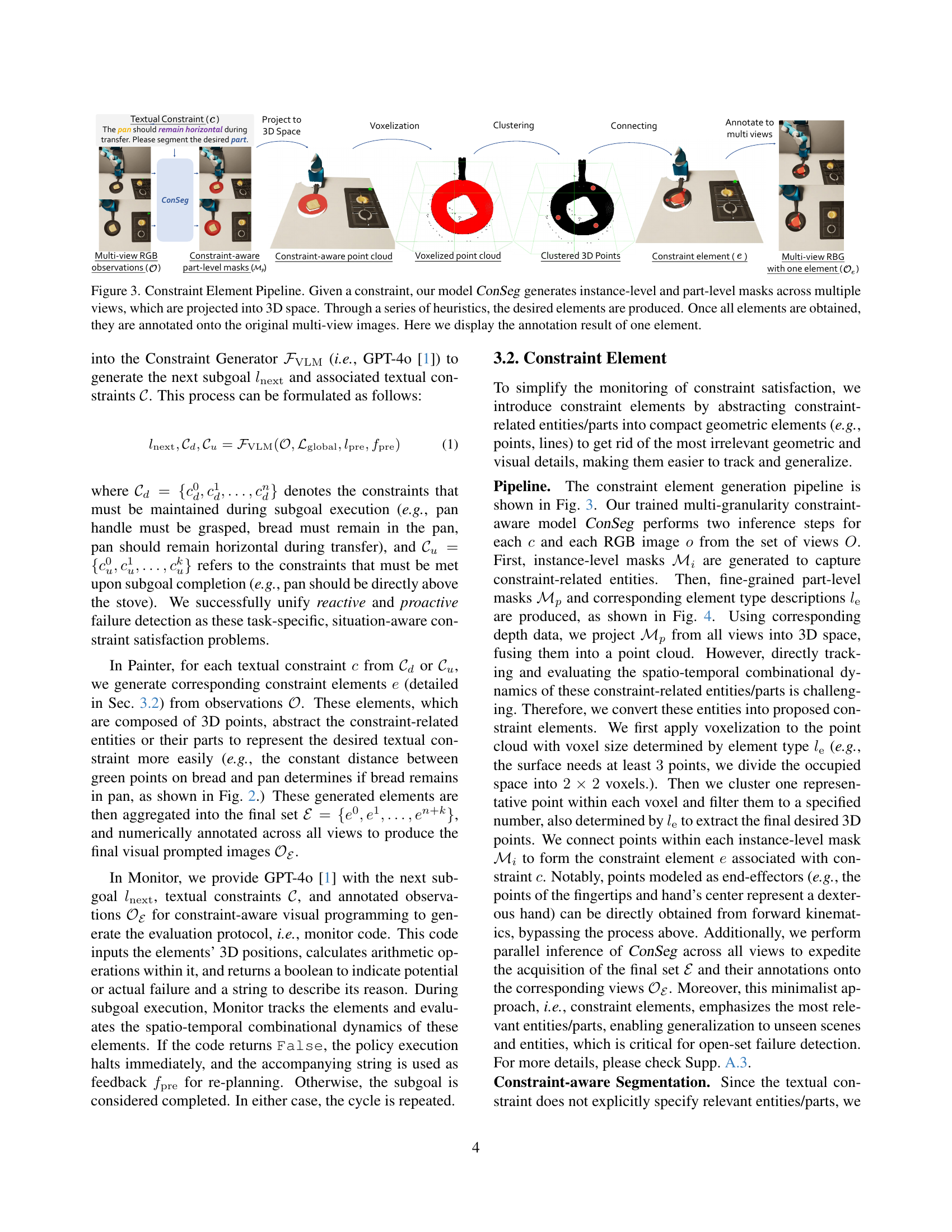
🔼 The figure illustrates the process of generating constraint elements from multi-view images. First, the ConSeg model generates instance-level and part-level masks from multiple camera views. These masks are then projected into 3D space. A series of heuristics are applied to the 3D point cloud to identify and extract the desired constraint elements. Finally, these elements are annotated back onto the original multi-view images for visualization and use in subsequent monitoring tasks. The figure shows the annotation result for a single constraint element.
read the caption
Figure 3: Constraint Element Pipeline. Given a constraint, our model ConSeg generates instance-level and part-level masks across multiple views, which are projected into 3D space. Through a series of heuristics, the desired elements are produced. Once all elements are obtained, they are annotated onto the original multi-view images. Here we display the annotation result of one element.

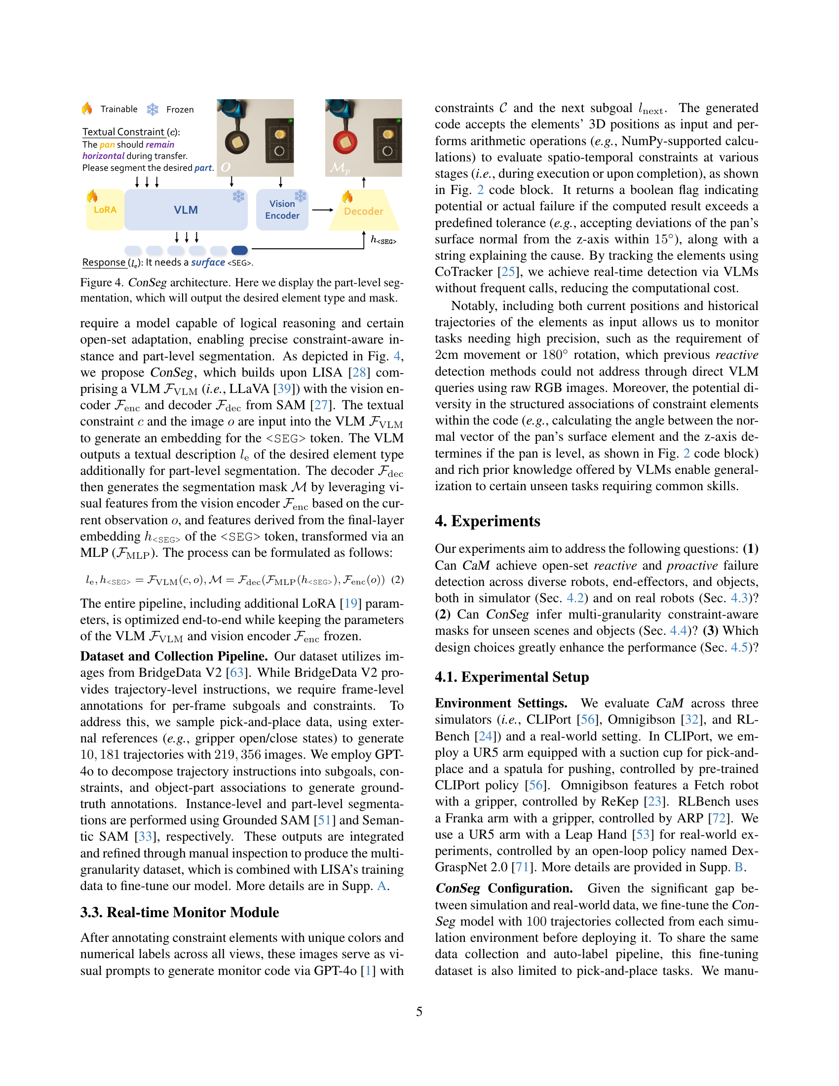
🔼 The figure showcases the architecture of ConSeg, a model designed for constraint-aware part-level segmentation. It takes as input a textual constraint describing the desired object part and a corresponding image. The model processes the image via a vision encoder and uses a vision-language model (VLM) to generate an embedding based on the textual constraint and the visual features. This embedding is used by a decoder to produce the segmentation mask identifying the specific part of the object that satisfies the constraint. The output includes both the mask and a description (element type) of the segmented part. This method ensures precise segmentation of only the relevant parts required for constraint satisfaction, aiding in visual programming.
read the caption
Figure 4: ConSeg architecture. Here we display the part-level segmentation, which will output the desired element type and mask.

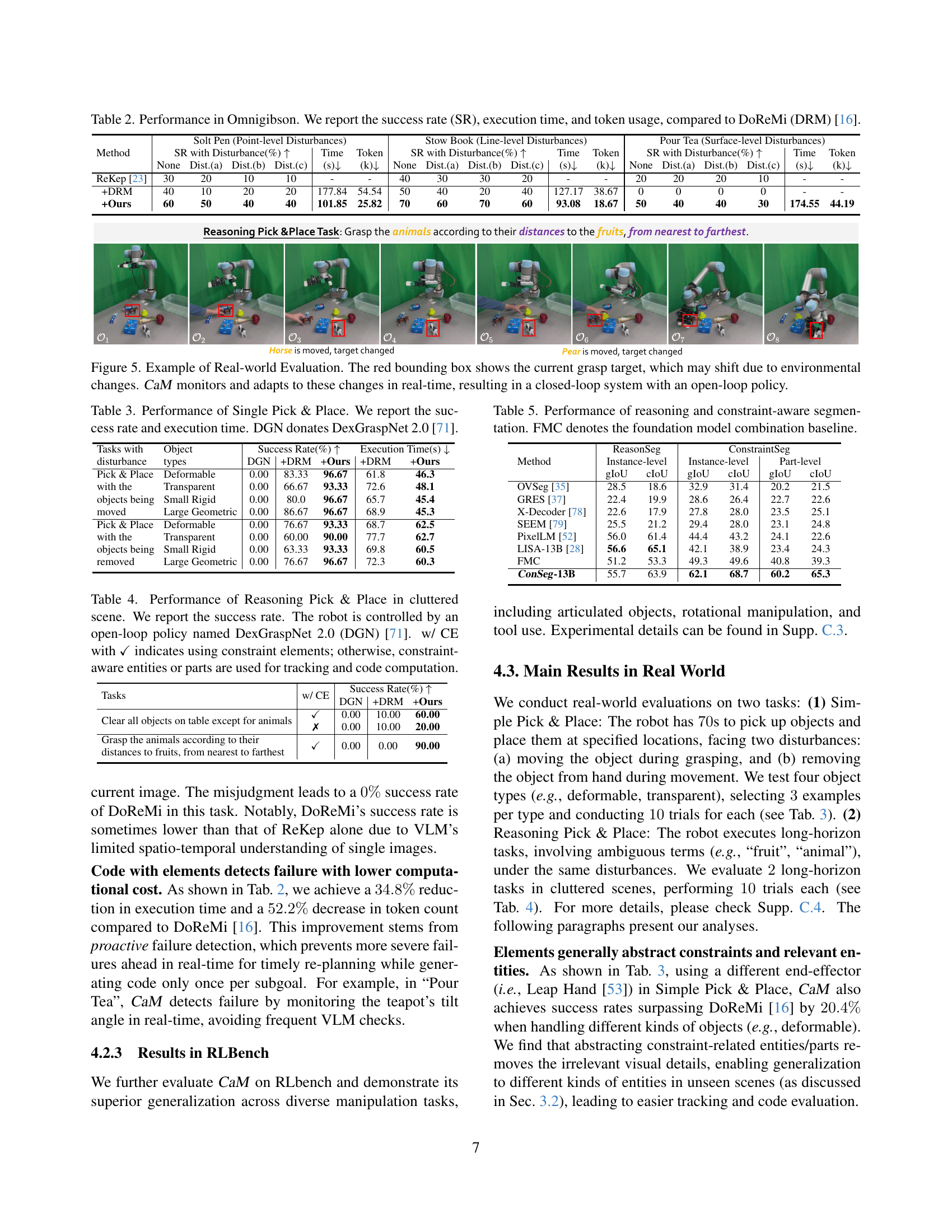
🔼 The figure showcases a real-world robotic manipulation task where the robot’s grasp target dynamically changes due to environmental factors. The red bounding box highlights this shifting target. The Code-as-Monitor (CaM) system actively tracks these changes in real-time and adapts accordingly. This creates a closed-loop system, effectively combining CaM’s reactive and proactive failure detection with an existing open-loop control policy.
read the caption
Figure 5: Example of Real-world Evaluation. The red bounding box shows the current grasp target, which may shift due to environmental changes. CaM monitors and adapts to these changes in real-time, resulting in a closed-loop system with an open-loop policy.

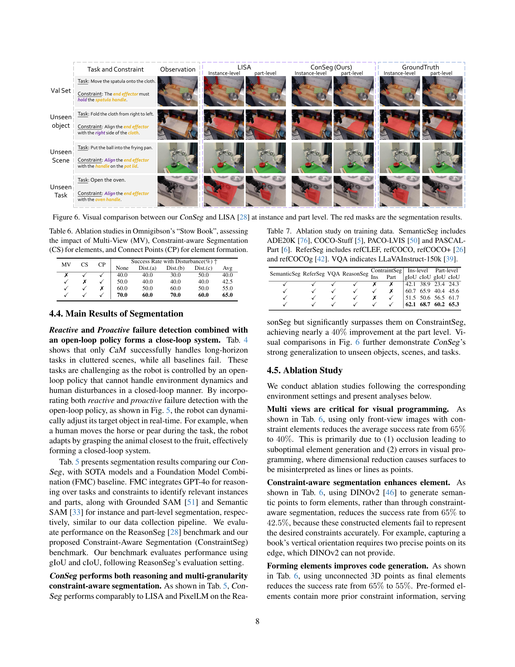
🔼 Figure 6 presents a detailed comparison of the segmentation results produced by the proposed ConSeg model and the LISA [28] model. It showcases both instance-level and part-level segmentations. The visual comparison allows for a direct assessment of the accuracy and granularity of each model’s output in identifying objects and their constituent parts within the image. Red masks highlight the segmentation results generated by both methods, enabling an easy side-by-side comparison of their performance. This comparative analysis highlights the advantages of the proposed ConSeg model in terms of accuracy and detailed part segmentation.
read the caption
Figure 6: Visual comparison between our ConSeg and LISA [28] at instance and part level. The red masks are the segmentation results.

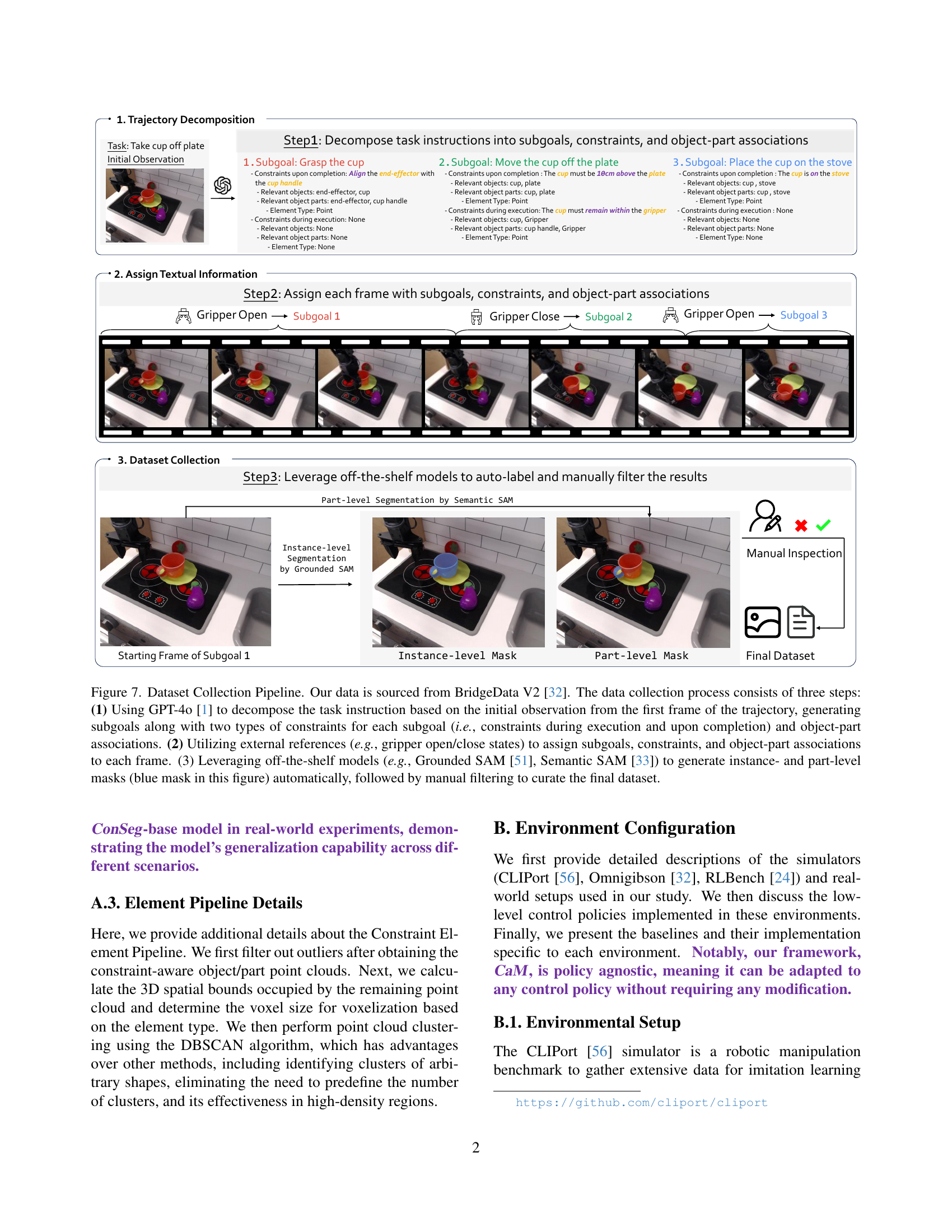
🔼 This figure illustrates the three-step process for collecting the dataset used in the paper. First, GPT-4 is used to analyze each trajectory from the BridgeData V2 dataset [32], breaking down the task instructions into individual subgoals, identifying constraints (both during execution and upon completion), and defining the object-part relationships involved in each subgoal. Second, using external information, such as gripper states, each frame of the trajectory is linked to the corresponding subgoal, constraints, and object-part associations. Finally, pre-trained models (Grounded SAM [51] and Semantic SAM [33]) automatically generate instance and part-level segmentation masks. Manual review and filtering are then used to refine the dataset, removing any errors or low-quality annotations.
read the caption
Figure 7: Dataset Collection Pipeline. Our data is sourced from BridgeData V2 [32]. The data collection process consists of three steps: (1) Using GPT-4o [1] to decompose the task instruction based on the initial observation from the first frame of the trajectory, generating subgoals along with two types of constraints for each subgoal (i.e., constraints during execution and upon completion) and object-part associations. (2) Utilizing external references (e.g., gripper open/close states) to assign subgoals, constraints, and object-part associations to each frame. (3) Leveraging off-the-shelf models (e.g., Grounded SAM [51], Semantic SAM [33]) to generate instance- and part-level masks (blue mask in this figure) automatically, followed by manual filtering to curate the final dataset.

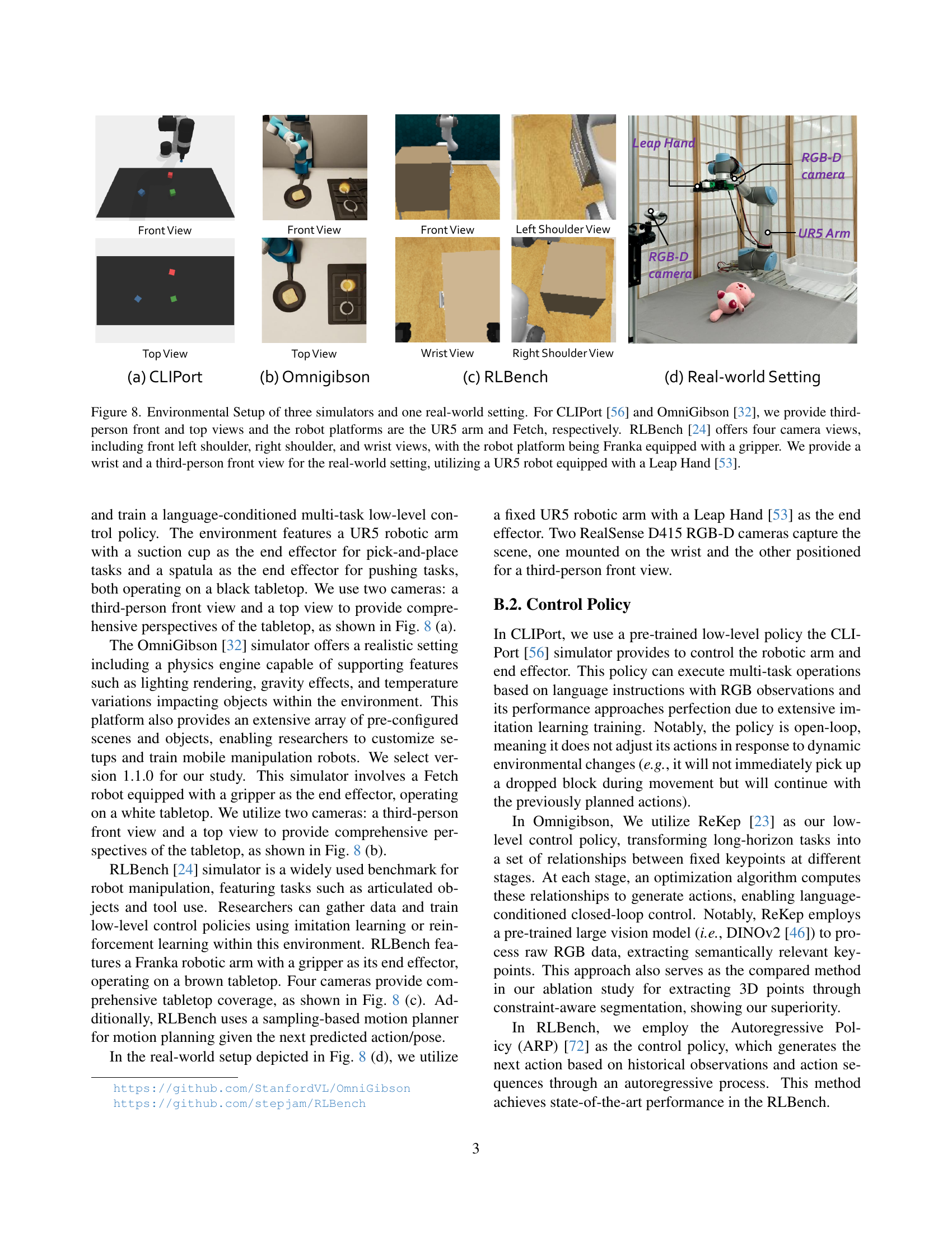
🔼 Figure 8 illustrates the experimental setups used in the paper, encompassing three simulation environments (CLIPort, OmniGibson, RLBench) and a real-world setting. The simulation environments are depicted with their respective robot arms (UR5 for CLIPort and OmniGibson, Franka for RLBench), camera views (third-person front and top for CLIPort and OmniGibson; front left shoulder, right shoulder, wrist for RLBench), and the objects being manipulated. The real-world setup shows a UR5 arm with a Leap Hand, utilizing both wrist and third-person front views. This figure highlights the consistency of the experimental methodology across simulations and real-world testing.
read the caption
Figure 8: Environmental Setup of three simulators and one real-world setting. For CLIPort [56] and OmniGibson [32], we provide third-person front and top views and the robot platforms are the UR5 arm and Fetch, respectively. RLBench [24] offers four camera views, including front left shoulder, right shoulder, and wrist views, with the robot platform being Franka equipped with a gripper. We provide a wrist and a third-person front view for the real-world setting, utilizing a UR5 robot equipped with a Leap Hand [53].

🔼 This figure shows example image sequences from three different tasks in the CLIPort environment. Each task demonstrates the robot performing a manipulation action from start to finish. The purpose is to illustrate the variety of manipulation tasks used to evaluate the proposed approach. The three tasks are: (a) Stack in Order, (b) Sweep Half the Blocks, and (c) Use Rope to Close the Opening Square.
read the caption
Figure 9: CLIPort task demonstration. we present three types of tasks in our experiments, including the starting and ending frames.

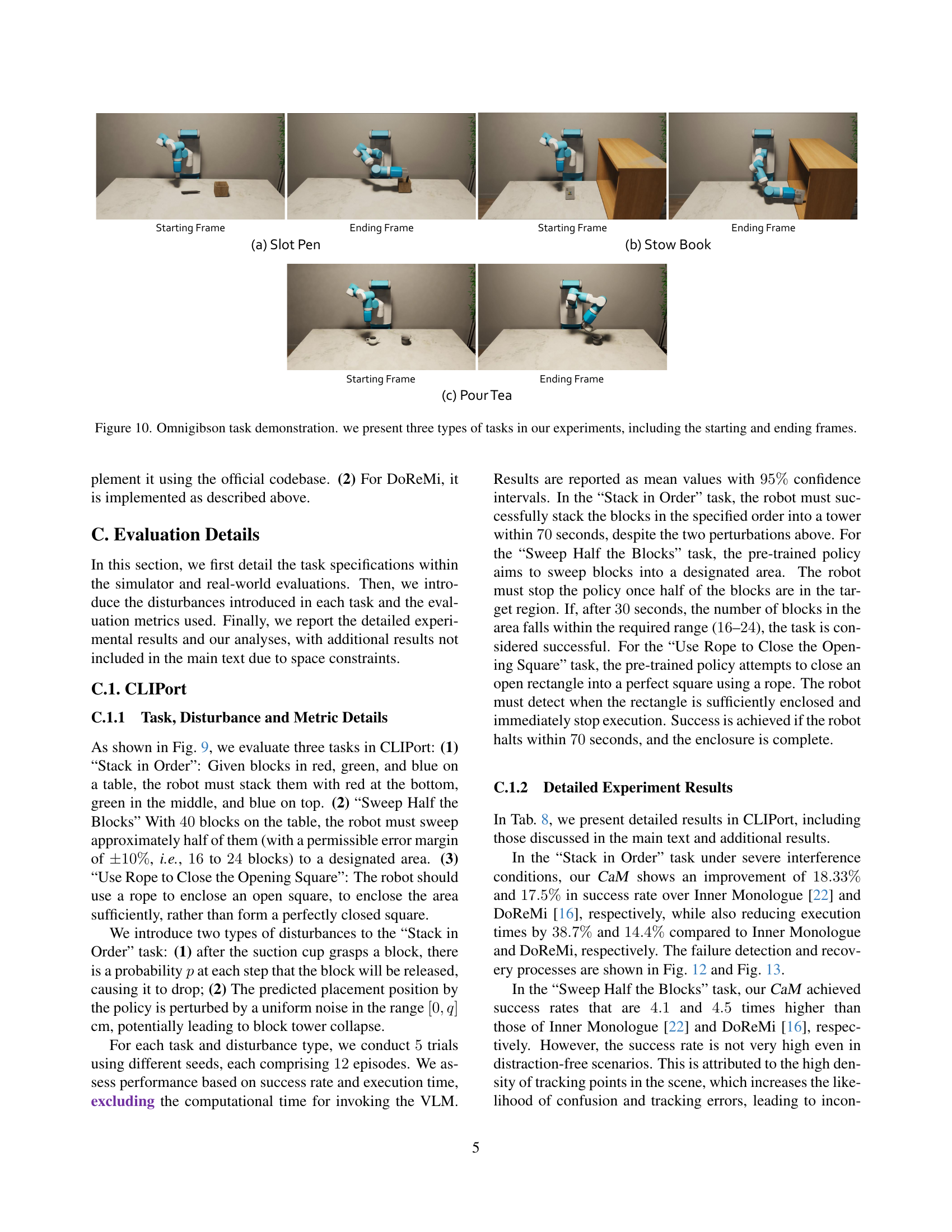
🔼 This figure showcases three distinct robotic manipulation tasks from the Omnigibson simulator used in the paper’s experiments. Each task is visually represented with a sequence of images showing the initial and final states. The tasks demonstrate the diversity of manipulation challenges addressed by the proposed method.
read the caption
Figure 10: Omnigibson task demonstration. we present three types of tasks in our experiments, including the starting and ending frames.

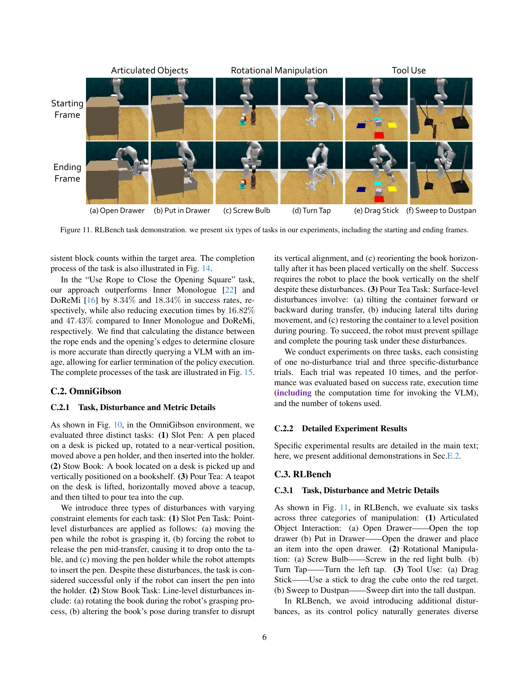
🔼 This figure showcases six diverse manipulation tasks from the RLBench benchmark, illustrating the types of challenges addressed in the paper. Each task includes a starting and ending frame, providing a visual representation of the robot’s actions and the complexity involved. The tasks encompass a range of manipulation skills, including articulated object interactions (e.g., opening drawers, inserting objects), rotational manipulations (e.g., turning taps, screwing bulbs), and tool use (e.g., dragging with a stick, sweeping with a dustpan).
read the caption
Figure 11: RLBench task demonstration. we present six types of tasks in our experiments, including the starting and ending frames.
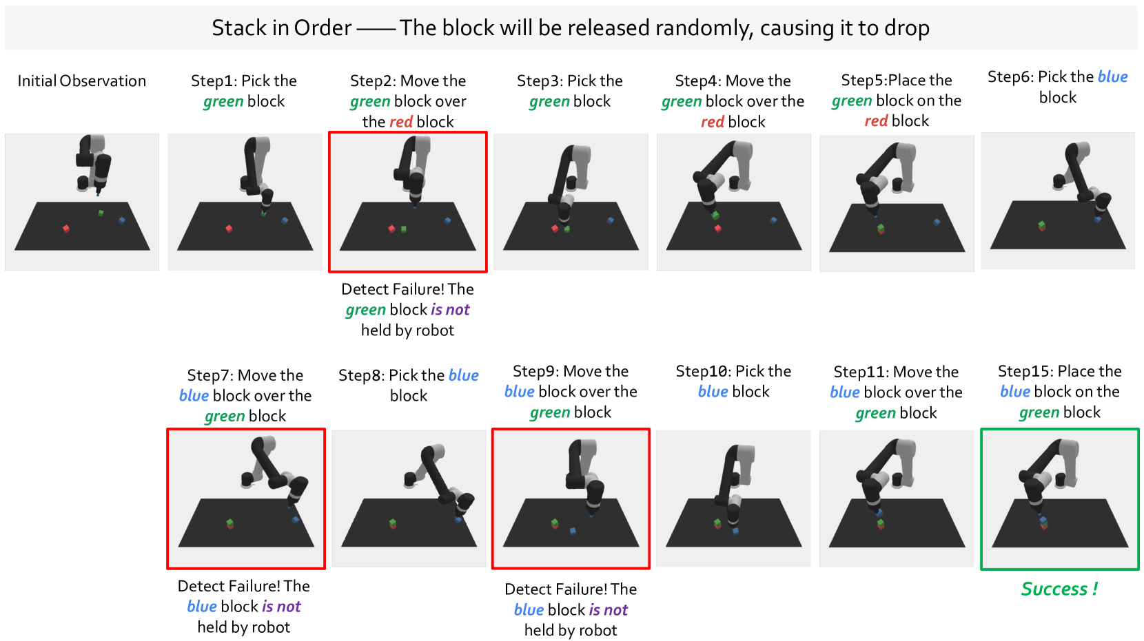
🔼 This figure demonstrates the ‘Stack in Order’ task, where the robot stacks blocks in a specific order (red, green, blue). The experiment introduces a disturbance: the placement position of each block is randomly perturbed by a small amount (up to q cm). The figure showcases how the proposed framework detects when a block is not placed correctly (reactive failure detection). Red boxes highlight these failures, indicating that the robot failed to satisfy the specified spatial constraints. The framework’s ability to recover from these failures is also demonstrated (proactive failure detection), with green boxes marking successful placements after correction. This illustrates the system’s ability to address errors and ensure successful task completion.
read the caption
Figure 12: Demonstration of “Stack in Order”. We show how our framework detects failures and assists in recovery when the placement positions predicted by the policy for the “Stack in Order” task are subject to a uniform [0,q]0𝑞[0,q][ 0 , italic_q ] cm interference. Red boxes indicate the occurrence of failures, while green boxes signify successful task execution.

🔼 This figure demonstrates the ‘Stack in Order’ task, where a robot stacks blocks. Failures are simulated by randomly releasing blocks (with probability p) from the robot’s suction cup. The figure shows the robot’s actions, highlighting failures (red boxes) and successful steps (green boxes). The framework’s ability to detect failures and recover is showcased.
read the caption
Figure 13: Demonstration of “Stack in Order”. We show how our framework performs failure detection and aids in recovery when, in the “Stack in Order” task, there is a probability p𝑝pitalic_p that blocks will fall due to being released by the robot’s suction cup at each step. Red boxes indicate the occurrence of failures, while green boxes signify successful task execution.

🔼 The figure shows a comparison of the proposed method and a baseline method (DoReMi) for the task of sweeping half of the blocks into a specified area. The proposed method accurately counts the number of blocks in the area and stops the robot when the task is completed, preventing task failure. In contrast, the baseline method fails to stop the robot in time, causing it to continue sweeping blocks beyond the specified number, which results in task failure. Red boxes highlight instances of failure, whereas green boxes indicate successful task execution.
read the caption
Figure 14: Demonstration of “Sweep Half the Blocks” and comparison to baseline. We show our framework can precisely count the blocks within a specified area and timely halts the policy execution to complete the task. In contrast, DoReMi [16] fails to stop the policy execution in time, leading to task failure. Red boxes indicate the occurrence of failures, while green boxes signify successful task execution.

🔼 The figure demonstrates a comparison between the proposed Code-as-Monitor (CaM) framework and the DoReMi baseline in performing the ‘Use Rope to Close the Opening Square’ task. CaM effectively detects when the rope successfully closes the square and stops the robot’s actions promptly, completing the task efficiently. In contrast, DoReMi, while eventually successful, fails to stop the robot in a timely manner, resulting in a significant increase in execution time. The use of red and green boxes in the figure highlight task failures and successes, respectively, for a clear visual comparison of the two methods.
read the caption
Figure 15: Demonstration of “Use Rope to Close the Opening Square” and comparison to baseline. We show that our framework effectively detects when the rope closes the opening square and promptly stops the policy execution to complete the task successfully. Conversely, DoReMi fails to halt the policy execution on time; although it eventually succeeds in closing the opening, the excessive execution time results in task failure. Red boxes indicate the occurrence of failures, while green boxes signify successful task execution.

🔼 This figure demonstrates the ‘Slot Pen’ task, showing how the Code-as-Monitor framework handles point-level disturbances. The sequence of images illustrates the robot’s actions, highlighting failures (red boxes), successful recovery after a failure (light green boxes), and successful task completion (dark green boxes). Point-level disturbances include actions such as the pen moving unexpectedly or dropping during manipulation. The figure showcases how the system identifies these failures and takes corrective actions to successfully complete the task.
read the caption
Figure 16: Demonstration of “Slot Pen”. We show how our framework detects failures and assists in recovery when facing point-level disturbances. Red boxes indicate the occurrence of failures, light green indicates the recovery with subgoal success and dark green boxes signify successful task execution.
🔼 The figure showcases the framework’s ability to detect and handle failures during the ‘Stow Book’ task, specifically when line-level disturbances occur. The process is illustrated step-by-step, highlighting the different stages. Red boxes highlight instances where the system identifies a failure; light green boxes indicate successful recovery after a failure; dark green boxes indicate successful task completion without encountering any failures.
read the caption
Figure 17: Demonstration of “Stow Book”. We show how our framework detects failures and assists in recovery when facing line-level disturbances. Red boxes indicate the occurrence of failures, light green indicates the recovery with subgoal success and dark green boxes signify successful task execution.

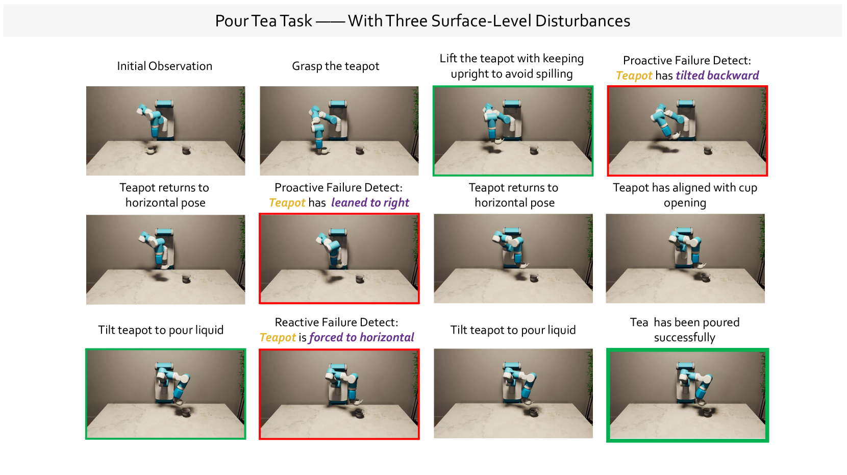
🔼 The figure showcases the different stages involved in the “Pour Tea” task, highlighting the capabilities of the proposed framework in handling surface-level disturbances. The initial state shows the robot and the objects involved. Subsequent steps demonstrate the robot’s actions, with red boxes indicating instances where failures were detected. The light green boxes illustrate successful recovery after detecting failures, whereas the dark green boxes represent successful task completion without any failure detection.
read the caption
Figure 18: Demonstration of “Pour Tea”. We show how our framework detects failures and assists in recovery when facing surface-level disturbances. Red boxes indicate the occurrence of failures, light green indicates the recovery with subgoal success and dark green boxes signify successful task execution.

🔼 The figure demonstrates the robot performing the task of clearing all objects from a table except for the animals. The robot uses a combination of reactive and proactive failure detection. Reactive detection addresses unexpected issues, like a human removing an object during the robot’s grasp. Proactive detection anticipates potential problems, such as a human moving an object while the robot is trying to grasp it. By anticipating and correcting for these issues, the system improves the task’s success rate and reduces the time needed for completion.
read the caption
Figure 19: Demonstration of “Clear all objects on the table except for animals”. We show that our framework achieves both reactive failure detection (e.g., detecting unexpected failures when humans remove objects from the robot’s grasp) and proactive failure detection (e.g., identifying target object movement during grasping to prevent foreseeable failures). This effectively enhances the task success rate and reduces the execution time.

🔼 This figure visualizes the results of applying constraint-aware image segmentation to the RoboFail dataset [41]. The RoboFail dataset contains images of robotic manipulation tasks with various failure scenarios. The constraint-aware segmentation model, a key component of the Code-as-Monitor system presented in the paper, is designed to identify and segment specific regions (or elements) in the image that are relevant to the fulfillment of task constraints. Because the RoboFail dataset was not used in training the model, this visualization demonstrates the model’s ability to generalize to unseen data and perform accurate segmentation of task-relevant elements even in novel scenarios.
read the caption
Figure 20: Visualization of constraint-aware segmentation for the RoboFail Dataset [41]. This dataset is not included in the training data.

🔼 Figure 21 visualizes the results of applying constraint-aware segmentation to the Open6DOF benchmark dataset [11], which was not part of the model’s training data. The figure showcases how the model identifies and segments relevant entities and parts of objects for various tasks (e.g., grasping, placing), highlighting its ability to generalize to unseen data and situations.
read the caption
Figure 21: Visualization of constraint-aware segmentation for the Open6DOF [11]. This dataset is not included in the training data.

🔼 This figure visualizes the results of applying constraint-aware segmentation to images from the RT-1 dataset [3], which is a real-world robotic manipulation dataset. The RT-1 dataset was not used during the training of the constraint-aware segmentation model. The visualization shows the model’s ability to identify and segment relevant objects and parts in images that were not seen during the model’s training, demonstrating its generalization capabilities to new, unseen data. Each sub-figure presents a task from the dataset and the resulting segmentation masks generated by the model, highlighting the model’s ability to accurately identify and isolate objects and parts based on the given constraints.
read the caption
Figure 22: Visualization of constraint-aware segmentation for the RT-1 dataset [3]. This dataset is not included in the training data.

🔼 The figure displays the results of applying constraint-aware segmentation to the Omnigibson simulator. It shows the instance-level and part-level segmentations for various tasks within the simulator. Each task is decomposed into subgoals and constraints, and the visualizations highlight how the model identifies and segments the relevant objects and their parts according to those constraints.
read the caption
Figure 23: Visualization of constraint-aware segmentation for the Omnigibsom simulator.
More on tables
| Method | Solt Pen (Point-level Disturbances) | Stow Book (Line-level Disturbances) | Pour Tea (Surface-level Disturbances) | |||||||||||||||
|---|---|---|---|---|---|---|---|---|---|---|---|---|---|---|---|---|---|---|
| SR with Disturbance(%) ↑ | Time | Token | SR with Disturbance(%) ↑ | Time | Token | SR with Disturbance(%) ↑ | Time | Token | ||||||||||
| — | — | — | — | — | — | — | — | — | — | — | — | — | — | — | — | — | — | — |
| ReKep [23] | 30 | 20 | 10 | 10 | - | - | 40 | 30 | 30 | 20 | - | - | 20 | 20 | 20 | 10 | - | - |
| +DRM | 40 | 10 | 20 | 20 | 177.84 | 54.54 | 50 | 40 | 20 | 40 | 127.17 | 38.67 | 0 | 0 | 0 | 0 | - | - |
| +Ours | 60 | 50 | 40 | 40 | 101.85 | 25.82 | 70 | 60 | 70 | 60 | 93.08 | 18.67 | 50 | 40 | 40 | 30 | 174.55 | 44.19 |
🔼 This table presents a comparison of the performance of the Code-as-Monitor (CaM) system against a baseline method (DoReMi) [16] on three manipulation tasks within the Omnigibson simulator. The tasks are designed to evaluate the system’s ability to handle failures in a variety of situations, including point-level, line-level and surface-level disturbances. For each task and disturbance condition, the table shows the success rate (SR), execution time, and the number of tokens used by each system. The success rate indicates the percentage of trials in which the task was successfully completed. The execution time measures how long it took for the robot to complete the task. Token usage is a measure of the computational cost associated with running each system.
read the caption
Table 2: Performance in Omnigibson. We report the success rate (SR), execution time, and token usage, compared to DoReMi (DRM) [16].
| Tasks with | Object | Success Rate(%) ↑ | Success Rate(%) ↑ | Success Rate(%) ↑ | Execution Time(s) ↓ | Execution Time(s) ↓ |
|---|---|---|---|---|---|---|
| disturbance | types | DGN | +DRM | +Ours | +DRM | +Ours |
| Pick & Place | Deformable | 0.00 | 83.33 | 96.67 | 61.8 | 46.3 |
| with the | Transparent | 0.00 | 66.67 | 93.33 | 72.6 | 48.1 |
| objects being | Small Rigid | 0.00 | 80.0 | 96.67 | 65.7 | 45.4 |
| moved | Large Geometric | 0.00 | 86.67 | 96.67 | 68.9 | 45.3 |
| Pick & Place | Deformable | 0.00 | 76.67 | 93.33 | 68.7 | 62.5 |
| with the | Transparent | 0.00 | 60.00 | 90.00 | 77.7 | 62.7 |
| objects being | Small Rigid | 0.00 | 63.33 | 93.33 | 69.8 | 60.5 |
| removed | Large Geometric | 0.00 | 76.67 | 96.67 | 72.3 | 60.3 |
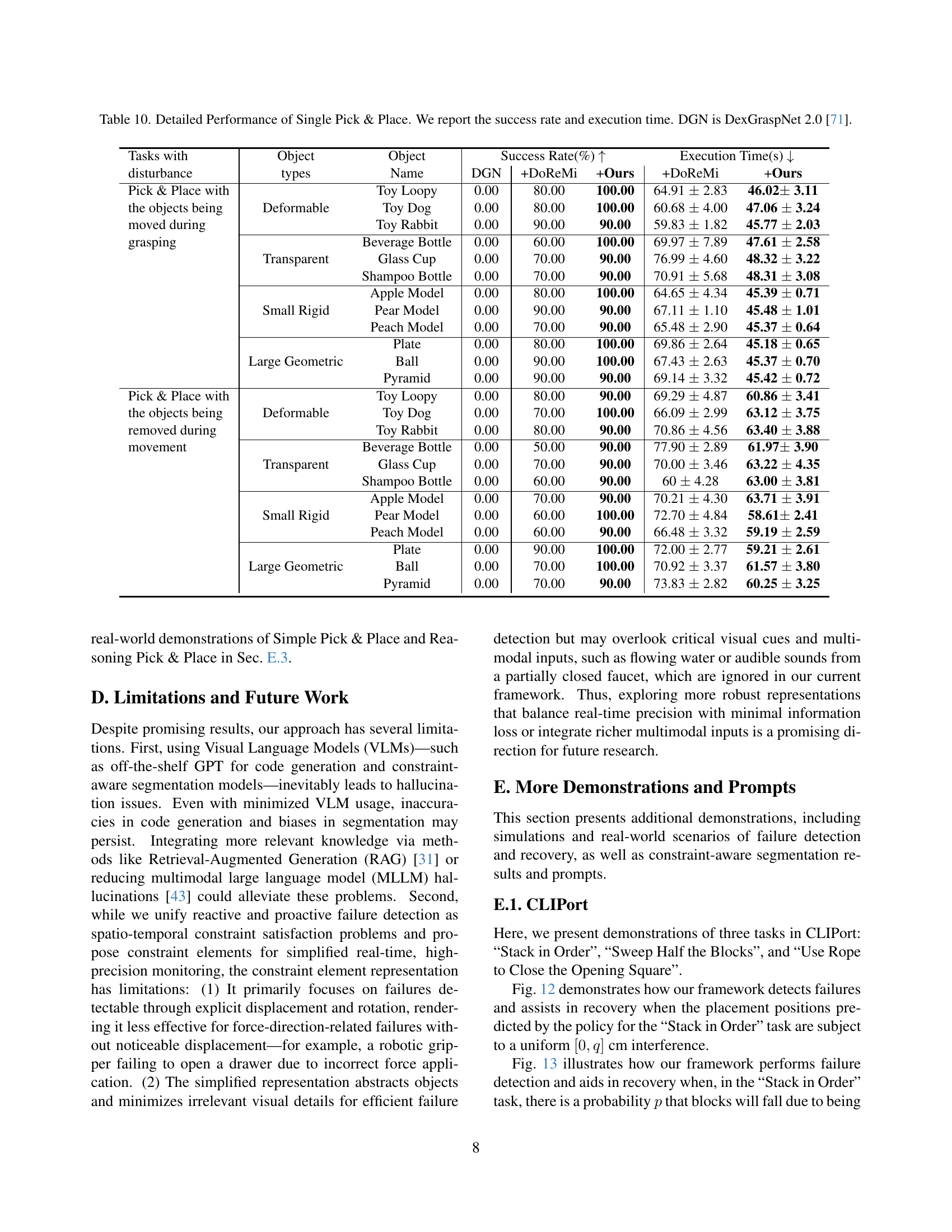
🔼 This table presents the success rate and execution time of a single pick-and-place task in a real-world setting. The task involves picking and placing objects of various types (deformable, transparent, small rigid, and large geometric) using a robot arm equipped with a dexterous hand. DexGraspNet 2.0 [71] is used as the low-level control policy. The results are broken down by object type and whether disturbances (moving the object during grasping, or removing the object from the hand during movement) were present.
read the caption
Table 3: Performance of Single Pick & Place. We report the success rate and execution time. DGN donates DexGraspNet 2.0 [71].
| Tasks | w/ CE | DGN | +DRM | +Ours |
|---|---|---|---|---|
| Clear all objects on table except for animals | ✓ | 0.00 | 10.00 | 60.00 |
| ✗ | 0.00 | 10.00 | 20.00 | |
| Grasp the animals according to their distances to fruits, from nearest to farthest | ✓ | 0.00 | 0.00 | 90.00 |
🔼 This table presents the success rates of a reasoning pick-and-place task in a cluttered scene. The experiment uses the DexGraspNet 2.0 (DGN) open-loop control policy. Two conditions are compared: one where constraint elements are used for tracking and code generation, and another where constraint-aware entities or parts are used instead. The results show the impact of using constraint elements on task success.
read the caption
Table 4: Performance of Reasoning Pick & Place in cluttered scene. We report the success rate. The robot is controlled by an open-loop policy named DexGraspNet 2.0 (DGN) [71]. w/ CE with ✓✓\checkmark✓ indicates using constraint elements; otherwise, constraint-aware entities or parts are used for tracking and code computation.
| Method | ReasonSeg Instance-level | ConstraintSeg Instance-level | Part-level | |||
|---|---|---|---|---|---|---|
| gIoU | cIoU | gIoU | cIoU | gIoU | cIoU | |
| OVSeg [35] | 28.5 | 18.6 | 32.9 | 31.4 | 20.2 | 21.5 |
| GRES [37] | 22.4 | 19.9 | 28.6 | 26.4 | 22.7 | 22.6 |
| X-Decoder [78] | 22.6 | 17.9 | 27.8 | 28.0 | 23.5 | 25.1 |
| SEEM [79] | 25.5 | 21.2 | 29.4 | 28.0 | 23.1 | 24.8 |
| PixelLM [52] | 56.0 | 61.4 | 44.4 | 43.2 | 24.1 | 22.6 |
| LISA-13B [28] | 56.6 | 65.1 | 42.1 | 38.9 | 23.4 | 24.3 |
| FMC | 51.2 | 53.3 | 49.3 | 49.6 | 40.8 | 39.3 |
| ConSeg-13B | 55.7 | 63.9 | 62.1 | 68.7 | 60.2 | 65.3 |
🔼 This table presents a comparison of the performance of different methods for reasoning and constraint-aware image segmentation. The methods compared include a foundation model combination baseline (FMC) and the proposed ConSeg model. The evaluation metrics used are likely IoU (Intersection over Union) and its various forms, assessing the accuracy of the segmentation results at both the instance and part levels.
read the caption
Table 5: Performance of reasoning and constraint-aware segmentation. FMC denotes the foundation model combination baseline.
| MV | CS | CP | None | Dist.(a) | Dist.(b) | Dist.(c) | Avg | |
|---|---|---|---|---|---|---|---|---|
| ✗ | ✓ | ✓ | 40.0 | 40.0 | 30.0 | 50.0 | 40.0 | |
| ✓ | ✗ | ✓ | 50.0 | 40.0 | 40.0 | 40.0 | 42.5 | |
| ✓ | ✓ | ✗ | 60.0 | 50.0 | 60.0 | 50.0 | 55.0 | |
| ✓ | ✓ | ✓ | 70.0 | 60.0 | 70.0 | 60.0 | 65.0 |
🔼 This table presents the results of ablation studies conducted on the ‘Stow Book’ task within the Omnigibson simulator. The study investigates the individual and combined effects of three key components of the Code-as-Monitor framework: Multi-View (MV) processing, Constraint-aware Segmentation (CS) for generating constraint elements, and the Connect Points (CP) algorithm used for creating constraint elements. The table shows how the success rate of the task varies depending on the presence or absence of each component, providing insights into their relative contributions to overall performance.
read the caption
Table 6: Ablation studies in Omnigibson’s “Stow Book”, assessing the impact of Multi-View (MV), Constraint-aware Segmentation (CS) for elements, and Connect Points (CP) for element formation.
| SemanticSeg | ReferSeg | VQA | ReasonSeg | ConstraintSeg | Ins-level | Part-level | |||
|---|---|---|---|---|---|---|---|---|---|
| Ins | Part | gIoU | cIoU | gIoU | cIoU | ||||
| ✓ | ✓ | ✓ | ✓ | ✗ | ✗ | 42.1 | 38.9 | 23.4 | 24.3 |
| ✓ | ✓ | ✓ | ✓ | ✓ | ✗ | 60.7 | 65.9 | 40.4 | 45.6 |
| ✓ | ✓ | ✓ | ✓ | ✗ | ✓ | 51.5 | 50.6 | 56.5 | 61.7 |
| ✓ | ✓ | ✓ | ✓ | ✓ | ✓ | 62.1 | 68.7 | 60.2 | 65.3 |
🔼 This table presents the results of an ablation study investigating the impact of different training data components on the performance of the constraint-aware segmentation model, ConSeg. The study specifically examines the contribution of instance-level and part-level segmentation data, along with the inclusion of various datasets for semantic segmentation (SemanticSeg), referring expression segmentation (ReferSeg), and visual question answering (VQA). The goal is to determine which data sources are most crucial for achieving high performance in ConSeg.
read the caption
Table 7: Ablation study on training data. SemanticSeg includes ADE20K [76], COCO-Stuff [5], PACO-LVIS [50] and PASCAL-Part [6]. ReferSeg includes refCLEF, refCOCO, refCOCO+ [26] and refCOCOg [42]. VQA indicates LLaVAInstruct-150k [39].
| Tasks with | Success Rate(%) ↑ | Execution Time(s) ↓ |
|---|---|---|
| disturbance | CLIPort | +Inner Monologue |
| Stack in p=0.0 | p=0.0 | 100.00 ± 0.00 |
| order with p=0.15 | p=0.15 | 56.67 ± 6.11 |
| drop p | p=0.3 | 21.67 ± 8.33 |
| Stack in q=1 | q=1 | 90.00 ± 6.11 |
| order with q=2 | q=2 | 41.67 ± 7.30 |
| noise q | q=3 | 15.00 ± 6.11 |
| Sweep Half the Blocks | 0.00 ± 0.00 | |
| Use Rope to Close the Opening Square | 0.00 ± 0.00 |
🔼 This table presents a detailed comparison of the performance of four different methods on three robotic manipulation tasks within the CLIPort simulator. The methods compared are the original CLIPort method, CLIPort enhanced with Inner Monologue, CLIPort with DoReMi, and the proposed Code-as-Monitor (CaM) method. For each task and method, the table reports the success rate (percentage of successful task completions) and the average execution time (in seconds) required to complete the task. The tasks include stacking blocks in a specific order (with variations in the probability of blocks dropping and noise in placement positions), sweeping half of a set of blocks into a designated area, and using a rope to enclose an open square. The results allow for a quantitative assessment of CaM’s performance against established baselines, highlighting its improvements in terms of both success rate and efficiency.
read the caption
Table 8: Detailed Performance in CLIPort. We report the success rate and execution time for three tasks, compared to baseline methods.
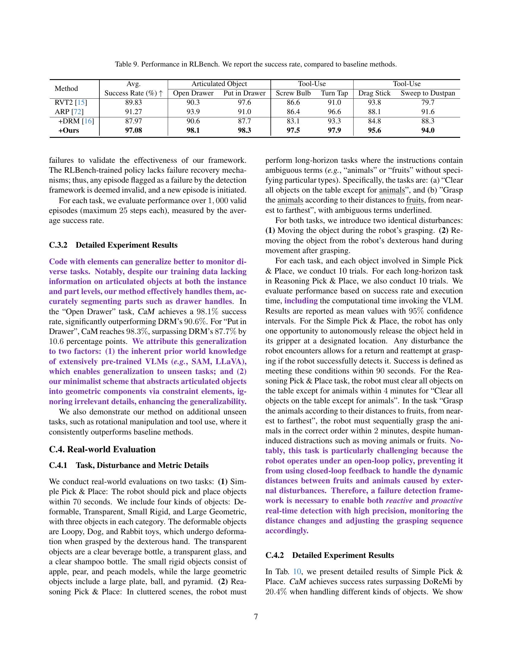
| Method | Avg. Success Rate (%) ↑ | Articulated Object Open Drawer | Articulated Object Put in Drawer | Tool-Use Screw Bulb | Tool-Use Turn Tap | Tool-Use Drag Stick | Tool-Use Sweep to Dustpan |
|---|---|---|---|---|---|---|---|
| RVT2 [15] | 89.83 | 90.3 | 97.6 | 86.6 | 91.0 | 93.8 | 79.7 |
| ARP [72] | 91.27 | 93.9 | 91.0 | 86.4 | 96.6 | 88.1 | 91.6 |
| +DRM [16] | 87.97 | 90.6 | 87.7 | 83.1 | 93.3 | 84.8 | 88.3 |
| +Ours | 97.08 | 98.1 | 98.3 | 97.5 | 97.9 | 95.6 | 94.0 |
🔼 This table presents a comparison of success rates achieved by different methods on various tasks within the RLBench environment. The methods include two baseline methods, DoReMi and the original RLBench method, and the proposed ‘Code-as-Monitor’ approach. The tasks are categorized into articulated object interaction, rotational manipulation, and tool use, offering a comprehensive evaluation across diverse robotic manipulation scenarios.
read the caption
Table 9: Performance in RLBench. We report the success rate, compared to baseline methods.
🔼 This table presents a detailed breakdown of the success rates and execution times for a single pick-and-place task across various object types, using DexGraspNet 2.0 [71] as a baseline method. The object types are categorized as deformable, transparent, small rigid, and large geometric. For each object type, the table shows the success rate and execution time for two scenarios: (1) objects are moved while being grasped, and (2) objects are removed from the robot hand during movement. This allows for a comprehensive analysis of the performance differences across various object types and disturbance conditions.
read the caption
Table 10: Detailed Performance of Single Pick & Place. We report the success rate and execution time. DGN is DexGraspNet 2.0 [71].
Full paper#
