↗ arXiv ↗ Hugging Face ↗ Papers with Code
TL;DR#
Many machine learning methods for solving partial differential equations (PDEs) struggle with accuracy, especially when dealing with high-frequency or non-linear components of the solution. These methods often rely on fixed grid representations or neural networks with inherent limitations. The challenge lies in efficiently allocating computational resources to capture complex features of the solution without overfitting. Existing techniques frequently require very high-resolution grids or a large number of collocation points which are computationally expensive and may lead to overfitting.
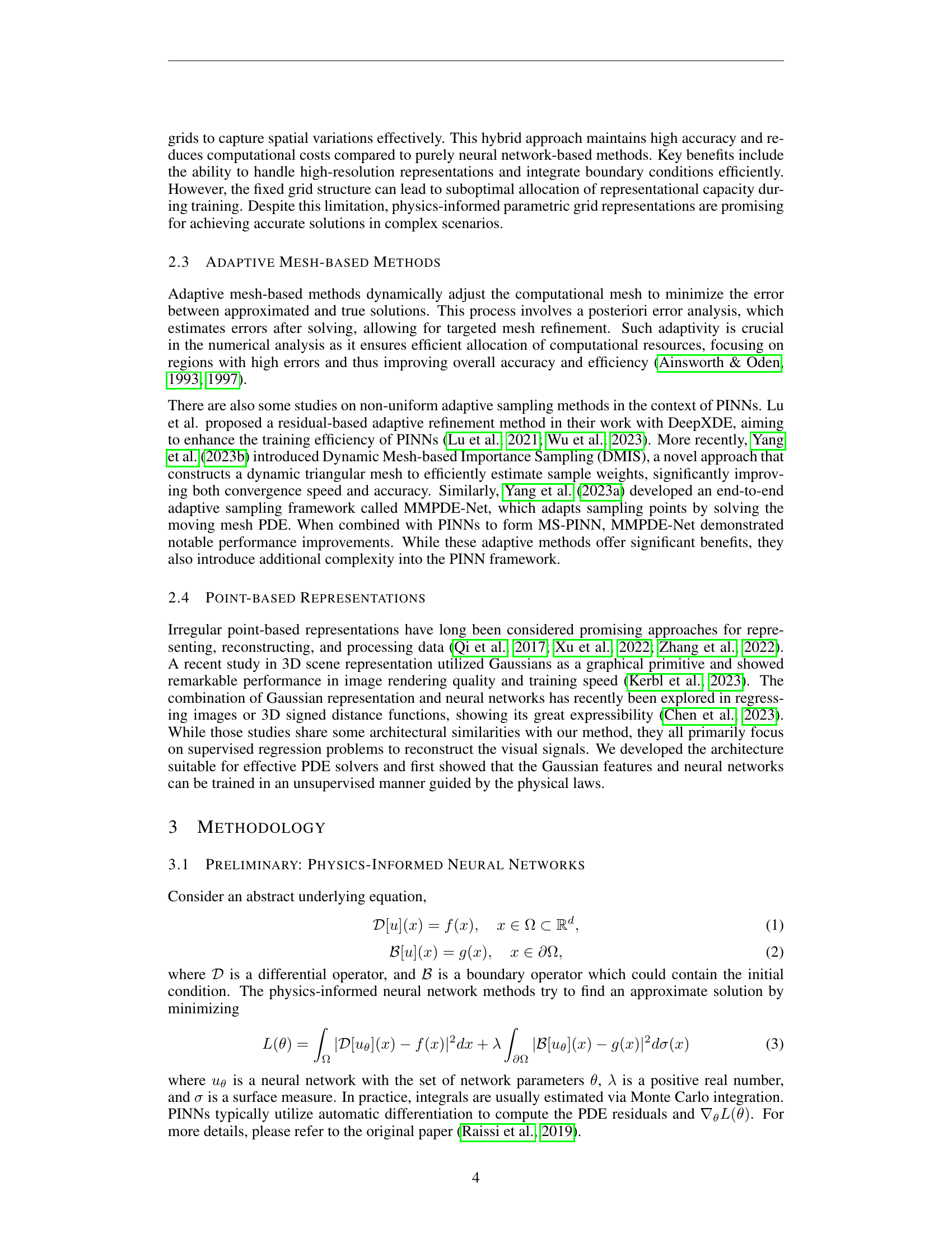
Physics-Informed Gaussians (PIGs) offer a novel approach. Instead of fixed grid points, PIGs use trainable Gaussian functions. The mean and variance of each Gaussian are learned during training, allowing the model to dynamically adjust the location and shape of these functions to focus on areas with high variations in the solution. This adaptive mesh representation effectively addresses the limitations of existing methods, resulting in improved accuracy and faster convergence. Experimental results demonstrate PIGs’ competitive performance and efficiency across diverse PDEs.
Key Takeaways#
Why does it matter?#
This paper is crucial for researchers working on solving partial differential equations (PDEs) using machine learning. It introduces a novel method that significantly improves accuracy and efficiency compared to existing techniques. The adaptive nature of the approach, using learnable Gaussian functions, allows for better approximation of complex PDEs, especially those with high-frequency components and singularities. This work also opens new avenues for research in adaptive mesh refinement and the integration of machine learning techniques with numerical methods for PDEs, making it highly relevant to current trends.
Visual Insights#

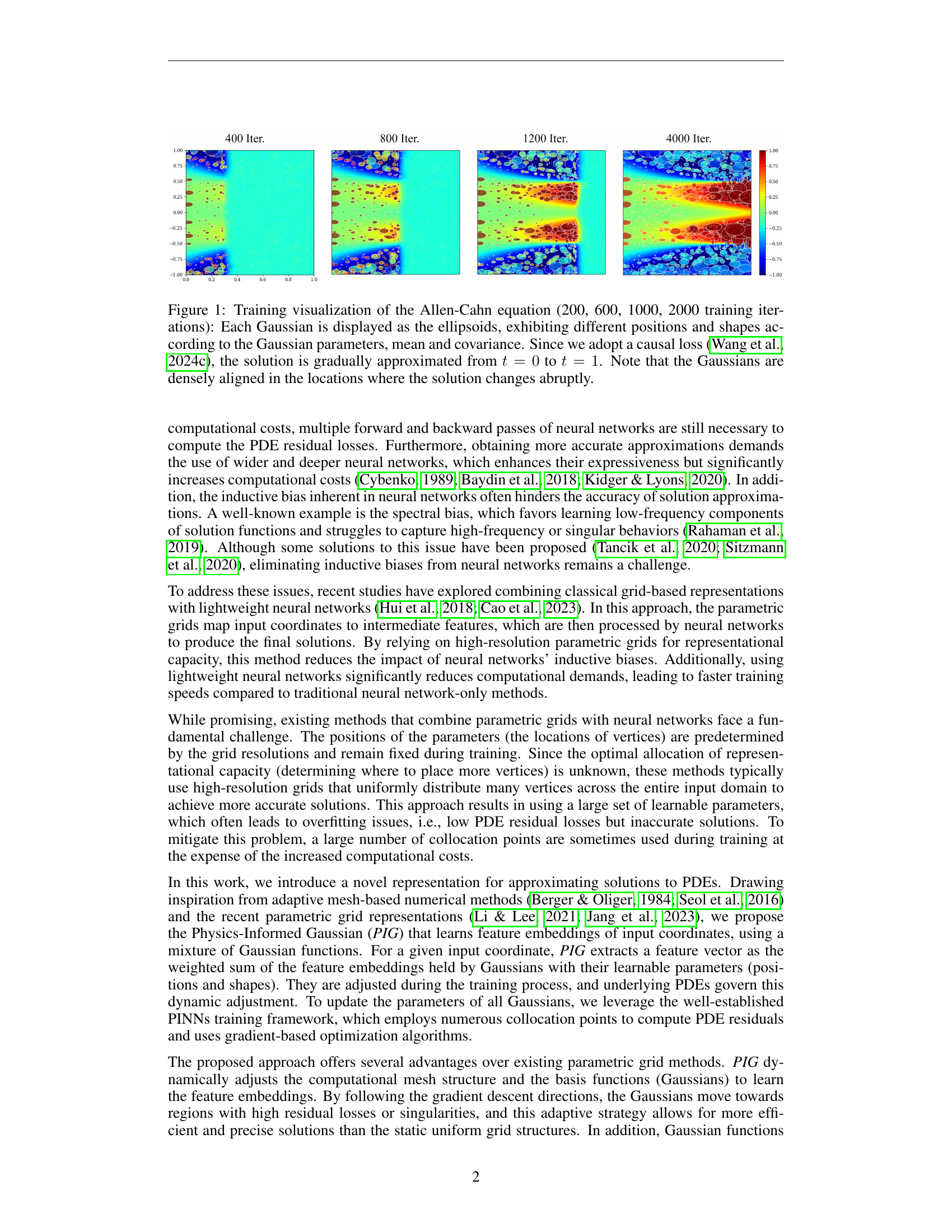
🔼 Figure 1 visualizes the training process of a Physics-Informed Gaussian (PIG) model solving the Allen-Cahn equation. The figure displays snapshots at 200, 600, 1000, and 2000 training iterations. Each ellipsoid represents a Gaussian function within the PIG model, and their size, shape, and position dynamically adapt during training based on their learned mean and covariance parameters. The color within each ellipsoid indicates the weight of the Gaussian at that position. The use of a causal loss function ensures the solution is progressively learned from time t=0 to t=1. Noticeably, the Gaussian functions tend to cluster and become more numerous in areas where the solution changes rapidly, demonstrating the adaptive nature of the PIG model.
read the caption
Figure 1: Training visualization of the Allen-Cahn equation (200, 600, 1000, 2000 training iterations): Each Gaussian is displayed as the ellipsoids, exhibiting different positions and shapes according to the Gaussian parameters, mean and covariance. Since we adopt a causal loss (Wang et al., 2024c), the solution is gradually approximated from t=0𝑡0t=0italic_t = 0 to t=1𝑡1t=1italic_t = 1. Note that the Gaussians are densely aligned in the locations where the solution changes abruptly.
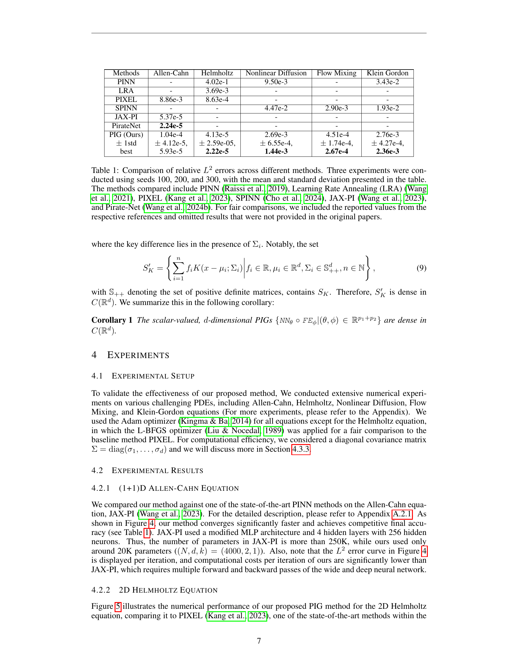
| Methods | Allen-Cahn | Helmholtz | Nonlinear Diffusion | Flow Mixing | Klein Gordon |
|---|---|---|---|---|---|
| PINN | - | 4.02e-1 | 9.50e-3 | - | 3.43e-2 |
| LRA | - | 3.69e-3 | - | - | - |
| PIXEL | 8.86e-3 | 8.63e-4 | - | - | - |
| SPINN | - | - | 4.47e-2 | 2.90e-3 | 1.93e-2 |
| JAX-PI | 5.37e-5 | - | - | - | - |
| PirateNet | 2.24e-5 | - | - | - | - |
| PIG (Ours) | 1.04e-4 | 4.13e-5 | 2.69e-3 | 4.51e-4 | 2.76e-3 |
| ± 1std | ± 4.12e-5 | ± 2.59e-05 | ± 6.55e-4 | ± 1.74e-4 | ± 4.27e-4 |
| best | 5.93e-5 | 2.22e-5 | 1.44e-3 | 2.67e-4 | 2.36e-3 |
🔼 This table compares the performance of various methods for approximating solutions to partial differential equations (PDEs) by showing their relative L2 errors. The comparison includes several state-of-the-art methods like PINN, Learning Rate Annealing (LRA), PIXEL, SPINN, JAX-PI, and Pirate-Net. The results are averaged over three separate experiments with different random seeds (100, 200, 300) to assess the robustness of the methods. Mean and standard deviation of L2 errors are presented for a comprehensive evaluation. Note that for fair comparisons, only results reported in the original papers for each method are included.
read the caption
Table 1: Comparison of relative L2superscript𝐿2L^{2}italic_L start_POSTSUPERSCRIPT 2 end_POSTSUPERSCRIPT errors across different methods. Three experiments were conducted using seeds 100, 200, and 300, with the mean and standard deviation presented in the table. The methods compared include PINN (Raissi et al., 2019), Learning Rate Annealing (LRA) (Wang et al., 2021), PIXEL (Kang et al., 2023), SPINN (Cho et al., 2024), JAX-PI (Wang et al., 2023), and Pirate-Net (Wang et al., 2024b). For fair comparisons, we included the reported values from the respective references and omitted results that were not provided in the original papers.
In-depth insights#
Physics-Informed Gaussian#
The concept of “Physics-Informed Gaussians” presents a novel approach to solving partial differential equations (PDEs) by combining the strengths of Gaussian processes and physics-informed neural networks (PINNs). The core idea involves using trainable Gaussian functions as basis functions to represent the solution space. Instead of fixed grid points like in traditional finite element methods or even parametric grid methods, the Gaussians’ means and covariances are learned during training, allowing for adaptive mesh refinement. This adaptability is crucial, as it enables the model to focus computational resources on areas where the solution is most complex or changes rapidly, leading to improved efficiency and accuracy. The integration with PINNs maintains the straightforward optimization framework, leveraging gradient-based methods for training. The use of Gaussians, with their smooth, infinitely differentiable nature, offers benefits in gradient computation for PDE residuals. By dynamically adjusting positions and shapes of the Gaussians, the method aims to overcome spectral bias issues commonly seen in standard neural networks applied to PDEs. Overall, Physics-Informed Gaussians offer a promising alternative that blends the advantages of mesh-free learning with adaptive mesh capabilities for superior performance in solving complex PDEs.
Adaptive Meshing#
Adaptive meshing, in the context of solving partial differential equations (PDEs), is a crucial technique for optimizing computational efficiency and solution accuracy. Traditional methods often employ uniform grids, which can be computationally expensive and inefficient, especially when dealing with complex geometries or solutions exhibiting high gradients in localized areas. Adaptive meshing dynamically refines the mesh resolution in regions requiring higher accuracy, such as near boundaries or discontinuities, while coarsening the mesh in areas with smoother solutions. This approach ensures that computational resources are concentrated where they are most needed, leading to significant reductions in computational cost without sacrificing accuracy. Several strategies exist for implementing adaptive meshing, including error-based refinement, where the mesh is refined based on estimated errors in the solution, and feature-based refinement, which focuses on resolving features of interest. The choice of adaptive meshing strategy depends on the specific problem, the available computational resources, and the desired level of accuracy. For PDEs solved by neural networks, adaptive meshing is a particularly valuable tool for handling complex solutions efficiently. The optimal mesh density is not known in advance, and it evolves throughout training. This necessitates adaptive mechanisms that dynamically allocate computational resources throughout training.
UAT for PIGs#
The Universal Approximation Theorem (UAT) for Physics-Informed Gaussians (PIGs) is a crucial aspect of the research paper. A rigorous proof of the UAT for PIGs would formally establish the capability of the model to approximate any continuous function, a fundamental property for a successful PDE solver. The proof likely focuses on the expressive power of the Gaussian feature embedding and lightweight neural network components of the PIG architecture. It would address how the combination of trainable Gaussian parameters (means and covariances) and the neural network enables the representation of complex functions. The interplay between the localized nature of Gaussian functions and the global approximation capacity of the neural network is a key element of this analysis. It is important to understand how the model’s adaptability, through the dynamic adjustment of Gaussian positions, interacts with the theoretical guarantees of approximation provided by the UAT. The UAT for PIGs, thus, connects the model’s architecture with its functional capabilities, supporting the claim of robustness and efficiency across a range of PDEs.
Empirical Validation#
An ‘Empirical Validation’ section in a PDF research paper is crucial for demonstrating the practical effectiveness of the proposed methods. It should present rigorous experiments on diverse and challenging datasets, carefully designed to test the model’s capabilities and limitations. The section needs to detail the experimental setup, including dataset characteristics, evaluation metrics, and parameter choices. Comparative analysis against existing state-of-the-art approaches is vital to establish the novelty and superiority of the proposed method. Results should be clearly presented through tables, figures, and statistical analysis, highlighting both the strengths and weaknesses of the method. Error analysis, including different types of errors, and an investigation into factors impacting performance, such as hyperparameter tuning, should also be included. A thoughtful discussion of the results, relating them back to the theoretical foundations of the paper, is necessary to provide a comprehensive and insightful validation of the research claims. Ultimately, a strong ‘Empirical Validation’ section builds confidence in the scientific rigor and practical impact of the research.
Future Research#
Future research directions stemming from this PDF could involve exploring more sophisticated adaptive mechanisms for the Gaussian parameters. The current approach dynamically adjusts parameters, but more intelligent strategies, potentially incorporating reinforcement learning or advanced optimization techniques, could yield substantial improvements in accuracy and efficiency. Another avenue would be to investigate alternative basis functions beyond Gaussians, perhaps exploring combinations of different functions to better capture diverse solution behaviors. The current framework uses a relatively simple neural network; incorporating more complex architectures, such as convolutional or recurrent networks, might further enhance the model’s ability to approximate complex PDEs. Finally, a crucial area for future work is rigorous theoretical analysis. Establishing convergence guarantees and a deeper understanding of the model’s limitations could greatly improve its practical usability and lead to the development of more robust and reliable PDE solvers. The application to higher-dimensional problems could also benefit from exploring advanced numerical techniques to manage computational costs.
More visual insights#
More on figures

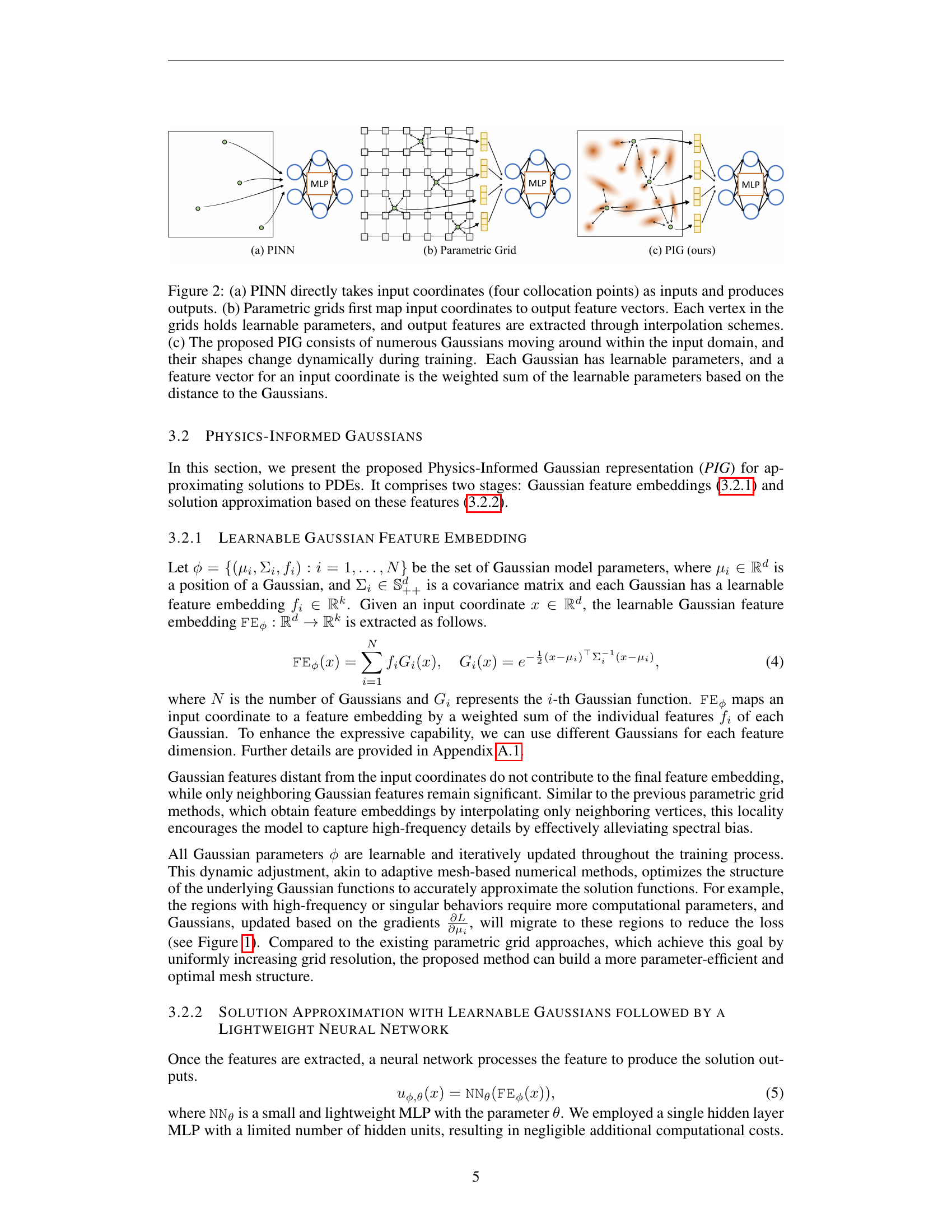
🔼 Figure 2 illustrates the architectures of three different PDE solving methods: (a) PINN, (b) Parametric Grid, and (c) PIG (Physics-Informed Gaussian). In (a), a PINN directly uses input coordinates as input and generates output values through a neural network. (b) shows a parametric grid method where input coordinates are mapped to feature vectors. The vertices of this grid contain learnable parameters, which are interpolated to produce the final output. Finally, (c) displays the proposed PIG approach. Multiple Gaussian functions, each with learnable parameters (mean, covariance, and feature embedding), dynamically adapt their position and shape during training. The final feature vector for a given coordinate is a weighted sum of these Gaussian functions, with the weights determined by proximity to the input coordinate. This dynamic adjustment allows PIG to efficiently focus its computational resources on areas where the solution changes significantly.
read the caption
Figure 2: (a) PINN directly takes input coordinates (four collocation points) as inputs and produces outputs. (b) Parametric grids first map input coordinates to output feature vectors. Each vertex in the grids holds learnable parameters, and output features are extracted through interpolation schemes. (c) The proposed PIG consists of numerous Gaussians moving around within the input domain, and their shapes change dynamically during training. Each Gaussian has learnable parameters, and a feature vector for an input coordinate is the weighted sum of the learnable parameters based on the distance to the Gaussians.

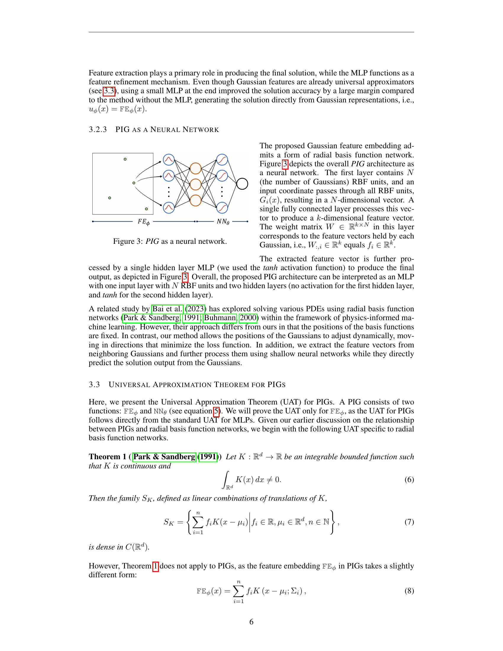
🔼 This figure illustrates the architecture of the Physics-Informed Gaussian (PIG) model as a neural network. The input is a coordinate, which is passed through a layer of radial basis functions (RBFs), one for each Gaussian in the model. Each RBF produces a weighted contribution based on the distance from the coordinate to the Gaussian’s center. These weighted contributions are then combined to form a feature vector. This feature vector is fed into a multilayer perceptron (MLP), which refines the features and produces the final output, which is the solution to the PDE. The weights of the Gaussian feature embeddings are learnable, as are the weights of the MLP.
read the caption
Figure 3: PIG as a neural network.

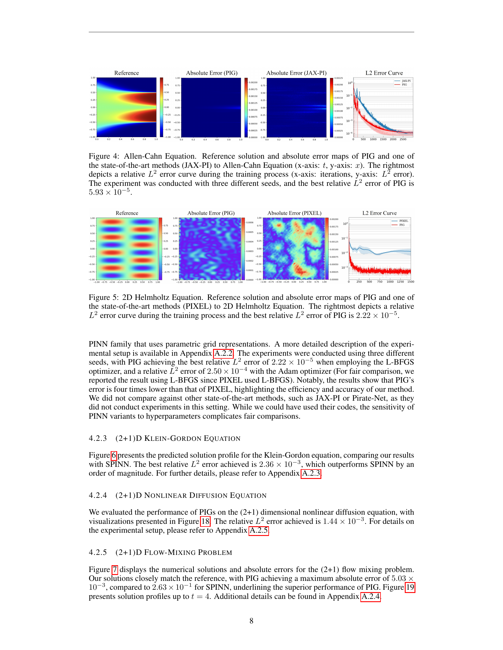
🔼 Figure 4 presents a comparison of the Allen-Cahn equation’s solution and error maps generated by PIG and JAX-PI. The left panels show the reference solution and the absolute error maps for both methods. The x-axis represents the spatial dimension (x), and the y-axis represents the time dimension (t). The right panel displays the L2 error curves during training for both methods, illustrating convergence over training iterations. The best relative L2 error achieved by PIG is 5.93 x 10^-5.
read the caption
Figure 4: Allen-Cahn Equation. Reference solution and absolute error maps of PIG and one of the state-of-the-art methods (JAX-PI) to Allen-Cahn Equation (x-axis: t𝑡titalic_t, y-axis: x𝑥xitalic_x). The rightmost depicts a relative L2superscript𝐿2L^{2}italic_L start_POSTSUPERSCRIPT 2 end_POSTSUPERSCRIPT error curve during the training process (x-axis: iterations, y-axis: L2superscript𝐿2L^{2}italic_L start_POSTSUPERSCRIPT 2 end_POSTSUPERSCRIPT error). The experiment was conducted with three different seeds, and the best relative L2superscript𝐿2L^{2}italic_L start_POSTSUPERSCRIPT 2 end_POSTSUPERSCRIPT error of PIG is 5.93×10−55.93superscript1055.93\times 10^{-5}5.93 × 10 start_POSTSUPERSCRIPT - 5 end_POSTSUPERSCRIPT.

🔼 Figure 5 presents a comparison of the proposed Physics-Informed Gaussian (PIG) model and the PIXEL method for solving the 2D Helmholtz equation. It showcases the reference solution alongside absolute error maps generated by both PIG and PIXEL. This visual comparison highlights the accuracy of each method in approximating the solution. The graph on the right displays the relative L2 error over the training iterations, demonstrating PIG’s superior performance with a best relative L2 error of 2.22 x 10^-5.
read the caption
Figure 5: 2D Helmholtz Equation. Reference solution and absolute error maps of PIG and one of the state-of-the-art methods (PIXEL) to 2D Helmholtz Equation. The rightmost depicts a relative L2superscript𝐿2L^{2}italic_L start_POSTSUPERSCRIPT 2 end_POSTSUPERSCRIPT error curve during the training process and the best relative L2superscript𝐿2L^{2}italic_L start_POSTSUPERSCRIPT 2 end_POSTSUPERSCRIPT error of PIG is 2.22×10−52.22superscript1052.22\times 10^{-5}2.22 × 10 start_POSTSUPERSCRIPT - 5 end_POSTSUPERSCRIPT.

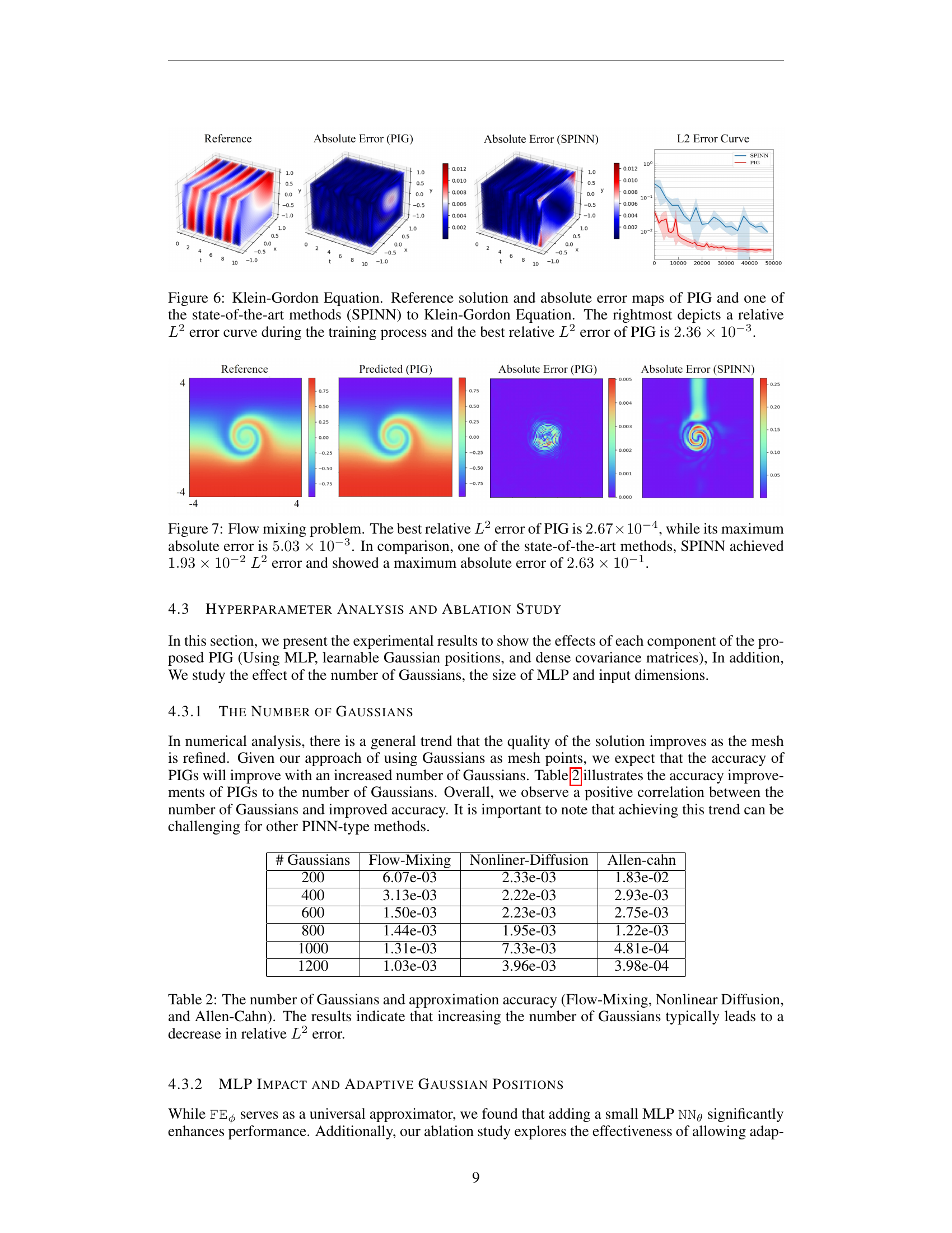
🔼 Figure 6 presents a comparison of the performance of the Physics-Informed Gaussian (PIG) model and the state-of-the-art SPINN model on the Klein-Gordon equation. The figure displays three subplots. The left subplot shows the reference solution, the center shows the absolute error for the PIG model, and the subplot on the right displays the absolute error of SPINN. The rightmost subplot is a graph showing the relative L2 error over the course of training for both models, illustrating that the PIG model achieves a lower relative L2 error (2.36e-3) than SPINN.
read the caption
Figure 6: Klein-Gordon Equation. Reference solution and absolute error maps of PIG and one of the state-of-the-art methods (SPINN) to Klein-Gordon Equation. The rightmost depicts a relative L2superscript𝐿2L^{2}italic_L start_POSTSUPERSCRIPT 2 end_POSTSUPERSCRIPT error curve during the training process and the best relative L2superscript𝐿2L^{2}italic_L start_POSTSUPERSCRIPT 2 end_POSTSUPERSCRIPT error of PIG is 2.36×10−32.36superscript1032.36\times 10^{-3}2.36 × 10 start_POSTSUPERSCRIPT - 3 end_POSTSUPERSCRIPT.

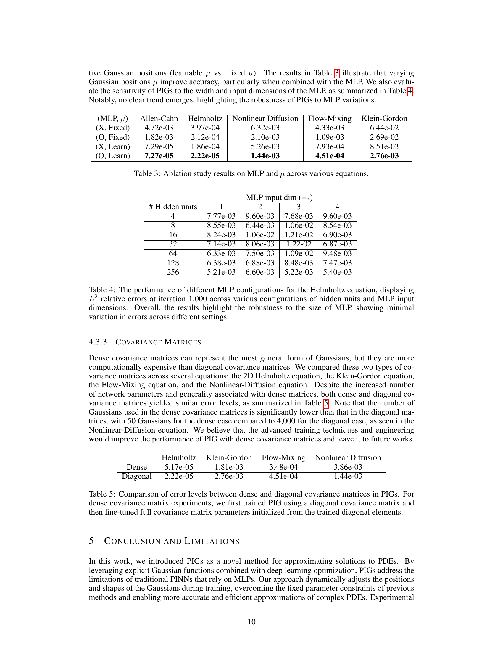
🔼 Figure 7 presents a comparison of the Flow Mixing problem results obtained using Physics-Informed Gaussian (PIG) and state-of-the-art SPINN methods. The visualizations show the reference solution, the PIG’s prediction, and the absolute error. PIG demonstrates significantly improved accuracy, achieving a best relative L2 error of 2.67 x 10⁻⁴ and a maximum absolute error of 5.03 x 10⁻³. This is a substantial improvement over SPINN, which achieved a relative L2 error of 1.93 x 10⁻² and a maximum absolute error of 2.63 x 10⁻¹.
read the caption
Figure 7: Flow mixing problem. The best relative L2superscript𝐿2L^{2}italic_L start_POSTSUPERSCRIPT 2 end_POSTSUPERSCRIPT error of PIG is 2.67×10−42.67superscript1042.67\times 10^{-4}2.67 × 10 start_POSTSUPERSCRIPT - 4 end_POSTSUPERSCRIPT, while its maximum absolute error is 5.03×10−35.03superscript1035.03\times 10^{-3}5.03 × 10 start_POSTSUPERSCRIPT - 3 end_POSTSUPERSCRIPT. In comparison, one of the state-of-the-art methods, SPINN achieved 1.93×10−21.93superscript1021.93\times 10^{-2}1.93 × 10 start_POSTSUPERSCRIPT - 2 end_POSTSUPERSCRIPT L2superscript𝐿2L^{2}italic_L start_POSTSUPERSCRIPT 2 end_POSTSUPERSCRIPT error and showed a maximum absolute error of 2.63×10−12.63superscript1012.63\times 10^{-1}2.63 × 10 start_POSTSUPERSCRIPT - 1 end_POSTSUPERSCRIPT.

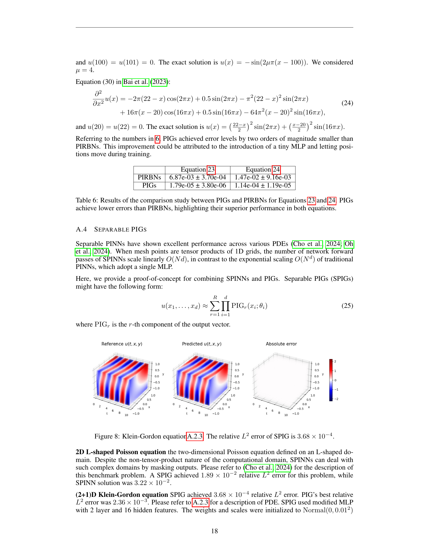
🔼 Figure 8 displays the results of applying the Separable Physics-Informed Gaussian (SPIG) method to the (2+1)D Klein-Gordon equation. The figure visually compares the reference solution (exact solution) against the solution predicted by the SPIG model, showing the absolute error. The relative L2 error achieved by the SPIG method for this problem is 3.68 x 10^-4, which indicates a high level of accuracy in approximating the solution.
read the caption
Figure 8: Klein-Gordon equationA.2.3. The relative L2superscript𝐿2L^{2}italic_L start_POSTSUPERSCRIPT 2 end_POSTSUPERSCRIPT error of SPIG is 3.68×10−43.68superscript1043.68\times 10^{-4}3.68 × 10 start_POSTSUPERSCRIPT - 4 end_POSTSUPERSCRIPT.

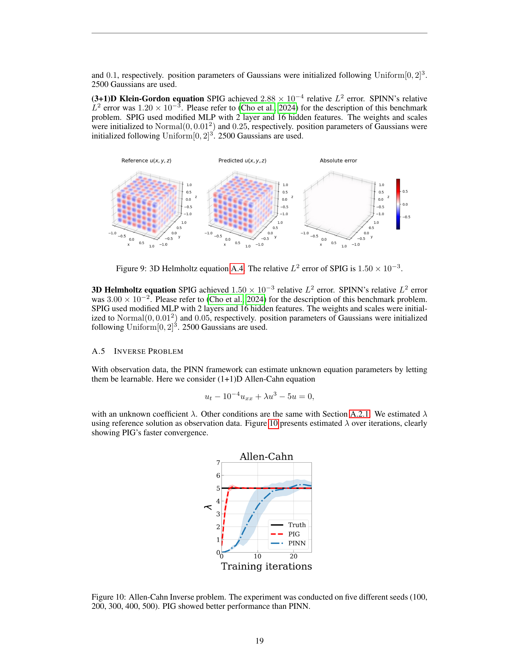
🔼 Figure 9 presents the results of applying the Separable Physics-Informed Gaussian (SPIG) method to solve a 3D Helmholtz equation. The figure shows that SPIG achieves a relative L2 error of 1.50 x 10^-3. This demonstrates the accuracy of SPIG in handling high-dimensional problems, especially when compared to the results obtained using other methods described in the paper.
read the caption
Figure 9: 3D Helmholtz equation 9. The relative L2superscript𝐿2L^{2}italic_L start_POSTSUPERSCRIPT 2 end_POSTSUPERSCRIPT error of SPIG is 1.50×10−31.50superscript1031.50\times 10^{-3}1.50 × 10 start_POSTSUPERSCRIPT - 3 end_POSTSUPERSCRIPT.

🔼 Figure 10 presents a comparison of the performance of Physics-Informed Gaussians (PIG) and Physics-Informed Neural Networks (PINN) on an inverse problem for the Allen-Cahn equation. The Allen-Cahn equation is a partial differential equation modeling phase separation processes. In an inverse problem, the goal is to determine unknown parameters of the equation, such as a coefficient, based on observed data. The figure shows the estimated values of the unknown parameter (lambda) over training iterations for both methods. The experiment was repeated five times using different random seeds (100, 200, 300, 400, and 500) to assess the robustness and stability of the algorithms. PIG demonstrates faster convergence and achieves a more accurate estimate of the parameter than PINN. This highlights the effectiveness of PIGs in solving inverse problems.
read the caption
Figure 10: Allen-Cahn Inverse problem. The experiment was conducted on five different seeds (100, 200, 300, 400, 500). PIG showed better performance than PINN.

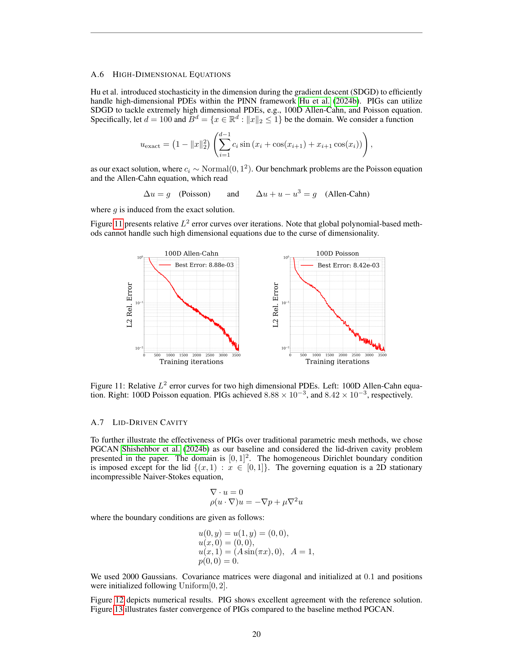
🔼 This figure displays the relative L2 error curves for 100-dimensional Allen-Cahn and Poisson equations, demonstrating the performance of Physics-Informed Gaussians (PIGs) in high-dimensional settings. The left panel shows the error curve for the Allen-Cahn equation, while the right panel displays the error curve for the Poisson equation. PIGs achieved a relative L2 error of 8.88 x 10^-3 for the Allen-Cahn equation and 8.42 x 10^-3 for the Poisson equation. These results showcase PIG’s ability to handle high-dimensional partial differential equations effectively.
read the caption
Figure 11: Relative L2superscript𝐿2L^{2}italic_L start_POSTSUPERSCRIPT 2 end_POSTSUPERSCRIPT error curves for two high dimensional PDEs. Left: 100D Allen-Cahn equation. Right: 100D Poisson equation. PIGs achieved 8.88×10−38.88superscript1038.88\times 10^{-3}8.88 × 10 start_POSTSUPERSCRIPT - 3 end_POSTSUPERSCRIPT, and 8.42×10−38.42superscript1038.42\times 10^{-3}8.42 × 10 start_POSTSUPERSCRIPT - 3 end_POSTSUPERSCRIPT, respectively.

🔼 Figure 12 presents a comparison of the results obtained using Physics-Informed Gaussians (PIG) and Parametric Grids with Convolutional Neural Networks (PG-CNN) for simulating a 2D Lid-driven cavity flow. The visualization showcases the reference solution alongside predictions generated by both methods. The absolute errors for each method are also displayed, highlighting the superior accuracy of PIG. PIG demonstrates a significantly lower relative L2 error (4.04 x 10^-4) compared to PGCAN (1.22 x 10^-3), indicating its improved accuracy in approximating complex flow patterns within the cavity.
read the caption
Figure 12: Lid-driven cavity flow problem. PIG achieved 4.04×10−44.04superscript1044.04\times 10^{-4}4.04 × 10 start_POSTSUPERSCRIPT - 4 end_POSTSUPERSCRIPT relative L2superscript𝐿2L^{2}italic_L start_POSTSUPERSCRIPT 2 end_POSTSUPERSCRIPT error whereas the baseline parametric grid method PGCAN resulted in 1.22×10−31.22superscript1031.22\times 10^{-3}1.22 × 10 start_POSTSUPERSCRIPT - 3 end_POSTSUPERSCRIPT.

🔼 Figure 13 displays the relative L2 error over training iterations for the lid-driven cavity problem. The plot compares the performance of Physics-Informed Gaussians (PIG) against Physics-Guided Cell Networks (PGCAN), a method that utilizes parametric grids. The results demonstrate that PIG achieves significantly lower relative L2 error (4.04 x 10⁻⁴) than PGCAN (1.22 x 10⁻³), showcasing PIG’s superior performance and efficiency in solving this specific problem.
read the caption
Figure 13: Relative L2superscript𝐿2L^{2}italic_L start_POSTSUPERSCRIPT 2 end_POSTSUPERSCRIPT error curve of the lid-driven cavity problem. PIG achieved 4.04×10−44.04superscript1044.04\times 10^{-4}4.04 × 10 start_POSTSUPERSCRIPT - 4 end_POSTSUPERSCRIPT and PGCAN which used the parametric grid method achieved 1.22×10−31.22superscript1031.22\times 10^{-3}1.22 × 10 start_POSTSUPERSCRIPT - 3 end_POSTSUPERSCRIPT.

🔼 This figure demonstrates the ability of Physics-Informed Gaussians (PIG) to effectively approximate solutions to partial differential equations (PDEs), specifically a 2D Helmholtz equation with high-frequency components (wavenumbers a1=10 and a2=10). PIG achieves a significantly lower relative L2 error (7.09e-3) compared to the Parametric Fixed Grid method PIXEL (7.47e-2), highlighting PIG’s superior performance in handling high-frequency details. The figure visually showcases the inability of traditional Physics-Informed Neural Networks (PINNs) to converge on this challenging problem.
read the caption
Figure 14: 2D Helmholtz equation with a high wavenumber (a1,a2)=(10,10)subscript𝑎1subscript𝑎21010(a_{1},a_{2})=(10,10)( italic_a start_POSTSUBSCRIPT 1 end_POSTSUBSCRIPT , italic_a start_POSTSUBSCRIPT 2 end_POSTSUBSCRIPT ) = ( 10 , 10 ). PIG achieved a relative L2superscript𝐿2L^{2}italic_L start_POSTSUPERSCRIPT 2 end_POSTSUPERSCRIPT error of 7.09×10−37.09superscript1037.09\times 10^{-3}7.09 × 10 start_POSTSUPERSCRIPT - 3 end_POSTSUPERSCRIPT, while the parametric fixed grid method PIXEL reached a relative L2superscript𝐿2L^{2}italic_L start_POSTSUPERSCRIPT 2 end_POSTSUPERSCRIPT error of 7.47×10−27.47superscript1027.47\times 10^{-2}7.47 × 10 start_POSTSUPERSCRIPT - 2 end_POSTSUPERSCRIPT. PINN failed to converge.

🔼 Figure 15 presents histograms visualizing the distribution of Gaussian parameters used in the Physics-Informed Gaussian (PIG) model for two distinct partial differential equations (PDEs): the flow-mixing equation and the Klein-Gordon equation. The top row displays histograms representing the minimum distances between the centers of adjacent Gaussian functions for each PDE. A distance greater than zero signifies that no two Gaussians occupy the same location; in other words, there is no mode collapse. The bottom row shows histograms of the variances (a measure of the spread) of the Gaussian functions. The non-zero variance values indicate that each Gaussian function has a unique and non-degenerate representation, thus preventing them from collapsing into a single point.
read the caption
Figure 15: Histograms of the Gaussian parameters for the flow-mixing equation and the Klein-Gordon equation. The upper panels display histograms of the minimum distances between the Gaussian centers, where distances >0absent0>0> 0 indicate the absence of mode collapse. The lower panels show histograms of the Gaussian variances, highlighting the non-degeneracy of the Gaussians.

🔼 Figure 16 presents a comparison of the Physics-Informed Gaussian (PIG) model and the Physics-Informed Gaussian Splatting (PI-GS) model for approximating solutions of the (2+1)D Burgers’ equation. The left panels show the reference solution at time t=0 and t=1, respectively. The middle panels illustrate the solution predicted by the PIG model at the same time points, and the right panels show the absolute error between the PIG prediction and the reference solution. The results demonstrate that PIG achieves significantly higher accuracy than PI-GS (a relative L2 error of 7.68e-04 versus 1.62e-01) while also being more computationally efficient (0.28 seconds per iteration versus 1.5 seconds per iteration). This highlights PIG’s superior performance in approximating solutions to complex PDEs.
read the caption
Figure 16: Prediction results of PIG for the first example of the (2+1)D Burgers’ equation. PIG achieved a relative L2superscript𝐿2L^{2}italic_L start_POSTSUPERSCRIPT 2 end_POSTSUPERSCRIPT error of 7.68×10−47.68superscript1047.68\times 10^{-4}7.68 × 10 start_POSTSUPERSCRIPT - 4 end_POSTSUPERSCRIPT, with a computation time of 0.28 seconds per iteration. In contrast, PI-GS attained a relative L2superscript𝐿2L^{2}italic_L start_POSTSUPERSCRIPT 2 end_POSTSUPERSCRIPT error of 1.62×10−11.62superscript1011.62\times 10^{-1}1.62 × 10 start_POSTSUPERSCRIPT - 1 end_POSTSUPERSCRIPT, requiring 1.50 seconds per iteration.

🔼 Figure 17 presents a comparison of the performance of Physics-Informed Gaussians (PIG) and Physics-Informed Gaussian Splats (PI-GS) in approximating the solution of the (2+1)D Burgers’ equation. The initial condition for this example is a probability density function (PDF) representing a mixture of two Gaussian distributions. The figure showcases the reference solution at time t=0 and t=1, alongside the corresponding predictions generated by PIG and PI-GS. The results highlight PIG’s superior accuracy, achieving a relative L2 error of 1.08 x 10^-3 in only 0.29 seconds per iteration, compared to PI-GS’s relative L2 error of 2.61 x 10^-1, requiring significantly more computation time (1.68 seconds per iteration).
read the caption
Figure 17: Prediction results of PIG for the second example of the (2+1)D Burgers’ equation. PIG achieved a relative L2superscript𝐿2L^{2}italic_L start_POSTSUPERSCRIPT 2 end_POSTSUPERSCRIPT error of 1.08×10−31.08superscript1031.08\times 10^{-3}1.08 × 10 start_POSTSUPERSCRIPT - 3 end_POSTSUPERSCRIPT, with a computation time of 0.29 seconds per iteration. In comparison, PI-GS attained a relative L2superscript𝐿2L^{2}italic_L start_POSTSUPERSCRIPT 2 end_POSTSUPERSCRIPT error of 2.61×10−12.61superscript1012.61\times 10^{-1}2.61 × 10 start_POSTSUPERSCRIPT - 1 end_POSTSUPERSCRIPT, requiring 1.68 seconds per iteration.

🔼 Figure 18 presents the results of applying the Physics-Informed Gaussian (PIG) model to solve the 2D nonlinear diffusion equation (detailed in Section 4.2.4 of the paper). The figure visually compares the reference solution (the known, correct solution) with the solution predicted by the PIG model. It demonstrates the accuracy of the PIG model by showing how closely the predicted solution matches the reference solution. Three separate trials were conducted, using different random seeds (100, 200, and 300) to assess the model’s robustness and consistency. The caption indicates that the lowest relative L2 error achieved across these three trials was 1.44 x 10⁻³. This signifies a relatively small discrepancy between the model’s prediction and the actual solution.
read the caption
Figure 18: Non-linear diffusion equation 4.2.4. The experiment was conducted on three different seeds (100, 200, 300). The best relative L2superscript𝐿2L^{2}italic_L start_POSTSUPERSCRIPT 2 end_POSTSUPERSCRIPT error is 1.44×10−31.44superscript1031.44\times 10^{-3}1.44 × 10 start_POSTSUPERSCRIPT - 3 end_POSTSUPERSCRIPT.

🔼 Figure 19 presents the results of the flow mixing simulation at different time points (t=0, t=2, t=4). The simulation was run three times using different random seeds (100, 200, 300) to evaluate the reproducibility and stability of the model. The figure compares the exact analytical solution of the flow mixing equation with the solution predicted by the Physics-Informed Gaussian (PIG) model. The best relative L2 error achieved across these three runs was 2.67 x 10^-4. This demonstrates the accuracy of the PIG model in approximating the complex, time-dependent behavior of the flow mixing system.
read the caption
Figure 19: Flow mixing equation 4.2.5. The experiment was conducted on three different seeds (100, 200, 300). The best relative L2superscript𝐿2L^{2}italic_L start_POSTSUPERSCRIPT 2 end_POSTSUPERSCRIPT error is 2.67×10−42.67superscript1042.67\times 10^{-4}2.67 × 10 start_POSTSUPERSCRIPT - 4 end_POSTSUPERSCRIPT.
More on tables
| # Gaussians | Flow-Mixing | Nonliner-Diffusion | Allen-cahn |
|---|---|---|---|
| 200 | 6.07e-03 | 2.33e-03 | 1.83e-02 |
| 400 | 3.13e-03 | 2.22e-03 | 2.93e-03 |
| 600 | 1.50e-03 | 2.23e-03 | 2.75e-03 |
| 800 | 1.44e-03 | 1.95e-03 | 1.22e-03 |
| 1000 | 1.31e-03 | 7.33e-03 | 4.81e-04 |
| 1200 | 1.03e-03 | 3.96e-03 | 3.98e-04 |
🔼 This table presents the impact of varying the number of Gaussian functions on the accuracy of the Physics-Informed Gaussian (PIG) model in approximating solutions for three different partial differential equations (PDEs): Flow-Mixing, Nonlinear Diffusion, and Allen-Cahn. The relative L2 error, a common metric for assessing the accuracy of PDE solution approximations, is reported for each PDE and for different counts of Gaussian functions used in the PIG model. The results illustrate the general trend that increasing the number of Gaussian functions generally leads to a reduction in the relative L2 error, suggesting improved approximation accuracy with more complex models. This demonstrates the model’s ability to converge to the true solution with improved resolution.
read the caption
Table 2: The number of Gaussians and approximation accuracy (Flow-Mixing, Nonlinear Diffusion, and Allen-Cahn). The results indicate that increasing the number of Gaussians typically leads to a decrease in relative L2superscript𝐿2L^{2}italic_L start_POSTSUPERSCRIPT 2 end_POSTSUPERSCRIPT error.
| (MLP, ) | Allen-Cahn | Helmholtz | Nonlinear Diffusion | Flow-Mixing | Klein-Gordon |
|---|---|---|---|---|---|
| (X, Fixed) | 4.72e-03 | 3.97e-04 | 6.32e-03 | 4.33e-03 | 6.44e-02 |
| (O, Fixed) | 1.82e-03 | 2.12e-04 | 2.10e-03 | 1.09e-03 | 2.69e-02 |
| (X, Learn) | 7.29e-05 | 1.86e-04 | 5.26e-03 | 7.93e-04 | 8.51e-03 |
| (O, Learn) | 7.27e-05 | 2.22e-05 | 1.44e-03 | 4.51e-04 | 2.76e-03 |
🔼 This table presents the results of an ablation study conducted to analyze the impact of two key components of the Physics-Informed Gaussian (PIG) model: the Multilayer Perceptron (MLP) and the Gaussian mean (μ). The study was performed across various Partial Differential Equations (PDEs). It shows the effect of using either a fixed or learnable MLP, and whether the Gaussian means are fixed or dynamically adjusted during training. The results are presented as relative L2 errors, showcasing how these design choices influence the model’s overall performance in solving different PDEs.
read the caption
Table 3: Ablation study results on MLP and μ𝜇\muitalic_μ across various equations.
| # Hidden units | MLP input dim (=k) | |||
|---|---|---|---|---|
| 1 | 2 | 3 | 4 | |
| 4 | 7.77e-03 | 9.60e-03 | 7.68e-03 | 9.60e-03 |
| 8 | 8.55e-03 | 6.44e-03 | 1.06e-02 | 8.54e-03 |
| 16 | 8.24e-03 | 1.06e-02 | 1.21e-02 | 6.90e-03 |
| 32 | 7.14e-03 | 8.06e-03 | 1.22e-02 | 6.87e-03 |
| 64 | 6.33e-03 | 7.50e-03 | 1.09e-02 | 9.48e-03 |
| 128 | 6.38e-03 | 6.88e-03 | 8.48e-03 | 7.47e-03 |
| 256 | 5.21e-03 | 6.60e-03 | 5.22e-03 | 5.40e-03 |
🔼 This table presents the results of an ablation study conducted to evaluate the impact of different Multi-Layer Perceptron (MLP) configurations on the accuracy of solving the Helmholtz equation using Physics-Informed Gaussians (PIGs). The study varied two key aspects of the MLP: the number of hidden units (8, 16, 32, 64, 128, 256) and the input dimension (1, 2, 3, 4). The table shows the relative L2 error achieved at iteration 1000 for each configuration. The results demonstrate that the PIG model is robust to changes in the MLP architecture, showing minimal variation in accuracy across different numbers of hidden units and input dimensions.
read the caption
Table 4: The performance of different MLP configurations for the Helmholtz equation, displaying L2superscript𝐿2L^{2}italic_L start_POSTSUPERSCRIPT 2 end_POSTSUPERSCRIPT relative errors at iteration 1,000 across various configurations of hidden units and MLP input dimensions. Overall, the results highlight the robustness to the size of MLP, showing minimal variation in errors across different settings.
| Helmholtz | Klein-Gordon | Flow-Mixing | Nonlinear Diffusion | |
|---|---|---|---|---|
| Dense | 5.17e-05 | 1.81e-03 | 3.48e-04 | 3.86e-03 |
| Diagonal | 2.22e-05 | 2.76e-03 | 4.51e-04 | 1.44e-03 |
🔼 This table compares the performance of Physics-Informed Gaussians (PIGs) using two different types of covariance matrices: diagonal and dense. For the dense matrix experiments, the PIG model was initially trained with a diagonal covariance matrix. The weights obtained from this initial training were then used to initialize the parameters for a dense covariance matrix, which was then further fine-tuned. The results show the relative L2 errors achieved by both approaches on various partial differential equations.
read the caption
Table 5: Comparison of error levels between dense and diagonal covariance matrices in PIGs. For dense covariance matrix experiments, we first trained PIG using a diagonal covariance matrix and then fine-tuned full covariance matrix parameters initialized from the trained diagonal elements.
| Equation 23 | Equation 24 | |
|---|---|---|
| PIRBNs | 6.87e-03 ± 3.70e-04 | 1.47e-02 ± 9.16e-03 |
| PIGs | 1.79e-05 ± 3.80e-06 | 1.14e-04 ± 1.19e-05 |
🔼 This table presents a comparison of the performance of Physics-Informed Gaussians (PIGs) and Physics-Informed Radial Basis Networks (PIRBNs) on two different equations (Equations 23 and 24, as described in the paper’s Appendix A.3). The results demonstrate that PIGs achieve significantly lower errors compared to PIRBNs, showcasing the superior performance of PIGs in approximating solutions for both equations.
read the caption
Table 6: Results of the comparison study between PIGs and PIRBNs for Equations 23 and 24. PIGs achieve lower errors than PIRBNs, highlighting their superior performance in both equations.
| θ | Helmholtz | Flow-Mixing | Klein-Gordon |
|---|---|---|---|
| SIREN + Id | 1.68e-03 ± 2.02e-03 | 1.22e-02 ± 4.17e-03 | 1.18e-01 ± 4.88e-02 |
| SIREN + tanh | 1.31e-03 ± 8.26e-04 | 2.80e-02 ± 2.50e-02 | 1.04e-01 ± 8.61e-02 |
| PIG + SIREN | 1.37e-05 ± 1.64e-06 | 1.28e-03 ± 1.09e-04 | 2.37e-02 ± 4.62e-03 |
| PIG + tanh | 4.13e-05 ± 2.59e-05 | 4.51e-04 ± 1.74e-04 | 2.76e-03 ± 4.27e-04 |
🔼 This table compares the performance of PIG (Physics-Informed Gaussians), using different neural network architectures, against SIREN (Implicit Neural Representations with Periodic Activation Functions). The comparison is made across multiple partial differential equations (PDEs): Allen-Cahn, Helmholtz, Flow Mixing, and Klein-Gordon. Results show that PIG with a tanh activation function generally outperforms SIREN across these PDEs, except for the Helmholtz equation. The better performance of PIG + SIREN on the Helmholtz equation is hypothesized to be due to the specific form of the Helmholtz equation’s exact solution being better suited to SIREN’s architecture.
read the caption
Table 7: Comparison of PIG and SIREN performance. For all cases except the Helmholtz equation, the original PIG + tanh\tanhroman_tanh formulation outperformed other methods. The improved performance of PIG + SIREN on the Helmholtz equation may be attributed to the functional form of its exact solution.
| Burgers’ equation (1) | Burgers’ equation (2) | |
|---|---|---|
| PIG | 7.68 × 10⁻⁴ (0.28s/it) | 1.08 × 10⁻³ (0.29s/it) |
| PI-GS | 1.62 × 10⁻¹ (1.5s/it) | 2.61 × 10⁻¹ (1.68s/it) |
🔼 This table presents a comparison of the performance of Physics-Informed Gaussians (PIG) and Physics-Informed Gaussian Splatting (PI-GS) across three benchmark problems: two variations of the (2+1)D Burgers’ equation and another unnamed problem. For each problem, the table shows the relative L2 error achieved by each method and the computation time per iteration in seconds (s/it). This comparison highlights the relative efficiency and accuracy of the two approaches in solving these benchmark partial differential equations (PDEs).
read the caption
Table 8: Performance comparison of PIG and PI-GS across 3 benchmark problems. Results include relative L2superscript𝐿2L^{2}italic_L start_POSTSUPERSCRIPT 2 end_POSTSUPERSCRIPT errors and computation times per iteration (s/it). Benchmarks are conducted on two variations of the (2+1)D Burgers equation.
Full paper#
