↗ arXiv ↗ Hugging Face ↗ Papers with Code
TL;DR#
Current lightweight vision models struggle to balance performance and efficiency, especially in resource-constrained scenarios like mobile devices. Existing methods often involve complex designs or compromise accuracy. This limits their applicability and scalability.
This work introduces EMOv2, a 5M parameter model, addressing the above limitations. EMOv2 uses a novel Meta Mobile Block, unifying the design of CNNs and Transformers. Its improved Inverted Residual Mobile Block integrates efficient spatial and long-range modeling, achieving state-of-the-art results across different vision tasks with minimal parameter increase. The authors also provide open-source code to aid reproducibility and foster further research.
Key Takeaways#
Why does it matter?#
This paper is important because it pushes the boundaries of lightweight vision models, a critical area for mobile and edge computing. Its novel Meta Mobile Block and improved Inverted Residual Mobile Block offer a unified and efficient design, paving the way for future advancements in parameter-efficient model architectures. The extensive experiments and open-sourced code make it highly valuable for researchers in computer vision and related fields.
Visual Insights#

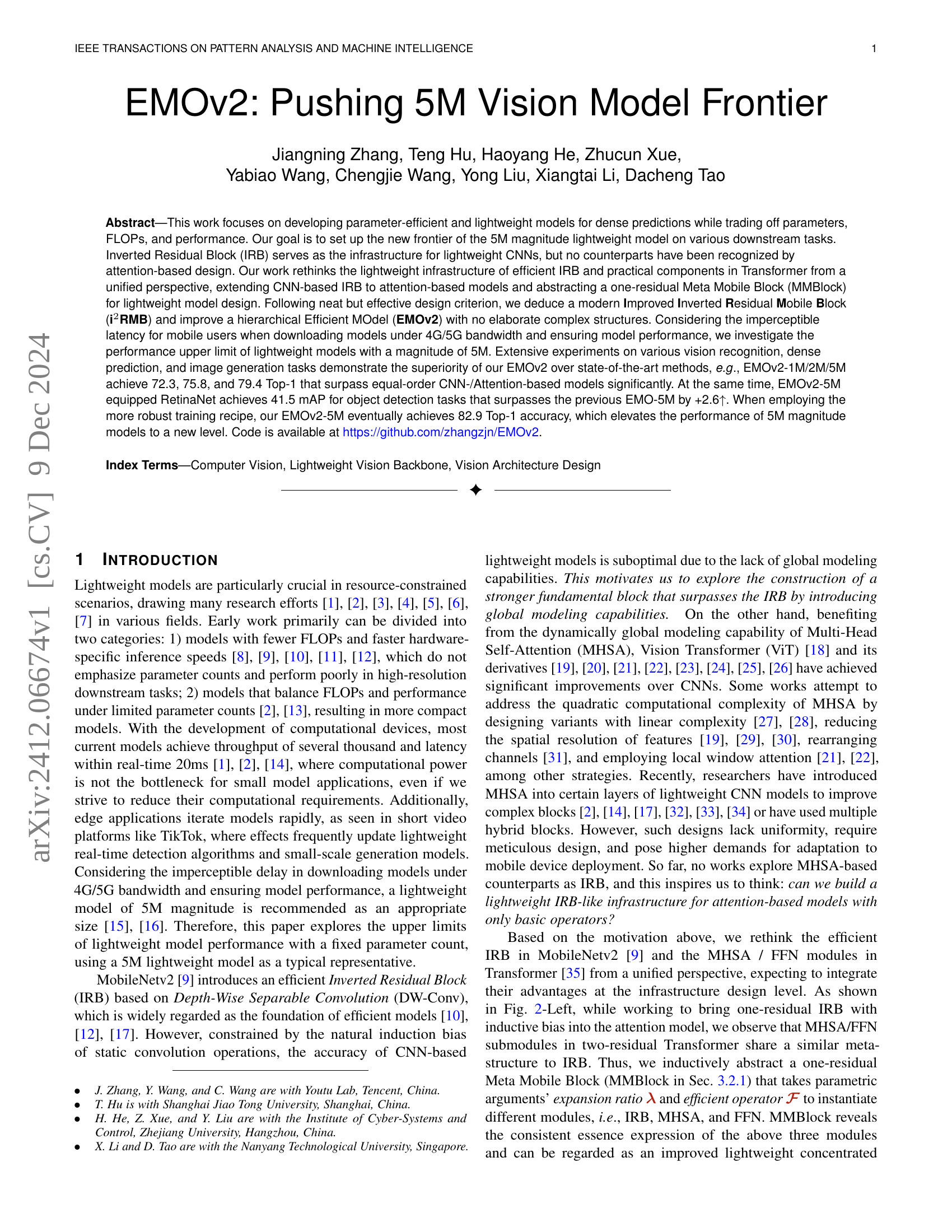
🔼 Figure 1 demonstrates EMOv2’s parameter efficiency and superior performance compared to other lightweight models. The top panel shows a plot of Top-1 accuracy versus the number of model parameters. It highlights that EMOv2 achieves higher accuracy with significantly fewer parameters than competing approaches, even when those approaches use more advanced training techniques (marked with an asterisk). The bottom panel illustrates the concept of effective receptive field (ERF). It compares the range of token interactions for various window attention mechanisms. EMOv2’s use of parameter-shared spanning attention results in a substantially larger ERF, signifying a greater ability to capture contextual information.
read the caption
Figure 1: Top: Performance vs. Parameters with concurrent methods. Our EMOv2 achieves significant accuracy with fewer parameters. Superscript ∗∗\ast∗: The comparison methods employ more robust training strategies described in their papers, while ours uses the strategy mentioned in Tab. XVII(e). Bottom: The range of token interactions varies with different window attention mechanisms. Our EMOv2, with parameter-shared spanning attention in Sec. 3.3.1, has a larger and correspondingly stronger Effective Receptive Field (ERF).
| Method vs. Criterion | ➀ | ➁ | ➂ | ➃ |
|---|---|---|---|---|
| MobileNet Series [8, 9, 32] | ✔ | ✔ | ✚ | ✘ |
| MobileViT Series [17, 14, 32] | ✚ | ✚ | ✚ | ✘ |
| EdgeNeXt [2] | ✚ | ✘ | ✔ | ✘ |
| EdgeViT [55] | ✔ | ✚ | ✚ | ✘ |
| RepViT [40] | ✔ | ✘ | ✔ | ✘ |
| EfficientFormerV2 [1] | ✔ | ✚ | ✔ | ✘ |
| EfficientVMamba [65] | ✘ | ✘ | ✚ | ✘ |
| MogaNet [50] | ✔ | ✔ | ✔ | ✘ |
| EMOv1 | ✔ | ✔ | ✔ | ✘ |
| EMOv2 | ✔ | ✔ | ✔ | ✔ |
🔼 This table compares several efficient models based on four criteria: Usability (ease of implementation and optimization), Uniformity (consistency and simplicity of model design), Efficiency and Effectiveness (balance between model parameters, computational cost, and accuracy), and Generalization (ability to adapt to various perception and generation tasks). Each criterion is marked as satisfied (✔), partially satisfied (✚), or unsatisfied (✘) for each model.
read the caption
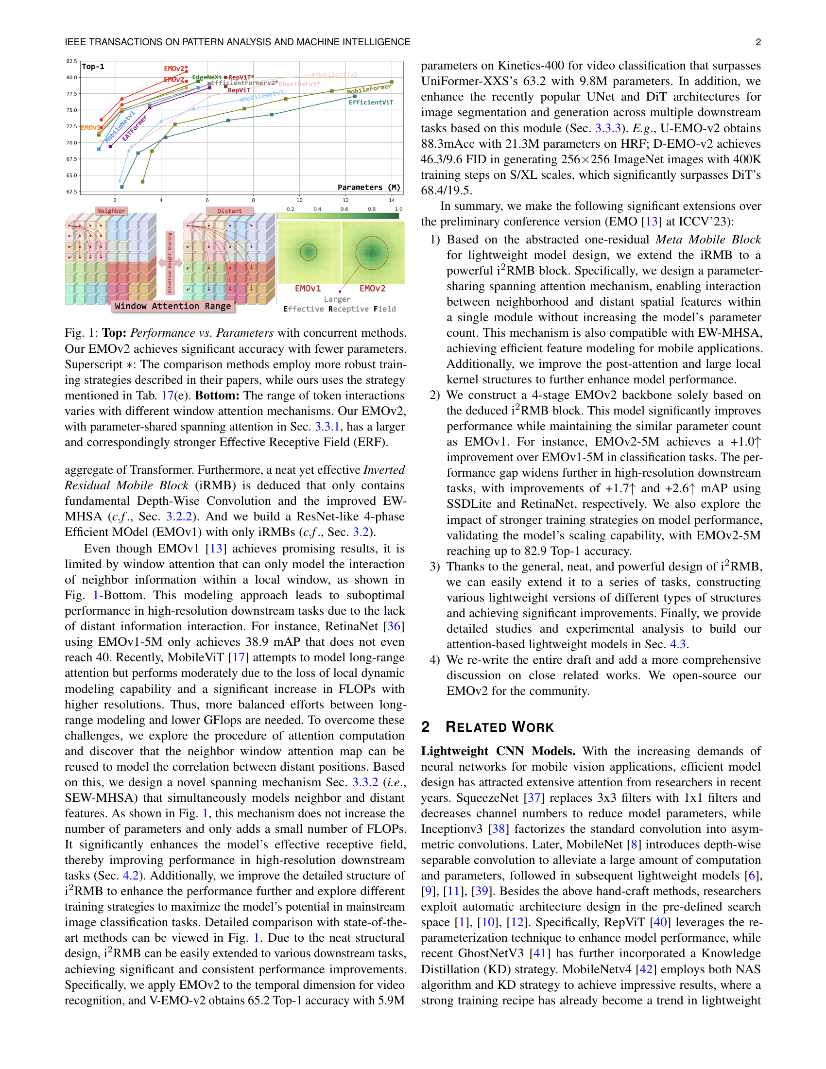
TABLE I: Criterion comparison for current efficient models. ➀: Usability; ➁: Uniformity; ➂: Efficiency and Effectiveness; ➃: Generalization. ✔: Satisfied. ✚: Partially satisfied. ✘: Unsatisfied.
In-depth insights#
Lightweight Design#
Lightweight model design in computer vision focuses on creating efficient architectures that minimize computational cost while maintaining high accuracy. Key strategies involve reducing model parameters (e.g., using depthwise separable convolutions, pruning), optimizing the number of floating-point operations (FLOPs) (e.g., through efficient attention mechanisms or architectural changes), and designing models suitable for deployment on resource-constrained devices. The trade-off between model size, computational cost, and accuracy is central to lightweight design. Challenges include balancing performance across various downstream tasks, addressing the inductive biases inherent in different network architectures (e.g., CNNs vs. Transformers), and developing training strategies suitable for limited resources. Successful approaches combine careful architectural design with efficient operator choices and innovative techniques (e.g., knowledge distillation, parameter sharing). Ultimately, lightweight design pushes the boundaries of what’s possible, enabling AI applications in areas previously restricted by computational limitations.
MMBlock Induction#
The MMBlock induction section is crucial as it lays the foundation for the paper’s core contribution: a unified, parameter-efficient building block for both CNNs and Transformers. The authors cleverly identify structural similarities between Inverted Residual Blocks (IRBs) and Transformer components (Multi-Head Self-Attention and Feed-Forward Networks). By abstracting these commonalities, they introduce the MMBlock, a meta-architecture that can be instantiated to create various specialized blocks by simply altering parameters. This unified perspective is innovative as it bridges the gap between CNNs and Transformers, which are traditionally treated as distinct architectural paradigms. The MMBlock’s significance stems from its potential for enhanced efficiency and generalizability. It allows for the creation of lightweight models by carefully selecting appropriate operators and expansion ratios within the MMBlock framework. This modularity simplifies the design process and fosters more streamlined, parameter-efficient networks. The success of this induction is ultimately validated by the subsequent development and performance evaluation of the EMOv2 architecture, which is entirely constructed using the MMBlock.
iRMB Enhancements#
The iRMB enhancements section would likely detail improvements made to the Inverted Residual Mobile Block (iRMB), a core building block of the proposed lightweight model. These improvements would likely focus on enhancing efficiency and accuracy. Potential enhancements include modifications to the depthwise convolution, the use of more sophisticated attention mechanisms (possibly replacing or augmenting the existing one), the introduction of new modules or connections to improve information flow, and optimizations of the block’s internal operations to reduce computational cost. The core goal would be to achieve a better balance between model size, computational complexity, and performance. A significant portion of this section might involve ablation studies, demonstrating the impact of individual modifications to the iRMB’s structure and quantifying their effect on accuracy and efficiency. Furthermore, the authors would probably discuss the design decisions behind the chosen enhancements, emphasizing their impact on the model’s overall efficiency and architectural elegance. The effectiveness of these improvements is expected to be evaluated through extensive experiments on various downstream tasks.
Empirical Analysis#
An empirical analysis section of a research paper would typically present the results of experiments designed to test the hypotheses or claims made in the paper. This would involve a detailed description of the experimental setup, including datasets used, methodologies employed, and any relevant parameters. The core of this section would focus on presenting the quantitative results obtained, often using tables and figures to display performance metrics, error rates, and statistical significance. A robust empirical analysis would not just report raw numbers but would also offer a thorough interpretation of the findings, comparing them to existing baselines or state-of-the-art methods. Crucially, it should discuss any limitations of the experimental design or findings, acknowledging potential biases or confounding factors. It might also include error analysis or sensitivity studies to better understand the robustness and generalizability of the results. Finally, a strong section would provide insightful conclusions based on the empirical evidence, clearly stating whether the initial hypotheses were supported and offering implications for future research. The goal is to provide a clear, convincing, and nuanced account of the empirical investigation.
Future Directions#
Future research could explore several promising avenues. Improving the efficiency of the attention mechanism is crucial; current methods, while efficient, still have limitations in terms of computational cost and memory usage, especially for high-resolution images and long sequences. Developing novel lightweight architectures that combine the strengths of CNNs and Transformers without their weaknesses remains a significant challenge. Exploring different training strategies is also essential. The success of EMOv2 highlights the potential impact of refined training methods on model performance and efficiency. Finally, expanding the application domain of the developed architecture to other computer vision tasks such as video understanding, 3D vision, and medical image analysis would be beneficial. Investigating the effect of different hardware platforms on model inference speed and energy efficiency is also important for real-world deployment. A particular focus should be given to model robustness and generalizability across various datasets and scenarios. Addressing these points will likely propel the field toward even more powerful and resource-efficient vision models.
More visual insights#
More on figures

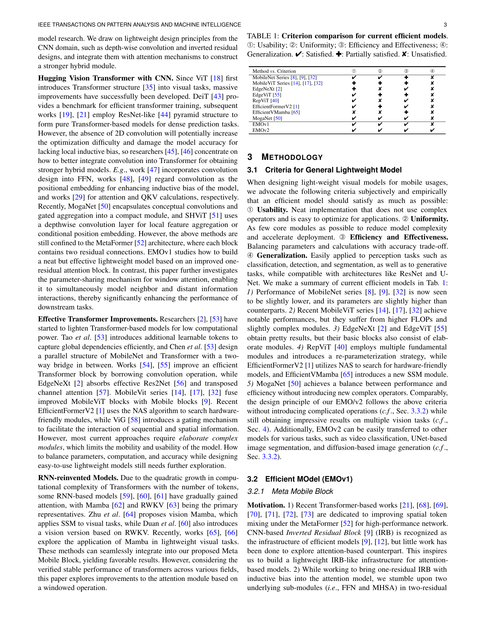
🔼 Figure 2 illustrates the core components and applications of the proposed EMOv2 model. The left panel shows the unified Meta-Mobile Block (MMBlock), a generalized building block derived from Multi-Head Self-Attention, Feed-Forward Networks, and Inverted Residual Blocks. This MMBlock can be instantiated into specific modules (like the Improved Inverted Residual Mobile Block or i2RMB) by adjusting parameters (expansion ratio λ and operator ℱ). The middle panel depicts how the 4-stage EMOv2 model is constructed using only the i2RMB, along with variations for different tasks such as video classification (V-EMO), encoder-decoder based image segmentation (U-EMO), and transformer replacement in DiT (D-EMO). The right panel provides a performance comparison of EMOv2 against other state-of-the-art models on various vision tasks.
read the caption
Figure 2: Left: Abstracted unified Meta-Mobile Block from Multi-Head Self-Attention, Feed-Forward Network [35], and Inverted Residual Block [9] (c.f. Sec 3.2.1). The inductive block can be deduced into specific modules using different expansion ratio λ𝜆\lambdaitalic_λ and efficient operator ℱℱ\mathcal{F}caligraphic_F. Middle: We construct a family of vision models based on our i2RMB module: 4-stage EMOv2, composed solely of the deduced i2RMB (c.f. Sec 3.2.2), for various perception tasks (image classification, detection, and segmentation in Sec. 4.2). Additionally, we introduce the temporally extended V-EMO for video classification, the U-EMO based on an encoder-decoder architecture, and D-EMO to replace the Transformer block in DiT [67]. These downstream models are typically built based on the i2RMB. Right: Performance comparison with different SoTAs on various tasks.

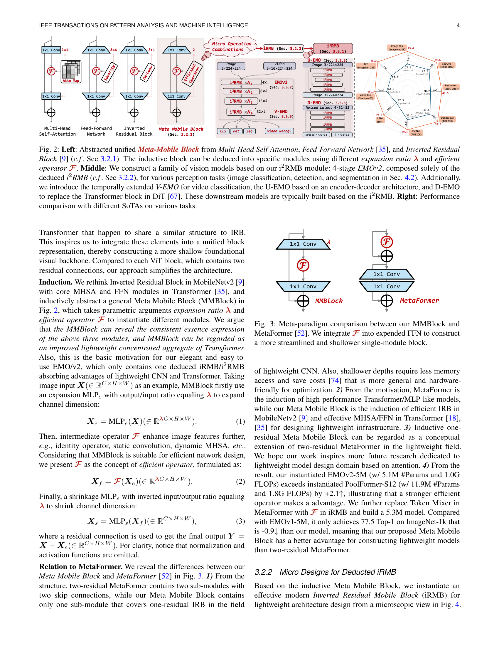
🔼 Figure 3 compares the proposed Meta Mobile Block (MMBlock) with the MetaFormer [52] architecture. The MMBlock simplifies the MetaFormer by integrating the efficient operator 𝓕 into the expanded feed-forward network (FFN), resulting in a single-module block that is both shallower and more streamlined than the two-module MetaFormer design. This streamlined design reduces computational complexity and improves efficiency.
read the caption
Figure 3: Meta-paradigm comparison between our MMBlock and MetaFormer [52]. We integrate 𝓕𝓕{\color[rgb]{0.69140625,0.140625,0.09375}\definecolor[named]{pgfstrokecolor}{% rgb}{0.69140625,0.140625,0.09375}\bm{\mathcal{F}}}bold_caligraphic_F into expended FFN to construct a more streamlined and shallower single-module block.

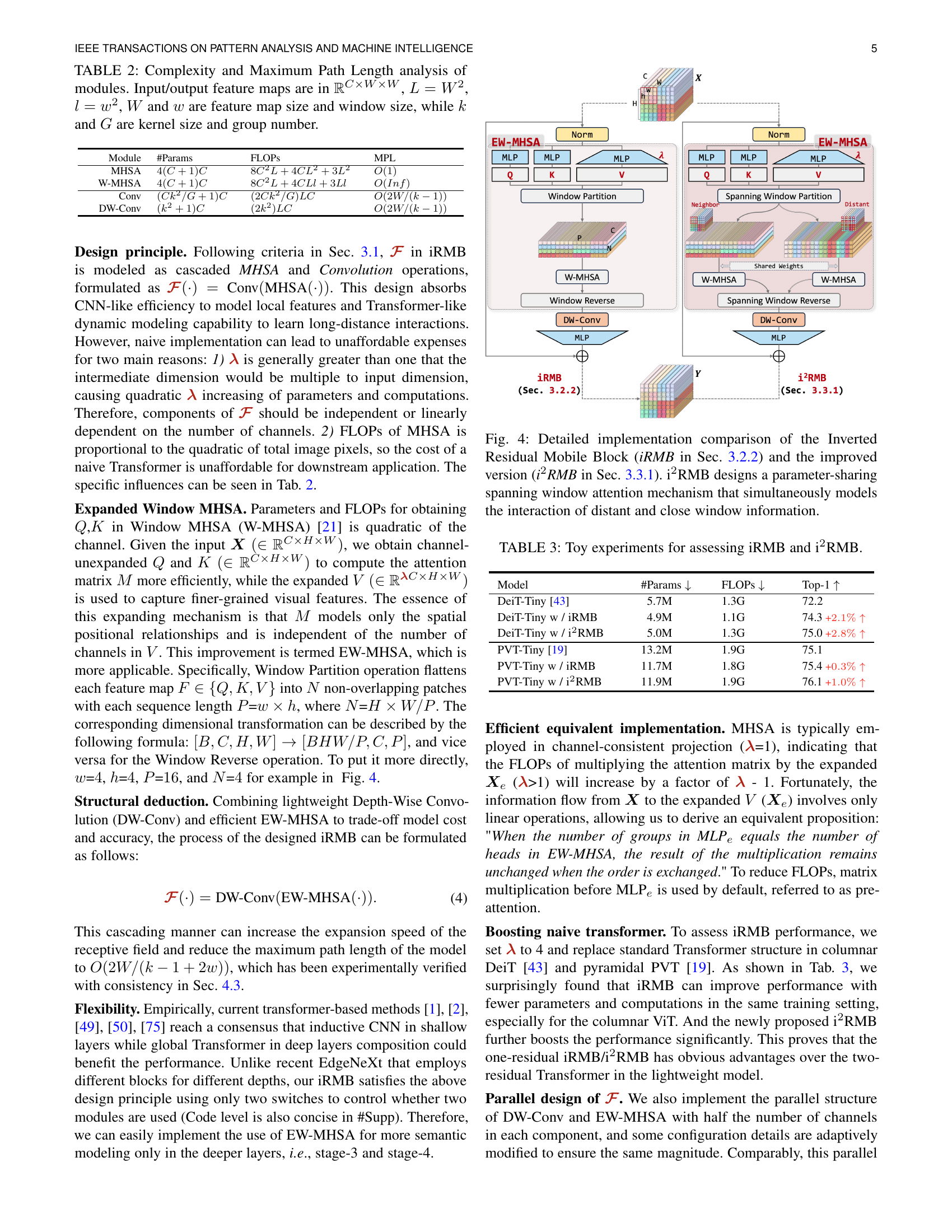
🔼 Figure 4 illustrates the architectural differences between the original Inverted Residual Mobile Block (iRMB) and its enhanced counterpart, the i2RMB. The iRMB uses a standard windowed attention mechanism, processing only information within a limited spatial window. The improved i2RMB introduces a parameter-sharing spanning window attention mechanism. This enhancement allows the i2RMB to simultaneously consider both local (nearby) and distant spatial relationships within the input feature map, leading to a more comprehensive and potentially more accurate understanding of the context. This is achieved without a significant increase in model parameters.
read the caption
Figure 4: Detailed implementation comparison of the Inverted Residual Mobile Block (iRMB in Sec. 3.2.2) and the improved version (i2RMB in Sec. 3.3.1). i2RMB designs a parameter-sharing spanning window attention mechanism that simultaneously models the interaction of distant and close window information.

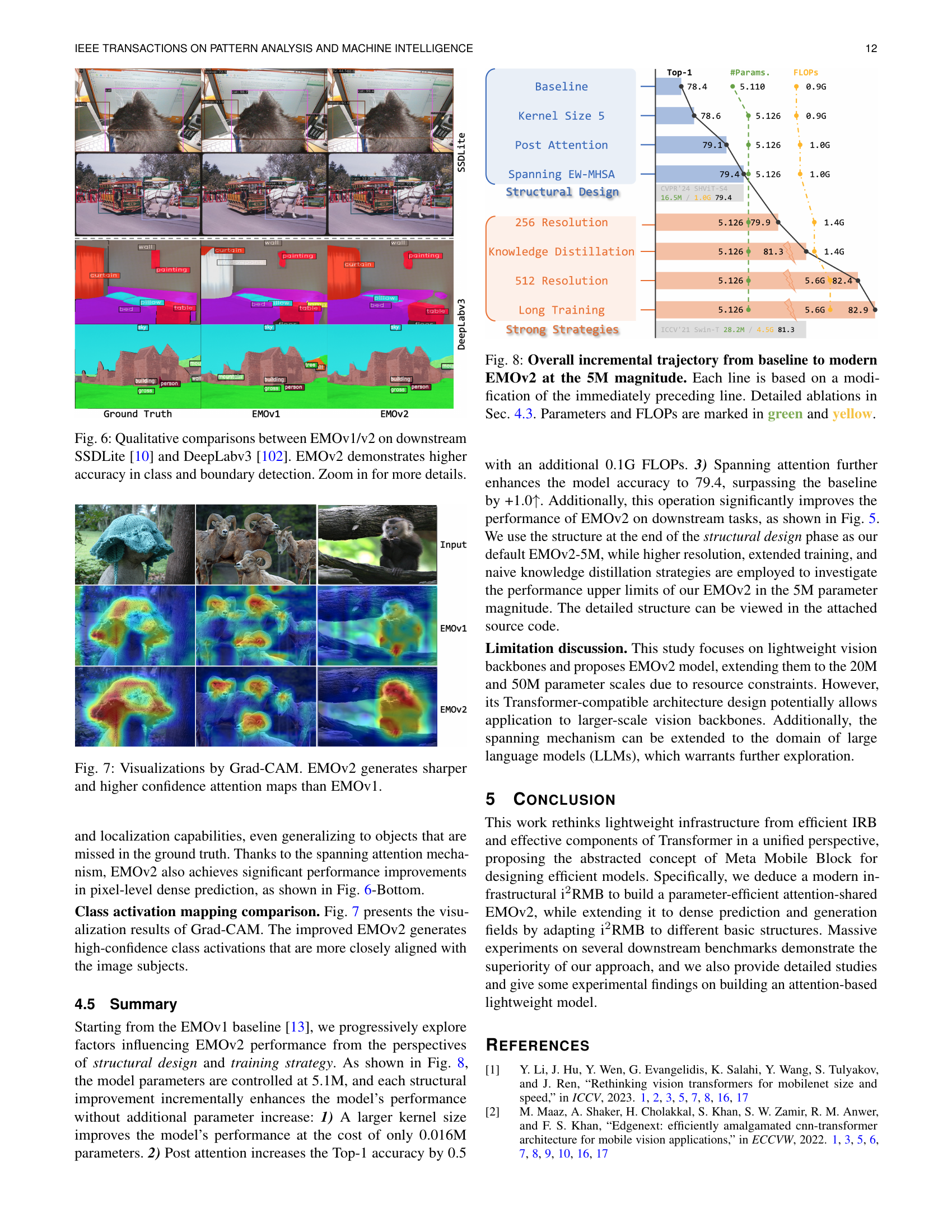
🔼 This figure compares the performance of EMOv2-5M and EMOv1-5M on various downstream tasks, including object detection using SSDLite and RetinaNet, and semantic segmentation using DeepLabv3, Semantic FPN, and PSPNet. It visually demonstrates the improvement in accuracy achieved by EMOv2-5M over EMOv1-5M in these tasks. The improvements are shown as bar chart showing the mAP for object detection and mIoU for semantic segmentation.
read the caption
Figure 5: Downstream gains of EMOv2-5M over EMOv1-5M.

🔼 This figure shows a comparison of the Inverted Residual Mobile Block (iRMB) and its improved version (i2RMB). The iRMB uses a cascaded design of Multi-Head Self-Attention (MHSA) and convolution operations. The i2RMB introduces a parameter-sharing spanning window attention mechanism which models both local and distant features. The figure details the architectural differences and highlights the efficiency and effectiveness of the i2RMB.
read the caption
(a)

🔼 This figure displays a comparison of different attention mechanisms’ implementations within the Inverted Residual Mobile Block (iRMB). It shows the original Window MHSA, a modified version called Spanning Window MHSA (SEW-MHSA), and their respective reverse operations. SEW-MHSA is highlighted as the improved method that simultaneously models both near and distant feature interactions, aiming to overcome limitations of only modeling local neighbor interactions within a smaller window. The diagram visually depicts the data flow and window partitioning strategies for each approach.
read the caption
(b)

🔼 This figure shows a comparison of the improved Inverted Residual Mobile Block (i2RMB) and the original iRMB. The i2RMB introduces a parameter-sharing spanning window attention mechanism. This mechanism efficiently models both local (neighbor) and long-range (distant) feature interactions simultaneously, unlike the original iRMB which focuses solely on local interactions within a window. This improvement is crucial for enhancing the model’s effective receptive field, especially in high-resolution tasks. The diagram visually details the architectural differences between the two blocks, illustrating the added component that makes the i2RMB more efficient and powerful.
read the caption
(c)
More on tables
| Module | #Params | FLOPs | MPL |
|---|---|---|---|
| MHSA | 4(C+1)C | 8C2L+4CL2+3L2 | O(1) |
| W-MHSA | 4(C+1)C | 8C2L+4CLl+3Ll | O(Inf) |
| Conv | (Ck2/G+1)C | (2Ck2/G)LC | O(2W/(k-1)) |
| DW-Conv | (k2+1)C | (2k2)LC | O(2W/(k-1)) |
🔼 This table details the computational complexity and maximum path length of different modules used in the paper, specifically focusing on the relationship between parameters, FLOPs (floating-point operations), and the dimensions of the input feature maps. The variables defined (C, W, w, k, G, L, l) represent the number of channels, feature map width/height, window width/height, kernel size, number of groups in convolution, total number of pixels in feature map, and total number of pixels in window, respectively. Understanding these relationships is crucial for evaluating the efficiency of different components in lightweight model design.
read the caption
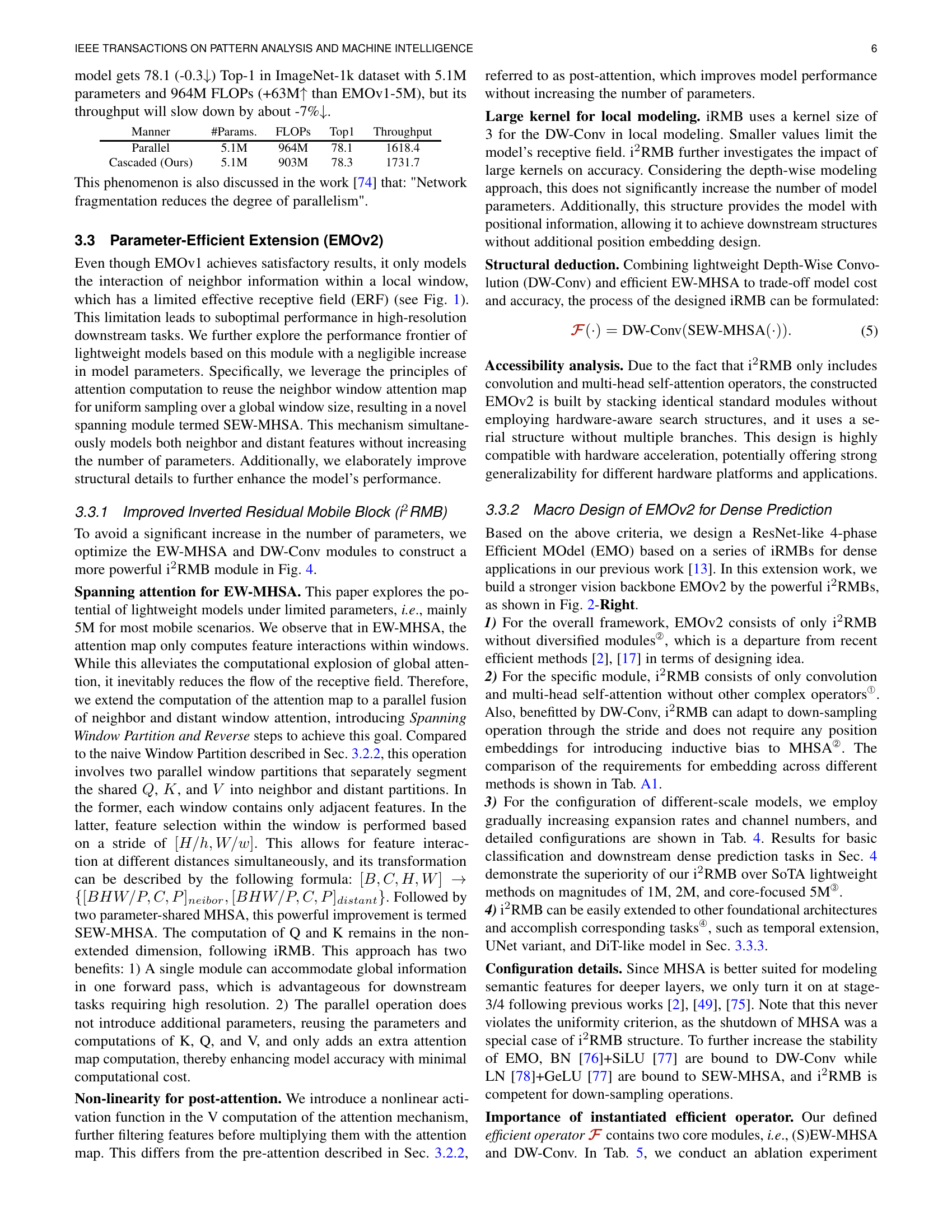
TABLE II: Complexity and Maximum Path Length analysis of modules. Input/output feature maps are in ℝC×W×Wsuperscriptℝ𝐶𝑊𝑊\mathbb{R}^{C\times W\times W}blackboard_R start_POSTSUPERSCRIPT italic_C × italic_W × italic_W end_POSTSUPERSCRIPT, L=W2𝐿superscript𝑊2L=W^{2}italic_L = italic_W start_POSTSUPERSCRIPT 2 end_POSTSUPERSCRIPT, l=w2𝑙superscript𝑤2l=w^{2}italic_l = italic_w start_POSTSUPERSCRIPT 2 end_POSTSUPERSCRIPT, W𝑊Witalic_W and w𝑤witalic_w are feature map size and window size, while k𝑘kitalic_k and G𝐺Gitalic_G are kernel size and group number.
| Model | #Params ↓ | FLOPs ↓ | Top-1 ↑ |
|---|---|---|---|
| DeiT-Tiny [43] | 5.7M | 1.3G | 72.2 |
| DeiT-Tiny w / iRMB | 4.9M | 1.1G | 74.3 +2.1%↑ |
| DeiT-Tiny w / i²RMB | 5.0M | 1.3G | 75.0 +2.8%↑ |
| PVT-Tiny [19] | 13.2M | 1.9G | 75.1 |
| PVT-Tiny w / iRMB | 11.7M | 1.8G | 75.4 +0.3%↑ |
| PVT-Tiny w / i²RMB | 11.9M | 1.9G | 76.1 +1.0%↑ |
🔼 This table presents the results of toy experiments conducted to evaluate the performance of two types of Inverted Residual Mobile Blocks (iRMB and i2RMB). The experiments involve replacing the transformer blocks in DeiT-Tiny and PVT-Tiny models with the iRMB and i2RMB blocks respectively. The table shows the number of parameters, FLOPs, and Top-1 accuracy achieved by each model configuration.
read the caption
TABLE III: Toy experiments for assessing iRMB and i2RMB.
| Manner | #Params. | FLOPs | Top1 | Throughput |
|---|---|---|---|---|
| Parallel | 5.1M | 964M | 78.1 | 1618.4 |
| Cascaded (Ours) | 5.1M | 903M | 78.3 | 1731.7 |
🔼 This table details the core configurations used to create different versions of the EMOv2 model. These configurations control aspects of the model’s architecture, allowing for variations in the number of parameters and computational cost, thereby influencing the model’s performance and suitability for different resource constraints. The configurations specify the depth, embedding dimension, and expansion ratio of the model’s components.
read the caption
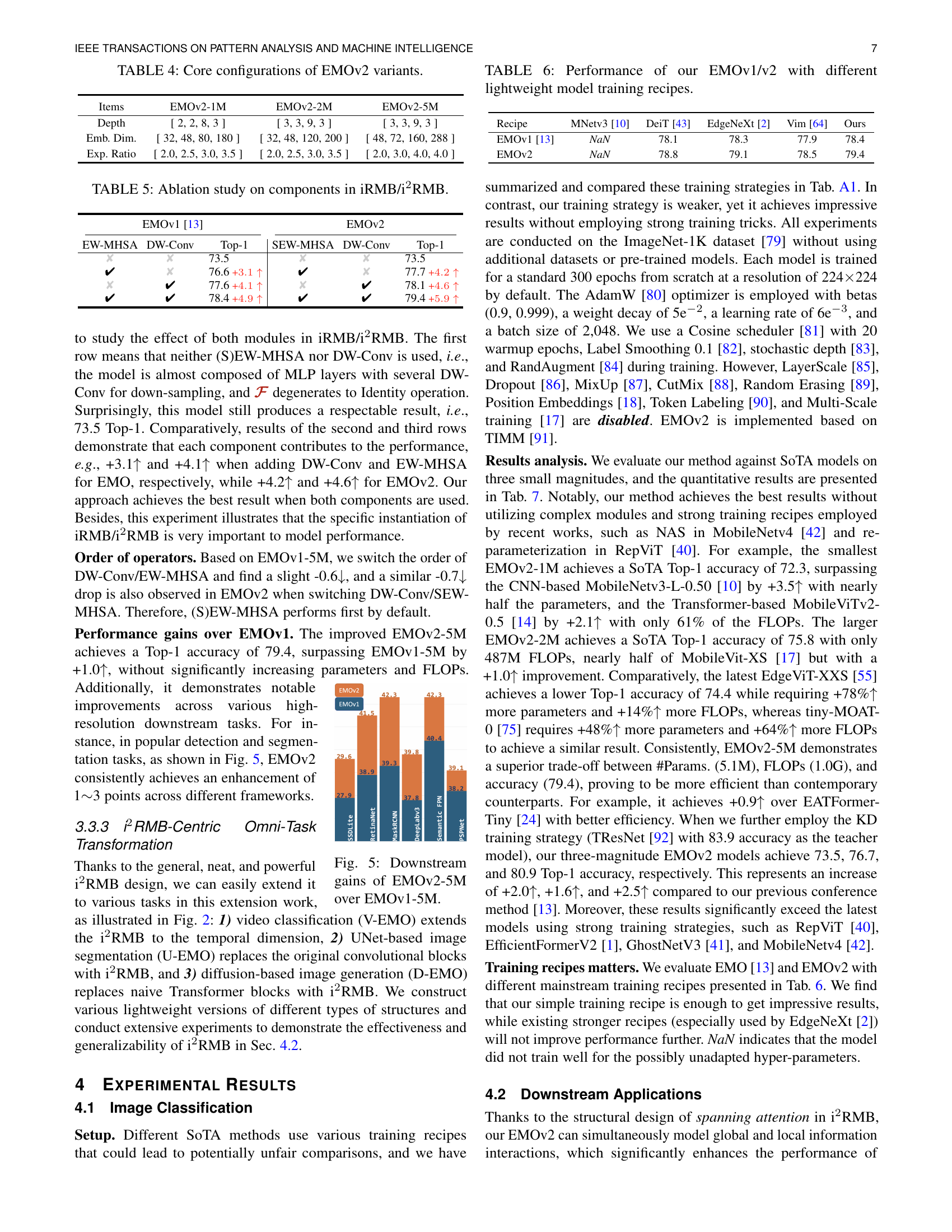
TABLE IV: Core configurations of EMOv2 variants.
| Items | EMoV2-1M | EMoV2-2M | EMoV2-5M |
|---|---|---|---|
| Depth | [ 2, 2, 8, 3 ] | [ 3, 3, 9, 3 ] | [ 3, 3, 9, 3 ] |
| Emb. Dim. | [ 32, 48, 80, 180 ] | [ 32, 48, 120, 200 ] | [ 48, 72, 160, 288 ] |
| Exp. Ratio | [ 2.0, 2.5, 3.0, 3.5 ] | [ 2.0, 2.5, 3.0, 3.5 ] | [ 2.0, 3.0, 4.0, 4.0 ] |
🔼 This table presents an ablation study analyzing the impact of individual components within the Improved Inverted Residual Mobile Block (iRMB) and its enhanced version, the i2RMB. It shows the performance (Top-1 accuracy) achieved by removing either the EW-MHSA (Expanded Window Multi-Head Self-Attention) or the DW-Conv (Depthwise Convolution) component, or both, from the baseline model. This allows for a quantitative assessment of the contribution of each component to the overall model accuracy. The experiment is conducted for both EMOv1 and EMOv2.
read the caption
TABLE V: Ablation study on components in iRMB/i2RMB.
| EMOV1 [13] | EMOV2 | |||||
|---|---|---|---|---|---|---|
| EW-MHSA | DW-Conv | 73.5 | SEW-MHSA | DW-Conv | 73.5 | |
| ✘ | ✘ | 73.5 | ✘ | ✘ | 73.5 | |
| ✔ | ✘ | 76.6+3.1↑ | ✔ | ✘ | 77.7+4.2↑ | |
| ✘ | ✔ | 77.6+4.1↑ | ✘ | ✔ | 78.1+4.6↑ | |
| ✔ | ✔ | 78.4+4.9↑ | ✔ | ✔ | 79.4+5.9↑ |
🔼 This table compares the performance of EMOv1 and EMOv2 models trained using various lightweight training recipes. It highlights how different training methodologies impact the final accuracy of the models, demonstrating their robustness or sensitivity to different training strategies. The results are likely presented as top-1 accuracy on a benchmark dataset like ImageNet.
read the caption
TABLE VI: Performance of our EMOv1/v2 with different lightweight model training recipes.
| Recipe | MNetv3 [10] | DeiT [43] | EdgeNeXt [2] | Vim [64] | Ours |
|---|---|---|---|---|---|
| EMOV1 [13] | NaN | 78.1 | 78.3 | 77.9 | 78.4 |
| EMOV2 | NaN | 78.8 | 79.1 | 78.5 | 79.4 |
🔼 Table VII presents a comparison of classification performance on the ImageNet-1K dataset for various lightweight models, specifically focusing on those with parameter counts around 1M, 2M, and 5M. The table categorizes models based on their architecture: CNN-based (white background), Transformer-based (gray background), RNN-based (orange background), and the authors’ proposed EMO models (blue background). Results from the original papers are shown in gray, while the authors highlight their recommended models in bold. Key details, such as the number of parameters (#Params) and floating-point operations (FLOPS), are included, along with Top-1 accuracy. Additional notes clarify the use of specialized training techniques like Neural Architecture Search (NAS), knowledge distillation (KD), and re-parameterization, allowing for better interpretation of the results.
read the caption
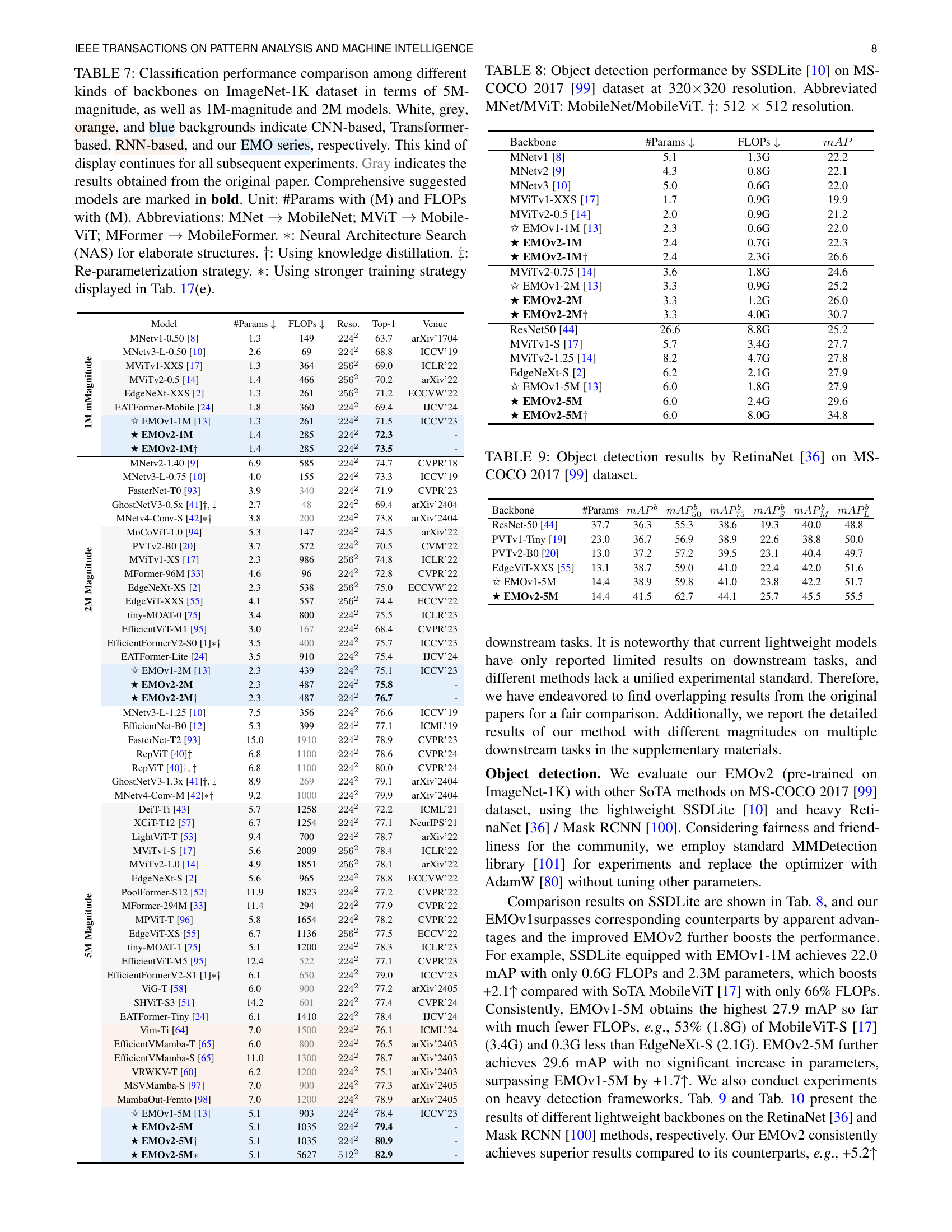
TABLE VII: Classification performance comparison among different kinds of backbones on ImageNet-1K dataset in terms of 5M-magnitude, as well as 1M-magnitude and 2M models. White, grey, orange, and blue backgrounds indicate CNN-based, Transformer-based, RNN-based, and our EMO series, respectively. This kind of display continues for all subsequent experiments. Gray indicates the results obtained from the original paper. Comprehensive suggested models are marked in bold. Unit: #Params with (M) and FLOPs with (M). Abbreviations: MNet →→\rightarrow→ MobileNet; MViT →→\rightarrow→ MobileViT; MFormer →→\rightarrow→ MobileFormer. ∗∗\ast∗: Neural Architecture Search (NAS) for elaborate structures. ††\dagger†: Using knowledge distillation. ‡‡\ddagger‡: Re-parameterization strategy. ∗∗\ast∗: Using stronger training strategy displayed in Tab. XVII(e).
| Model | #Params ↓ | FLOPs ↓ | Reso. | Top-1 | Venue | |
|---|---|---|---|---|---|---|
 | MNetv1-0.50 [8] | 1.3 | 149 | 2242 | 63.7 | arXiv’1704 |
| MNetv3-L-0.50 [10] | 2.6 | 69 | 2242 | 68.8 | ICCV’19 | |
| MViTv1-XXS [17] | 1.3 | 364 | 2562 | 69.0 | ICLR’22 | |
| MViTv2-0.5 [14] | 1.4 | 466 | 2562 | 70.2 | arXiv’22 | |
| EdgeNeXt-XXS [2] | 1.3 | 261 | 2562 | 71.2 | ECCVW’22 | |
| EATFormer-Mobile [24] | 1.8 | 360 | 2242 | 69.4 | IJCV’24 | |
| ✩ EMOV1-1M [13] | 1.3 | 261 | 2242 | 71.5 | ICCV’23 | |
| ★ EMOv2-1M | 1.4 | 285 | 2242 | 72.3 | - | |
| ★ EMOv2-1M† | 1.4 | 285 | 2242 | 73.5 | - | |
 | MNetv2-1.40 [9] | 6.9 | 585 | 2242 | 74.7 | CVPR’18 |
| MNetv3-L-0.75 [10] | 4.0 | 155 | 2242 | 73.3 | ICCV’19 | |
| FasterNet-T0 [93] | 3.9 | 340 | 2242 | 71.9 | CVPR’23 | |
| GhostNetV3-0.5x [41] †,‡ | 2.7 | 48 | 2242 | 69.4 | arXiv’2404 | |
| MNetv4-Conv-S [42] ∗† | 3.8 | 200 | 2242 | 73.8 | arXiv’2404 | |
| MoCoViT-1.0 [94] | 5.3 | 147 | 2242 | 74.5 | arXiv’22 | |
| PVTv2-B0 [20] | 3.7 | 572 | 2242 | 70.5 | CVM’22 | |
| MViTv1-XS [17] | 2.3 | 986 | 2562 | 74.8 | ICLR’22 | |
| MFormer-96M [33] | 4.6 | 96 | 2242 | 72.8 | CVPR’22 | |
| EdgeNeXt-XS [2] | 2.3 | 538 | 2562 | 75.0 | ECCVW’22 | |
| EdgeViT-XXS [55] | 4.1 | 557 | 2562 | 74.4 | ECCV’22 | |
| tiny-MOAT-0 [75] | 3.4 | 800 | 2242 | 75.5 | ICLR’23 | |
| EfficientViT-M1 [95] | 3.0 | 167 | 2242 | 68.4 | CVPR’23 | |
| EfficientFormerV2-S0 [1] ∗† | 3.5 | 400 | 2242 | 75.7 | ICCV’23 | |
| EATFormer-Lite [24] | 3.5 | 910 | 2242 | 75.4 | IJCV’24 | |
| ✩ EMOV1-2M [13] | 2.3 | 439 | 2242 | 75.1 | ICCV’23 | |
| ★ EMOv2-2M | 2.3 | 487 | 2242 | 75.8 | - | |
| ★ EMOv2-2M† | 2.3 | 487 | 2242 | 76.7 | - | |
| MNetv3-L-1.25 [10] | 7.5 | 356 | 2242 | 76.6 | ICCV’19 | |
| EfficientNet-B0 [12] | 5.3 | 399 | 2242 | 77.1 | ICML’19 | |
| FasterNet-T2 [93] | 15.0 | 1910 | 2242 | 78.9 | CVPR’23 | |
| RepViT [40] ‡ | 6.8 | 1100 | 2242 | 78.6 | CVPR’24 | |
| RepViT [40] †,‡ | 6.8 | 1100 | 2242 | 80.0 | CVPR’24 | |
| GhostNetV3-1.3x [41] †,‡ | 8.9 | 269 | 2242 | 79.1 | arXiv’2404 | |
| MNetv4-Conv-M [42] ∗† | 9.2 | 1000 | 2242 | 79.9 | arXiv’2404 | |
| DeiT-Ti [43] | 5.7 | 1258 | 2242 | 72.2 | ICML’21 | |
| XCiT-T12 [57] | 6.7 | 1254 | 2242 | 77.1 | NeurIPS’21 | |
| LightViT-T [53] | 9.4 | 700 | 2242 | 78.7 | arXiv’22 | |
| MViTv1-S [17] | 5.6 | 2009 | 2562 | 78.4 | ICLR’22 | |
| MViTv2-1.0 [14] | 4.9 | 1851 | 2562 | 78.1 | arXiv’22 | |
| EdgeNeXt-S [2] | 5.6 | 965 | 2242 | 78.8 | ECCVW’22 | |
| PoolFormer-S12 [52] | 11.9 | 1823 | 2242 | 77.2 | CVPR’22 | |
| MFormer-294M [33] | 11.4 | 294 | 2242 | 77.9 | CVPR’22 | |
| MPViT-T [96] | 5.8 | 1654 | 2242 | 78.2 | CVPR’22 | |
| EdgeViT-XS [55] | 6.7 | 1136 | 2562 | 77.5 | ECCV’22 | |
| tiny-MOAT-1 [75] | 5.1 | 1200 | 2242 | 78.3 | ICLR’23 | |
| EfficientViT-M5 [95] | 12.4 | 522 | 2242 | 77.1 | CVPR’23 | |
| ✩ EMOV1-5M [13] | 5.1 | 903 | 2242 | 78.4 | ICCV’23 | |
| ★ EMOv2-5M | 5.1 | 1035 | 2242 | 79.4 | - | |
| ★ EMOv2-5M∗ | 5.1 | 5627 | 5122 | 82.9 | - | |
| Vim-Ti [64] | 7.0 | 1500 | 2242 | 76.1 | ICML’24 | |
| EfficientVMamba-T [65] | 6.0 | 800 | 2242 | 76.5 | arXiv’2403 | |
| EfficientVMamba-S [65] | 11.0 | 1300 | 2242 | 78.7 | arXiv’2403 | |
| VRWKV-T [60] | 6.2 | 1200 | 2242 | 75.1 | arXiv’2403 | |
| MSVMamba-S [97] | 7.0 | 900 | 2242 | 77.3 | arXiv’2405 | |
| MambaOut-Femto [98] | 7.0 | 1200 | 2242 | 78.9 | arXiv’2405 |
🔼 This table presents the performance of different models on the object detection task using the SSDLite [10] framework. The models are evaluated on the MS-COCO 2017 [99] dataset at a resolution of 320x320 pixels. The results are shown in terms of mean Average Precision (mAP). For easier reference, MobileNet and MobileViT models are abbreviated as MNet and MViT, respectively. Some models were additionally evaluated at a higher resolution of 512x512 pixels; these results are marked with a † symbol.
read the caption
TABLE VIII: Object detection performance by SSDLite [10] on MS-COCO 2017 [99] dataset at 320×\times×320 resolution. Abbreviated MNet/MViT: MobileNet/MobileViT. ††\dagger†: 512 ×\times× 512 resolution.
| Backbone | #Params ↓ | FLOPs ↓ | mAP |
|---|---|---|---|
| MNetv1 [8] | 5.1 | 1.3G | 22.2 |
| MNetv2 [9] | 4.3 | 0.8G | 22.1 |
| MNetv3 [10] | 5.0 | 0.6G | 22.0 |
| MViTv1-XXS [17] | 1.7 | 0.9G | 19.9 |
| MViTv2-0.5 [14] | 2.0 | 0.9G | 21.2 |
| ✩ EMOV1-1M [13] | 2.3 | 0.6G | 22.0 |
| ★ EMOv2-1M | 2.4 | 0.7G | 22.3 |
| ★ EMOv2-1M† | 2.4 | 2.3G | 26.6 |
| MViTv2-0.75 [14] | 3.6 | 1.8G | 24.6 |
| ✩ EMOV1-2M [13] | 3.3 | 0.9G | 25.2 |
| ★ EMOv2-2M | 3.3 | 1.2G | 26.0 |
| ★ EMOv2-2M† | 3.3 | 4.0G | 30.7 |
| ResNet50 [44] | 26.6 | 8.8G | 25.2 |
| MViTv1-S [17] | 5.7 | 3.4G | 27.7 |
| MViTv2-1.25 [14] | 8.2 | 4.7G | 27.8 |
| EdgeNeXt-S [2] | 6.2 | 2.1G | 27.9 |
| ✩ EMOV1-5M [13] | 6.0 | 1.8G | 27.9 |
| ★ EMOv2-5M | 6.0 | 2.4G | 29.6 |
| ★ EMOv2-5M† | 6.0 | 8.0G | 34.8 |
🔼 Table IX presents the performance comparison of different lightweight backbones on the MS COCO 2017 object detection dataset using the RetinaNet framework. The table shows the mean Average Precision (mAP) results for various object sizes (small, medium, large) and overall mAP, along with the number of parameters and FLOPs (floating point operations) for each backbone model. This allows for a quantitative comparison of the trade-off between model efficiency and detection accuracy across different lightweight architectures.
read the caption
TABLE IX: Object detection results by RetinaNet [36] on MS-COCO 2017 [99] dataset.
| Backbone | #Params | mAPb | mAPb50 | mAPb75 | mAPbS | mAPbM | mAPbL |
|---|---|---|---|---|---|---|---|
| ResNet-50 [44] | 37.7 | 36.3 | 55.3 | 38.6 | 19.3 | 40.0 | 48.8 |
| PVTv1-Tiny [19] | 23.0 | 36.7 | 56.9 | 38.9 | 22.6 | 38.8 | 50.0 |
| PVTv2-B0 [20] | 13.0 | 37.2 | 57.2 | 39.5 | 23.1 | 40.4 | 49.7 |
| EdgeViT-XXS [55] | 13.1 | 38.7 | 59.0 | 41.0 | 22.4 | 42.0 | 51.6 |
| ✩ EMOV1-5M | 14.4 | 38.9 | 59.8 | 41.0 | 23.8 | 42.2 | 51.7 |
| ★ EMOV2-5M | 14.4 | 41.5 | 62.7 | 44.1 | 25.7 | 45.5 | 55.5 |
🔼 Table A3 presents a comprehensive comparison of object detection performance achieved by the Mask R-CNN model [100] using different backbones on the MS-COCO 2017 dataset [99]. It details the performance metrics, specifically mean Average Precision (mAP) across various Intersection over Union (IoU) thresholds, for different model sizes (1M, 2M, 5M, and 20M parameters) of the EMOv2 architecture. The table allows for a detailed analysis of how the EMOv2 backbone impacts object detection accuracy at different scales and under different model configurations (with and without the enhanced training strategy denoted by ‘+’).
read the caption
TABLE X: Object detection results by Mask RCNN [100] on MS-COCO 2017 [99] dataset.
| Backbone | #Params ↓ | mAPb | mAPb50 | mAPb75 | mAPbS | mAPbM | mAPbL | mAPm | mAPm50 | mAPm75 | mAPmS | mAPmM | mAPmL | |
|---|---|---|---|---|---|---|---|---|---|---|---|---|---|---|
| PVT-Tiny [19] | 33.0 | 36.7 | 59.2 | 39.3 | - | - | - | 35.1 | 56.7 | 37.3 | - | - | - | |
| PVTv2-B0 [20] | 23.0 | 38.2 | 60.5 | 40.7 | - | - | - | 36.2 | 57.8 | 38.6 | - | - | - | |
| PoolFormer-S12 [52] | 31.0 | 37.3 | 59.0 | 40.1 | - | - | - | 34.6 | 55.8 | 36.9 | - | - | - | |
| MPViT-T [96] | 28.0 | 42.2 | 64.2 | 45.8 | - | - | - | 39.0 | 61.4 | 41.8 | - | - | - | |
| EATFormer-Tiny [24] | 25.9 | 42.3 | 64.7 | 46.2 | 25.5 | 45.5 | 55.1 | 39.0 | 61.5 | 42.0 | 22.4 | 42.0 | 52.7 | |
| ✩ EMOV1-5M | 24.8 | 39.3 | 61.7 | 42.4 | 23.5 | 42.3 | 51.1 | 36.4 | 58.4 | 38.7 | 18.2 | 39.0 | 52.6 | |
| ★ EMOV2-5M | 24.8 | 42.3 | 64.3 | 46.3 | 25.8 | 45.6 | 56.3 | 39.0 | 61.4 | 42.1 | 20.0 | 41.8 | 57.0 |
🔼 Table XI presents a comparison of semantic segmentation performance achieved by four different models (DeepLabv3, Semantic FPN, SegFormer, and PSPNet) on the ADE20K dataset. The comparison is made using the same resolution (512x512) for all models, allowing for a direct assessment of their performance under the same conditions. The table likely shows metrics such as mean Intersection over Union (mIoU), accuracy, and other relevant performance measures for each model, providing a quantitative comparison of the relative strengths of the various approaches to semantic segmentation.
read the caption
TABLE XI: Semantic segmentation results by DeepLabv3 [102], Semantic FPN [103], SegFormer [104], and PSPNet [105] on ADE20K [106] dataset at 512×\times×512 resolution.
| Backbone | #Params ↓ | FLOPs ↓ | mIoU |
|---|---|---|---|
| DeepLabv3 [102] | |||
| MViTv2-0.5 | 6.3 | 26.1G | 31.9 |
| MViTv3-0.5 | 6.3 | - | 33.5 |
| ✩ EMOv1-1M | 5.6 | 2.4G | 33.5 |
| ★ EMOv2-1M | 5.6 | 3.3G | 34.6 |
| MNetv2 | 18.7 | 75.4G | 34.1 |
| MViTv2-0.75 | 9.6 | 40.0G | 34.7 |
| MViTv3-0.75 | 9.7 | - | 36.4 |
| ✩ EMOv1-2M | 6.9 | 3.5G | 35.3 |
| ★ EMOv2-2M | 6.6 | 5.0G | 36.8 |
| MViTv2-1.0 | 13.4 | 56.4G | 37.0 |
| MViTv3-1.0 | 13.6 | - | 39.1 |
| ✩ EMOv1-5M | 10.3 | 5.8G | 37.8 |
| ★ EMOv2-5M | 9.9 | 9.1G | 39.8 |
| Semantic FPN [103] | |||
| ResNet-18 | 15.5 | 32.2G | 32.9 |
| ✩ EMOv1-1M | 5.2 | 22.5G | 34.2 |
| ★ EMOv2-1M | 5.3 | 23.4G | 37.1 |
| ResNet-50 | 28.5 | 45.6G | 36.7 |
| PVTv1-Tiny | 17.0 | 33.2G | 35.7 |
| PVTv2-B0 | 7.6 | 25.0G | 37.2 |
| ✩ EMOv1-2M | 6.2 | 23.5G | 37.3 |
| ★ EMOv2-2M | 6.2 | 25.1G | 39.9 |
| ResNet-101 | 47.5 | 65.1G | 38.8 |
| ResNeXt-101 | 47.1 | 64.7G | 39.7 |
| PVTv1-Small | 28.2 | 44.5G | 39.8 |
| EdgeViT-XXS | 7.9 | 24.4G | 39.7 |
| EdgeViT-XS | 10.6 | 27.7G | 41.4 |
| PVTv2-B1 | 17.8 | 34.2G | 42.5 |
| ✩ EMOv1-5M | 8.9 | 25.8G | 40.4 |
| ★ EMOv2-5M | 8.9 | 29.1G | 42.3 |
| SegFormer [104] | |||
| MiT-B0 | 3.8 | 8.4G | 37.4 |
| ★ EMOv2-2M | 2.6 | 10.3G | 40.2 |
| MiT-B1 | 13.7 | 15.9G | 42.2 |
| ★ EMOv2-5M | 5.3 | 14.4G | 43.0 |
| PSPNet [105] | |||
| MNetv2 | 13.7 | 53.1G | 29.7 |
| MViTv2-0.5 | 3.6 | 15.4G | 31.8 |
| ✩ EMOv1-1M | 4.3 | 2.1G | 33.2 |
| ★ EMOv2-1M | 4.2 | 2.9G | 33.6 |
| MViTv2-0.75 | 6.2 | 26.6G | 35.2 |
| ✩ EMOv1-2M | 5.5 | 3.1G | 34.5 |
| ★ EMOv2-2M | 5.2 | 4.6G | 35.7 |
| MViTv2-1.0 | 9.4 | 40.3G | 36.5 |
| ✩ EMOv1-5M | 8.5 | 5.3G | 38.2 |
| ★ EMOv2-5M | 8.1 | 8.6G | 39.1 |
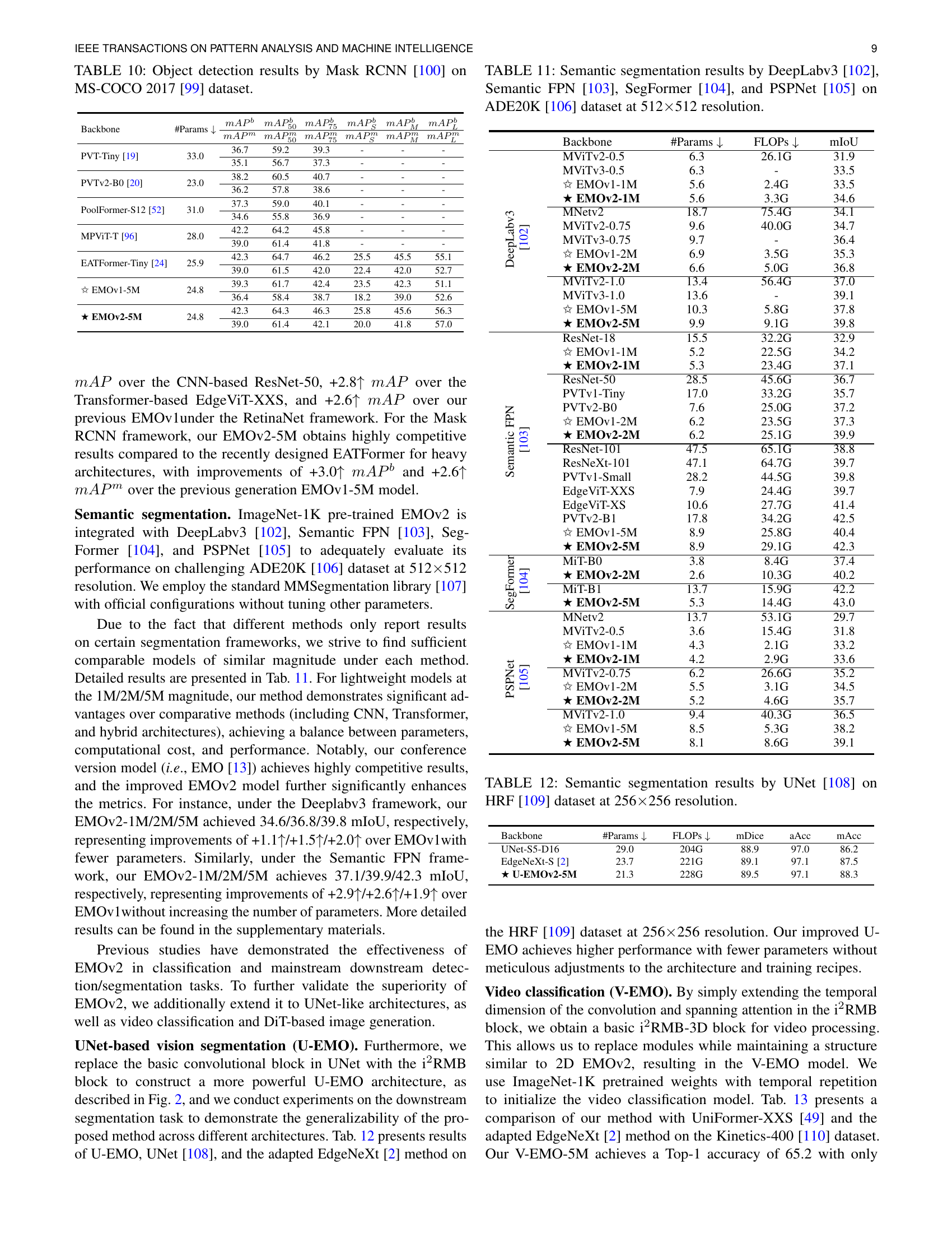
🔼 This table presents a comparison of semantic segmentation performance achieved by different models on the HRF dataset. Specifically, it shows the results obtained using the UNet architecture with various backbones on images with a resolution of 256x256 pixels. The metrics used to evaluate performance are likely mDice, average accuracy (aAcc), and mean accuracy (mAcc). The table aims to demonstrate how the choice of backbone network (and thus, the underlying model architecture) influences the overall performance of the UNet model for semantic segmentation. The focus is likely on the performance trade-off between the model’s size/complexity and its accuracy in the segmentation task.
read the caption
TABLE XII: Semantic segmentation results by UNet [108] on HRF [109] dataset at 256×\times×256 resolution.
| Backbone | #Params ↓ | FLOPs ↓ | mDice | aAcc | mAcc |
|---|---|---|---|---|---|
| UNet-S5-D16 | 29.0 | 204G | 88.9 | 97.0 | 86.2 |
| EdgeNeXt-S [2] | 23.7 | 221G | 89.1 | 97.1 | 87.5 |
| ★ U-EMOv2-5M | 21.3 | 228G | 89.5 | 97.1 | 88.3 |
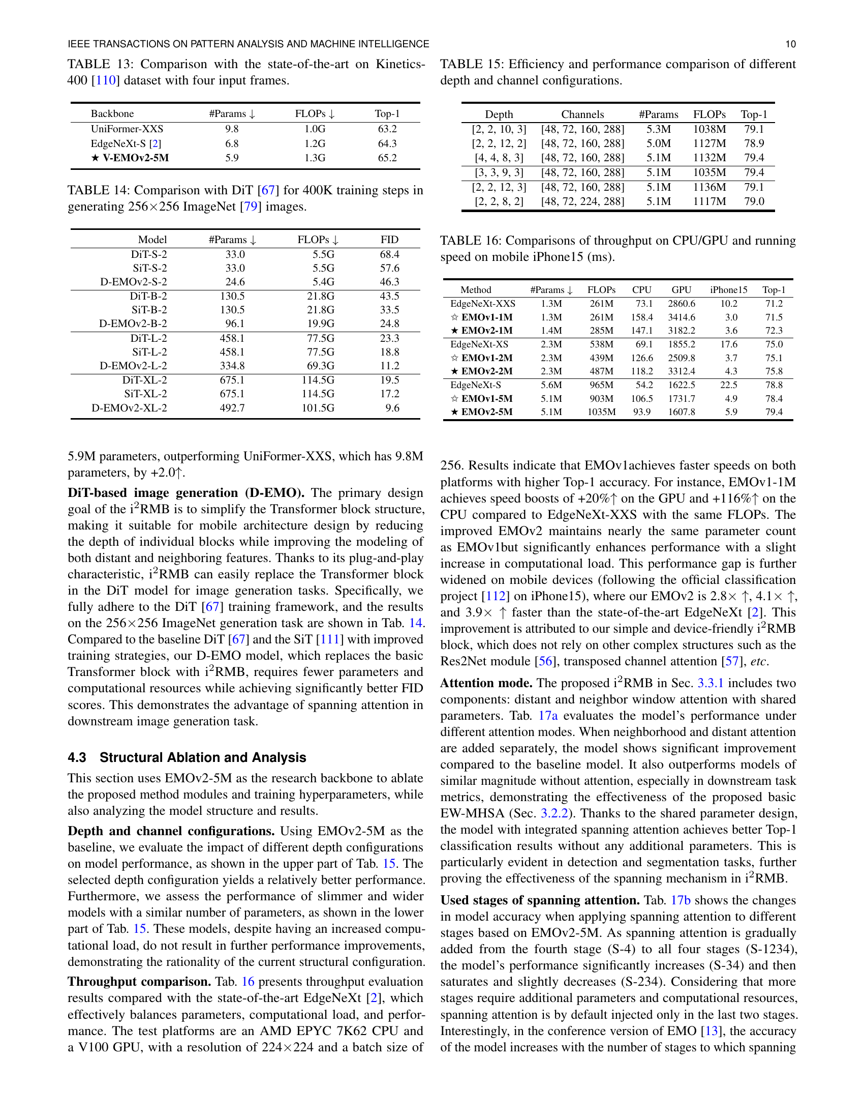
🔼 This table compares the performance of EMOv2-5M against other state-of-the-art models on the Kinetics-400 dataset, a benchmark for video recognition. The comparison focuses on top-1 accuracy, using four input frames for each video. It highlights EMOv2-5M’s performance relative to models with varying numbers of parameters and FLOPs (floating point operations). This helps illustrate the efficiency and accuracy of EMOv2-5M for video classification tasks.
read the caption
TABLE XIII: Comparison with the state-of-the-art on Kinetics-400 [110] dataset with four input frames.
| Backbone | #Params ↓ | FLOPs ↓ | Top-1 |
|---|---|---|---|
| UniFormer-XXS | 9.8 | 1.0G | 63.2 |
| EdgeNeXt-S [2] | 6.8 | 1.2G | 64.3 |
| ★ V-EMOv2-5M | 5.9 | 1.3G | 65.2 |
🔼 This table presents a comparison of the Fréchet Inception Distance (FID) scores achieved by different models when generating 256x256 ImageNet images after 400K training steps. It compares the performance of the proposed D-EMOv2 model against the baseline DiT model and its variations, showcasing the FID scores and the number of parameters and FLOPs used by each model.
read the caption
TABLE XIV: Comparison with DiT [67] for 400K training steps in generating 256×\times×256 ImageNet [79] images.
| Model | #Params ↓ | FLOPs ↓ | FID |
|---|---|---|---|
| DiT-S-2 | 33.0 | 5.5G | 68.4 |
| SiT-S-2 | 33.0 | 5.5G | 57.6 |
| D-EMOv2-S-2 | 24.6 | 5.4G | 46.3 |
| DiT-B-2 | 130.5 | 21.8G | 43.5 |
| SiT-B-2 | 130.5 | 21.8G | 33.5 |
| D-EMOv2-B-2 | 96.1 | 19.9G | 24.8 |
| DiT-L-2 | 458.1 | 77.5G | 23.3 |
| SiT-L-2 | 458.1 | 77.5G | 18.8 |
| D-EMOv2-L-2 | 334.8 | 69.3G | 11.2 |
| DiT-XL-2 | 675.1 | 114.5G | 19.5 |
| SiT-XL-2 | 675.1 | 114.5G | 17.2 |
| D-EMOv2-XL-2 | 492.7 | 101.5G | 9.6 |
🔼 This table presents a comparison of different model configurations, varying the depth and number of channels, while keeping the number of parameters relatively constant. It shows how these variations impact model efficiency (FLOPs) and performance (Top-1 accuracy). This helps to understand the optimal balance between depth, channel count, and overall model performance.
read the caption
TABLE XV: Efficiency and performance comparison of different depth and channel configurations.
| Depth | Channels | #Params | FLOPs | Top-1 |
|---|---|---|---|---|
| [2, 2, 10, 3] | [48, 72, 160, 288] | 5.3M | 1038M | 79.1 |
| [2, 2, 12, 2] | [48, 72, 160, 288] | 5.0M | 1127M | 78.9 |
| [4, 4, 8, 3] | [48, 72, 160, 288] | 5.1M | 1132M | 79.4 |
| [3, 3, 9, 3] | [48, 72, 160, 288] | 5.1M | 1035M | 79.4 |
| [2, 2, 12, 3] | [48, 72, 160, 288] | 5.1M | 1136M | 79.1 |
| [2, 2, 8, 2] | [48, 72, 224, 288] | 5.1M | 1117M | 79.0 |
🔼 This table compares the processing throughput (in images per second) of various models on CPU, GPU, and iPhone 15 mobile devices. It also shows the model’s running speed (in milliseconds) on an iPhone 15 and its Top-1 accuracy on the ImageNet-1K dataset. The models are categorized by parameter count, allowing comparison of performance across different model sizes.
read the caption
TABLE XVI: Comparisons of throughput on CPU/GPU and running speed on mobile iPhone15 (ms).
| Method | #Params ↓ | FLOPs | CPU | GPU | iPhone15 | Top-1 |
|---|---|---|---|---|---|---|
| EdgeNeXt-XXS | 1.3M | 261M | 73.1 | 2860.6 | 10.2 | 71.2 |
| ✩ EMOv1-1M | 1.3M | 261M | 158.4 | 3414.6 | 3.0 | 71.5 |
| ★ EMOv2-1M | 1.4M | 285M | 147.1 | 3182.2 | 3.6 | 72.3 |
| EdgeNeXt-XS | 2.3M | 538M | 69.1 | 1855.2 | 17.6 | 75.0 |
| ✩ EMOv1-2M | 2.3M | 439M | 126.6 | 2509.8 | 3.7 | 75.1 |
| ★ EMOv2-2M | 2.3M | 487M | 118.2 | 3312.4 | 4.3 | 75.8 |
| EdgeNeXt-S | 5.6M | 965M | 54.2 | 1622.5 | 22.5 | 78.8 |
| ✩ EMOv1-5M | 5.1M | 903M | 106.5 | 1731.7 | 4.9 | 78.4 |
| ★ EMOv2-5M | 5.1M | 1035M | 93.9 | 1607.8 | 5.9 | 79.4 |
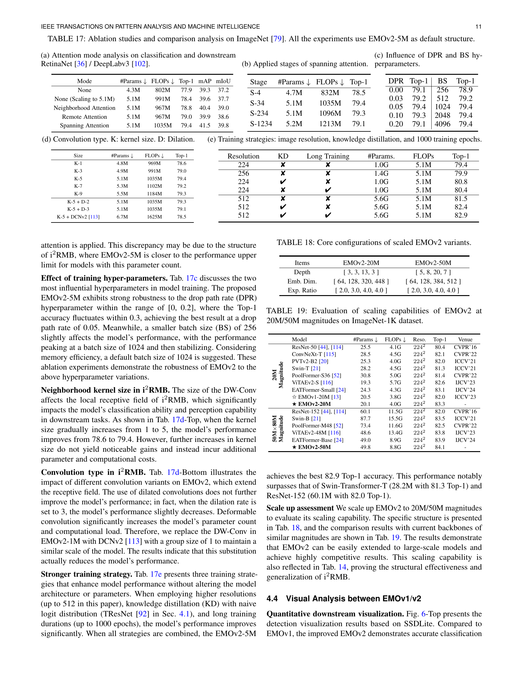
🔼 This table presents ablation study results and performance comparisons on the ImageNet dataset. Using the EMOv2-5M model as a baseline, various modifications and hyperparameter changes were tested, and their impacts on Top-1 accuracy, mean Average Precision (mAP) for object detection, and mean Intersection over Union (mIoU) for semantic segmentation are shown. The table allows for detailed analysis of the individual components’ contributions within the EMOv2 architecture and helps to assess the overall model’s robustness to different training strategies and design choices.
read the caption
TABLE XVII: Ablation studies and comparison analysis on ImageNet [79]. All the experiments use EMOv2-5M as default structure.
| Mode | #Params ↓ | FLOPs ↓ | Top-1 | mAP | mIoU |
|---|---|---|---|---|---|
| None | 4.3M | 802M | 77.9 | 39.3 | 37.2 |
| None (Scaling to 5.1M) | 5.1M | 991M | 78.4 | 39.6 | 37.7 |
| Neighborhood Attention | 5.1M | 967M | 78.8 | 40.4 | 39.0 |
| Remote Attention | 5.1M | 967M | 79.0 | 39.9 | 38.6 |
| Spanning Attention | 5.1M | 1035M | 79.4 | 41.5 | 39.8 |
🔼 This table details the core architectural configurations for scaled-up versions of the EMOv2 model. It shows how the depth, embedding dimension, and expansion ratio of the model’s building blocks change as the model’s size increases (from 5M to 20M and then 50M parameters). This allows for an analysis of the scalability and efficiency of the EMOv2 architecture.
read the caption
TABLE XVIII: Core configurations of scaled EMOv2 variants.
| Stage | #Params ↓ | FLOPs ↓ | Top-1 |
|---|---|---|---|
| S-4 | 4.7M | 832M | 78.5 |
| S-34 | 5.1M | 1035M | 79.4 |
| S-234 | 5.1M | 1096M | 79.3 |
| S-1234 | 5.2M | 1213M | 79.1 |
🔼 This table presents a comparison of the performance of EMOv2 models with 20 million and 50 million parameters on the ImageNet-1K dataset. It shows the number of parameters, FLOPs (floating point operations), resolution, and Top-1 accuracy for each model, along with a comparison to several other state-of-the-art models with similar parameter counts. This demonstrates the scalability of the EMOv2 architecture and its ability to maintain high accuracy even with a significant increase in model size.
read the caption
TABLE XIX: Evaluation of scaling capabilities of EMOv2 at 20M/50M magnitudes on ImageNet-1K dataset.
| DPR | Top-1 | BS | Top-1 |
|---|---|---|---|
| 0.00 | 79.1 | 256 | 78.9 |
| 0.03 | 79.2 | 512 | 79.2 |
| 0.05 | 79.4 | 1024 | 79.4 |
| 0.10 | 79.3 | 2048 | 79.4 |
| 0.20 | 79.1 | 4096 | 79.4 |
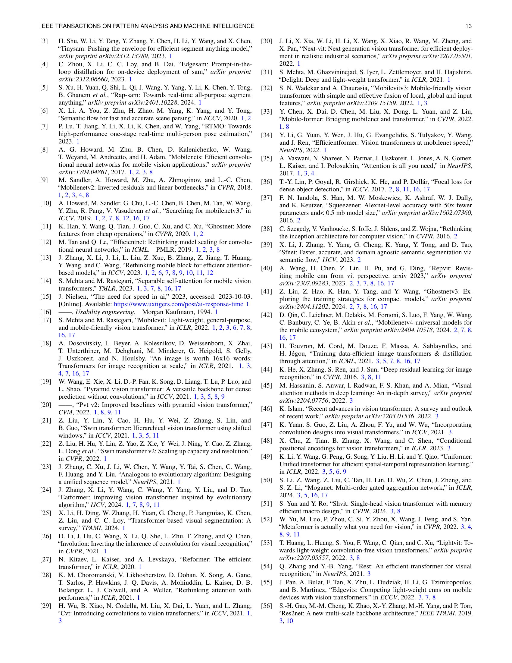
🔼 Table A1 compares the training hyperparameters used by various popular and contemporary lightweight vision models. It highlights the differences in training strategies employed by different models, offering insights into the methodologies used to train efficient vision models. This comparison focuses on key parameters such as the number of epochs, batch size, optimizer, learning rate and its decay schedule, use of warmup epochs, label smoothing, dropout, drop path rate, RandAugment, Mixup and Cutmix techniques, the use of erasing probability, the presence of positional embeddings, multi-scale samplers, the use of neural architecture search (NAS), knowledge distillation (KD), and re-parameterization strategies. The table’s goal is to showcase the diverse training regimes used in the field and to clearly state that the authors used a consistent, less intensive training approach for their own models, enabling more fair comparisons.
read the caption
TABLE A1: Comparison of training recipes among popular and contemporary methods and we employ the same setting in all experiments. Please zoom in for clearer comparisons. Abbreviations: MNet →→\rightarrow→ MobileNet; MViT →→\rightarrow→ MobileViT; EFormerv2 →→\rightarrow→ EfficientFormerv2; GNet →→\rightarrow→ GhostNet; NAS: Neural Architecture Search; KD: Knowledge Distillation; #Repre.: Re-parameterization strategy.
| Size | #Params ↓ | FLOPs ↓ | Top-1 |
|---|---|---|---|
| K-1 | 4.8M | 969M | 78.6 |
| K-3 | 4.9M | 991M | 79.0 |
| K-5 | 5.1M | 1035M | 79.4 |
| K-7 | 5.3M | 1102M | 79.2 |
| K-9 | 5.5M | 1184M | 79.3 |
| K-5 + D-2 | 5.1M | 1035M | 79.3 |
| K-5 + D-3 | 5.1M | 1035M | 79.1 |
| K-5 + DCNv2 [113] | 6.7M | 1625M | 78.5 |
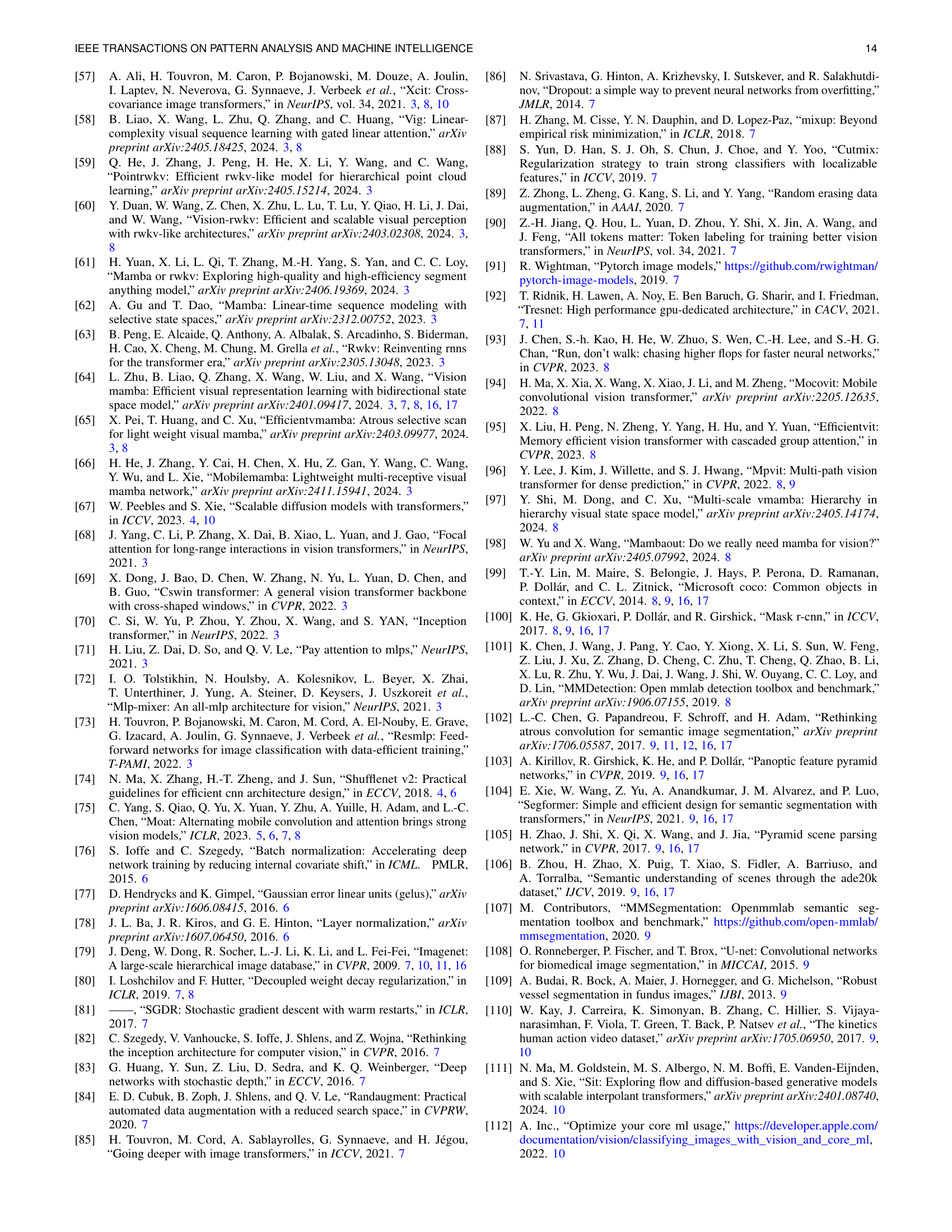
🔼 Table A2 presents a detailed comparison of object detection performance using two different models, SSDLite and RetinaNet, with our EMOv2 model on the MS-COCO 2017 dataset. The table shows the performance across different scales of the EMOv2 model (1M, 2M, 5M, 20M parameters), and includes results at both 320x320 and 512x512 image resolutions. The metrics used to evaluate the performance are mean Average Precision (mAP) for different object sizes (small, medium, large), as well as overall mAP. This allows for a comprehensive analysis of EMOv2’s effectiveness at different scales and resolutions in object detection tasks.
read the caption
TABLE A2: Detailed object detection performance using SSDLite [10] and RetinaNet [36] of our EMOv2 on MS-COCO 2017 [99] dataset. ††\dagger†: 512 ×\times× 512 resolution.
| Resolution | KD | Long Training | #Params. | FLOPs | Top-1 |
|---|---|---|---|---|---|
| 224 | ✘ | ✘ | 1.0G | 5.1M | 79.4 |
| 256 | ✘ | ✘ | 1.4G | 5.1M | 79.9 |
| 224 | ✔ | ✘ | 1.0G | 5.1M | 80.8 |
| 224 | ✘ | ✔ | 1.0G | 5.1M | 80.4 |
| 512 | ✘ | ✘ | 5.6G | 5.1M | 81.5 |
| 512 | ✔ | ✘ | 5.6G | 5.1M | 82.4 |
| 512 | ✔ | ✔ | 5.6G | 5.1M | 82.9 |
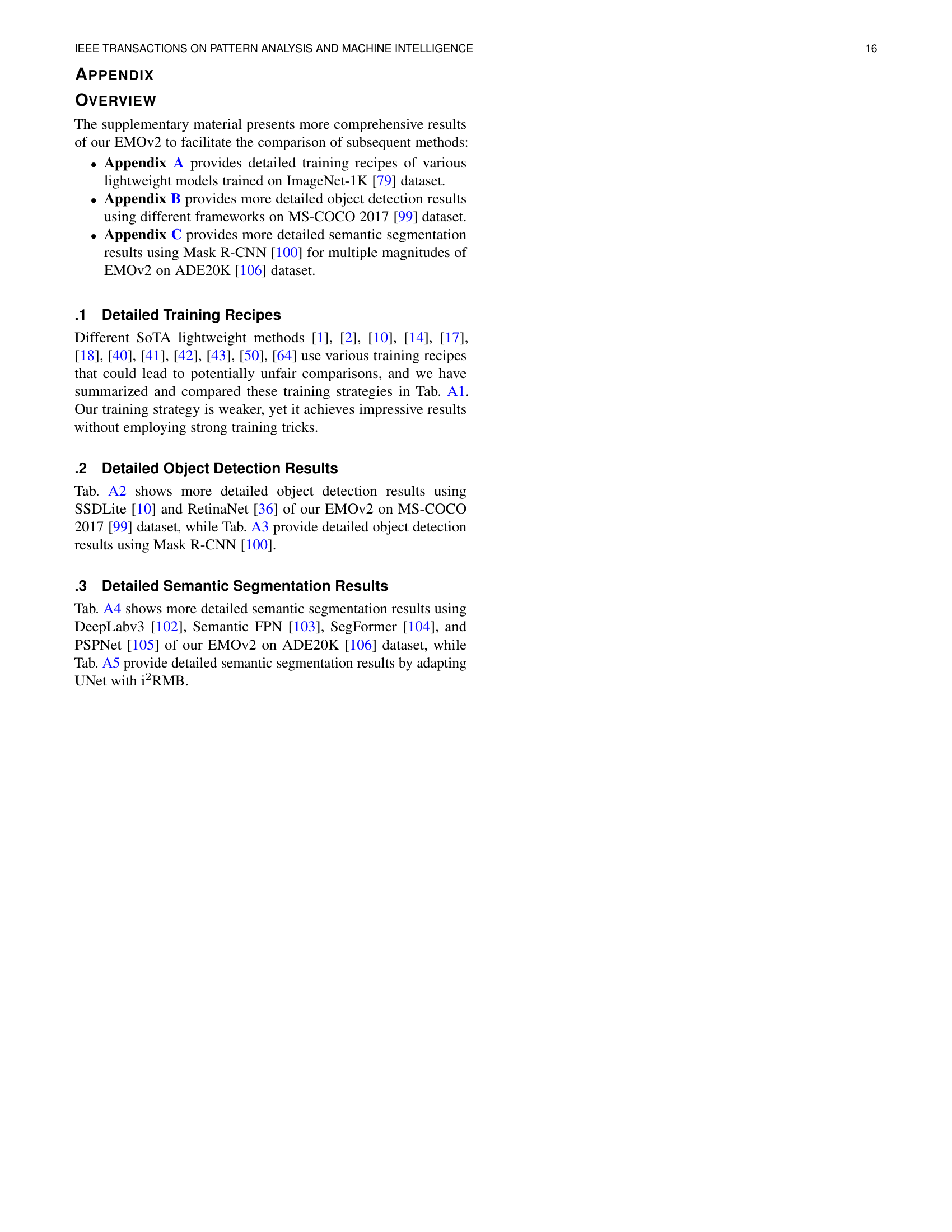
🔼 Table A3 presents a detailed analysis of object detection performance using the Mask RCNN model. It showcases the results obtained by employing different versions of the EMOv2 model (with varying numbers of parameters) on the MS-COCO 2017 dataset. The table provides a comprehensive evaluation, breaking down the performance across different metrics, allowing for a thorough comparison of the EMOv2 model’s effectiveness in object detection compared to other state-of-the-art models.
read the caption
TABLE A3: Detailed object detection performance using Mask RCNN [100] of our EMOv2 on MS-COCO 2017 [99] dataset.
| Items | EMOV2-20M | EMOV2-50M |
|---|---|---|
| Depth | [ 3, 3, 13, 3 ] | [ 5, 8, 20, 7 ] |
| Emb. Dim. | [ 64, 128, 320, 448 ] | [ 64, 128, 384, 512 ] |
| Exp. Ratio | [ 2.0, 3.0, 4.0, 4.0 ] | [ 2.0, 3.0, 4.0, 4.0 ] |
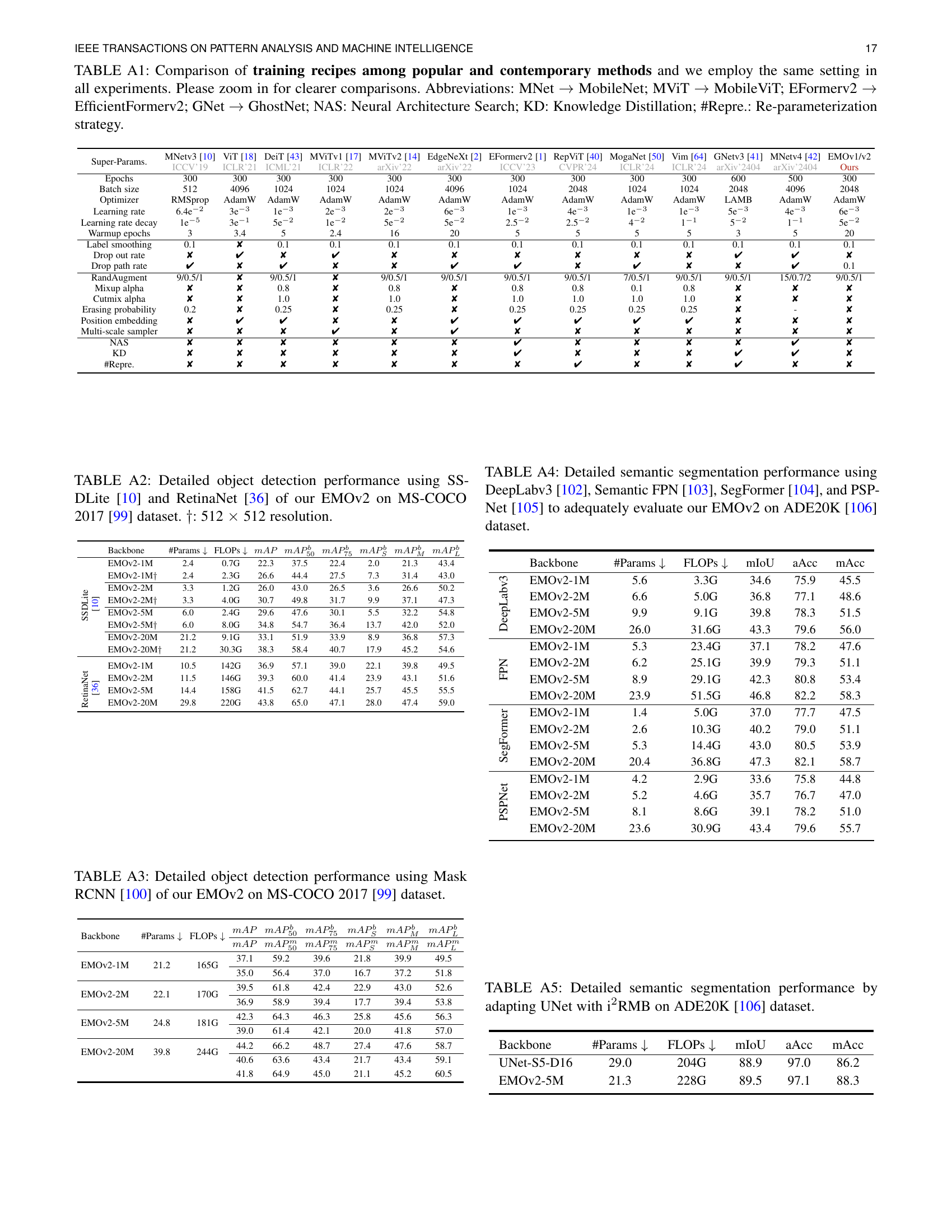
🔼 Table A4 presents a detailed comparison of semantic segmentation performance achieved by different models on the ADE20K dataset. It assesses the models’ effectiveness using four popular semantic segmentation architectures: DeepLabv3, Semantic FPN, SegFormer, and PSPNet. The table focuses on demonstrating the performance of various sizes of the EMOv2 model (1M, 2M, 5M, and 20M parameters), highlighting its effectiveness across different scales. The results include mIoU, aAcc, and mAcc, offering a comprehensive evaluation of the EMOv2’s capabilities in semantic segmentation.
read the caption
TABLE A4: Detailed semantic segmentation performance using DeepLabv3 [102], Semantic FPN [103], SegFormer [104], and PSPNet [105] to adequately evaluate our EMOv2 on ADE20K [106] dataset.
| Model | #Params ↓ | FLOPs ↓ | Reso. | Top-1 | Venue |
|---|---|---|---|---|---|
| ResNet-50 [44, 114] | 25.5M | 4.1G | 2242 | 80.4 | CVPR’16 |
| ConvNeXt-T [115] | 28.5M | 4.5G | 2242 | 82.1 | CVPR’22 |
| PVTv2-B2 [20] | 25.3M | 4.0G | 2242 | 82.0 | ICCV’21 |
| Swin-T [21] | 28.2M | 4.5G | 2242 | 81.3 | ICCV’21 |
| PoolFormer-S36 [52] | 30.8M | 5.0G | 2242 | 81.4 | CVPR’22 |
| ViTAEv2-S [116] | 19.3M | 5.7G | 2242 | 82.6 | IJCV’23 |
| EATFormer-Small [24] | 24.3M | 4.3G | 2242 | 83.1 | IJCV’24 |
| ✩ EMOV1-20M [13] | 20.5M | 3.8G | 2242 | 82.0 | ICCV’23 |
| ★ EMOV2-20M | 20.1M | 4.0G | 2242 | 83.3 | - |
| ResNet-152 [44, 114] | 60.1M | 11.5G | 2242 | 82.0 | CVPR’16 |
| Swin-B [21] | 87.7M | 15.5G | 2242 | 83.5 | ICCV’21 |
| PoolFormer-M48 [52] | 73.4M | 11.6G | 2242 | 82.5 | CVPR’22 |
| ViTAEv2-48M [116] | 48.6M | 13.4G | 2242 | 83.8 | IJCV’23 |
| EATFormer-Base [24] | 49.0M | 8.9G | 2242 | 83.9 | IJCV’24 |
| ★ EMOV2-50M | 49.8M | 8.8G | 2242 | 84.1 | - |
🔼 Table A5 presents a detailed comparison of semantic segmentation performance achieved using different models on the ADE20K dataset. The table specifically focuses on the results obtained by adapting the UNet architecture with the Improved Inverted Residual Mobile Block (i2RMB) introduced in the paper. It shows how incorporating i2RMB impacts the model’s performance metrics like mIoU, average accuracy (aAcc), and mean accuracy (mAcc). The comparison includes a baseline UNet model and the modified UNet with the i2RMB, offering insights into the effectiveness of i2RMB for semantic segmentation tasks.
read the caption
TABLE A5: Detailed semantic segmentation performance by adapting UNet with i2RMB on ADE20K [106] dataset.
Full paper#
