↗ arXiv ↗ Hugging Face ↗ Papers with Code
TL;DR#
Image super-resolution (SR) aims to enhance low-resolution images. Existing diffusion model-based SR methods often involve complex optimization or fine-tuning, limiting efficiency and flexibility. Furthermore, fixed sampling steps hinder adaptability to diverse degradation types.
This paper introduces InvSR, a novel SR technique based on diffusion inversion. Instead of modifying the diffusion network, InvSR uses a deep noise predictor to estimate optimal noise maps, initializing the sampling process and generating high-resolution images. This approach allows for arbitrary sampling steps, providing great flexibility and efficiency, making it suitable for various degradation types. InvSR shows competitive or superior performance to existing methods, even with a single sampling step.
Key Takeaways#
Why does it matter?#
This paper is important because it presents a novel and efficient approach to image super-resolution using diffusion models. It addresses the limitations of existing methods by offering flexible and arbitrary-step sampling, leading to improved efficiency and adaptability. This work is highly relevant to current research trends in image generation and restoration and opens new avenues for developing more versatile and practical super-resolution techniques.
Visual Insights#

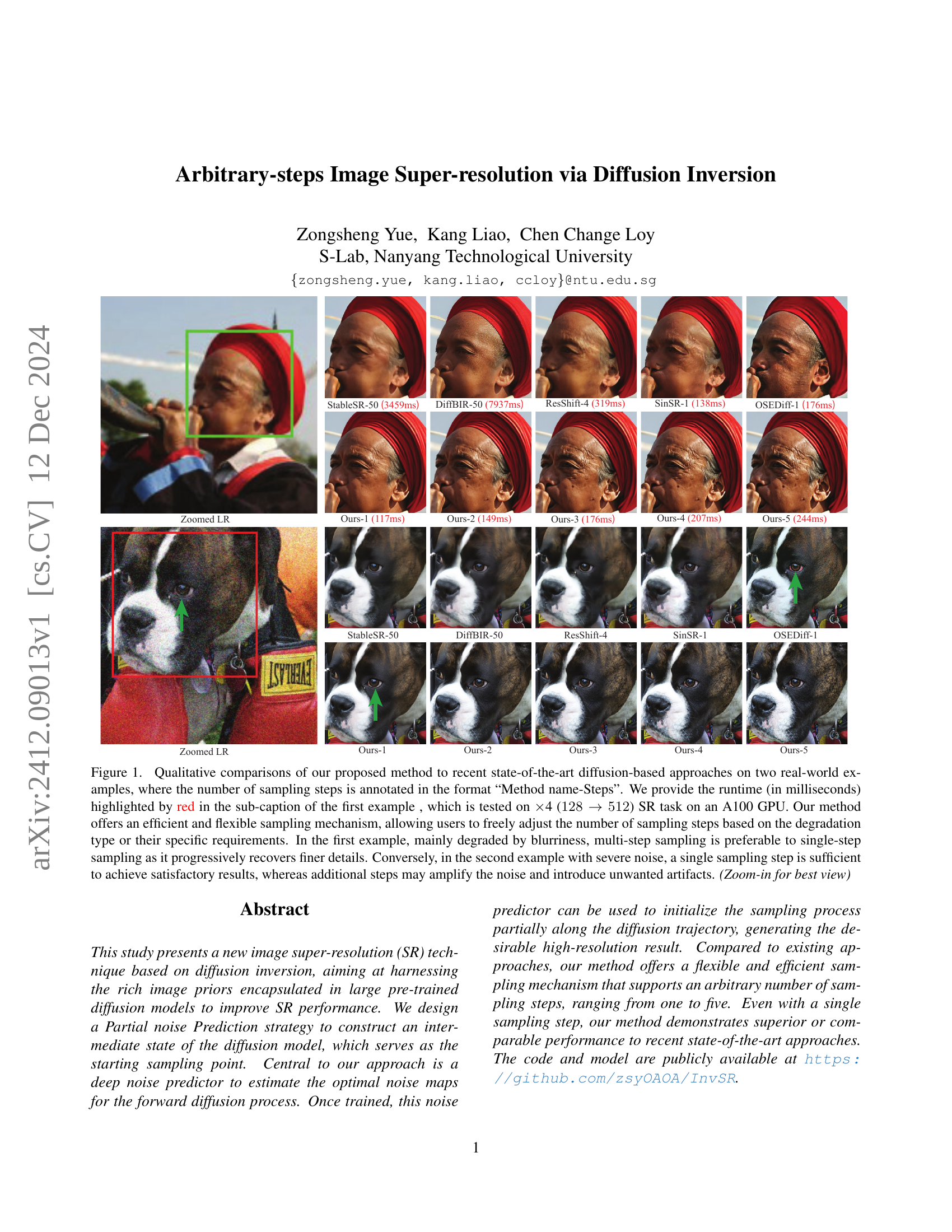
🔼 This figure showcases a comparison between the proposed image super-resolution (SR) method and other state-of-the-art diffusion-based SR methods. Two real-world examples are used for the comparison. The number of sampling steps used for each method is indicated. The first example demonstrates that for blurry images, multiple sampling steps progressively improve the result with finer details. The second example, however, shows that a single sampling step is preferable for images with noise as additional steps may exacerbate it. Runtimes for the various methods on an A100 GPU are shown for the first example’s x4 (128 to 512 pixels) super-resolution task. The proposed method is highlighted as offering a flexible and efficient sampling process that can be adjusted according to the image’s degradation.
read the caption
Figure 1: Qualitative comparisons of our proposed method to recent state-of-the-art diffusion-based approaches on two real-world examples, where the number of sampling steps is annotated in the format “Method name-Steps”. We provide the runtime (in milliseconds) highlighted by red in the sub-caption of the first example , which is tested on ×\times×4 (128→512→128512128\rightarrow 512128 → 512) SR task on an A100 GPU. Our method offers an efficient and flexible sampling mechanism, allowing users to freely adjust the number of sampling steps based on the degradation type or their specific requirements. In the first example, mainly degraded by blurriness, multi-step sampling is preferable to single-step sampling as it progressively recovers finer details. Conversely, in the second example with severe noise, a single sampling step is sufficient to achieve satisfactory results, whereas additional steps may amplify the noise and introduce unwanted artifacts. (Zoom-in for best view)
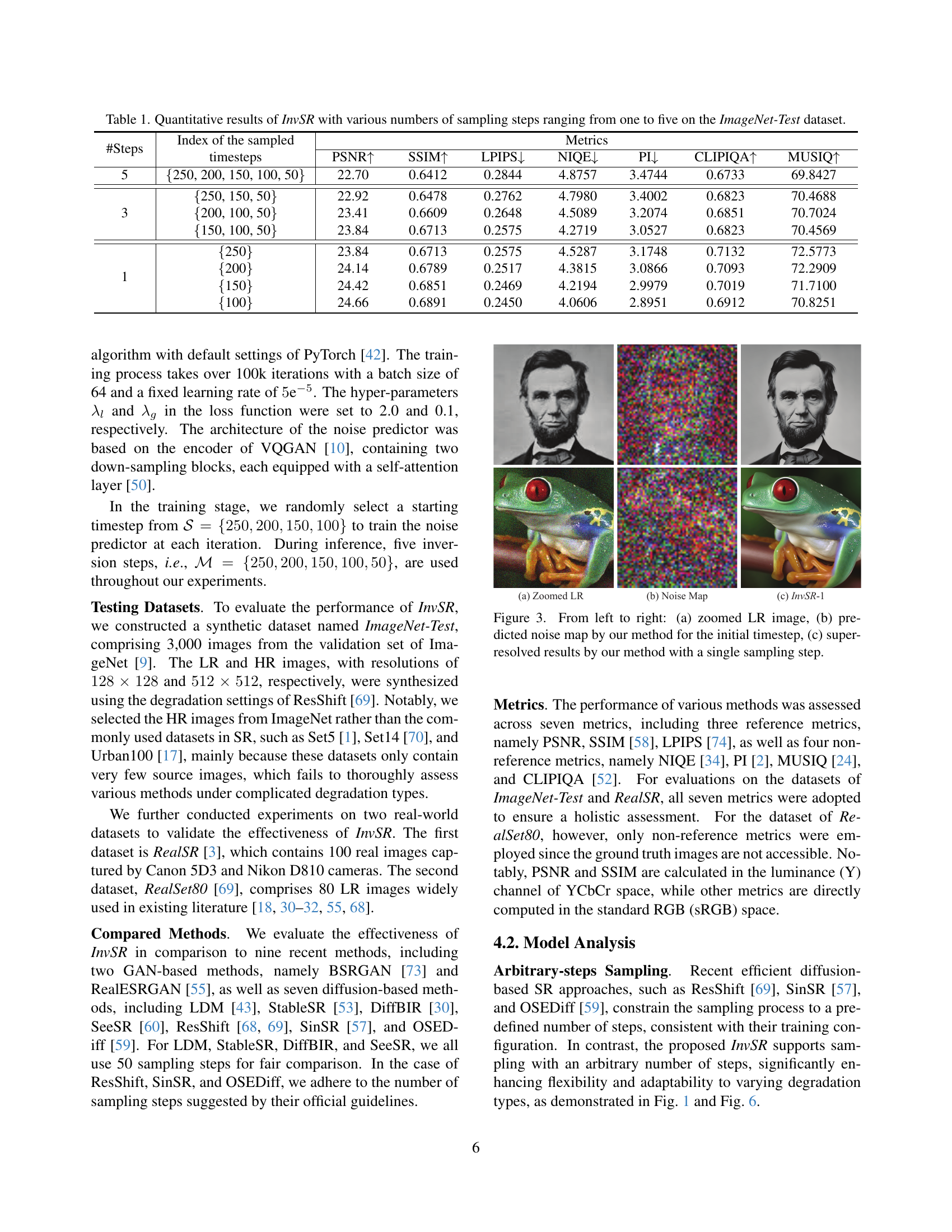
| #Steps | Index of the sampled timesteps | PSNR ↑ | SSIM ↑ | LPIPS ↓ | NIQE ↓ | PI ↓ | CLIPIQA ↑ | MUSIQ ↑ |
|---|---|---|---|---|---|---|---|---|
| 9 | ||||||||
| 5 | {250, 200, 150, 100, 50} | 22.70 | 0.6412 | 0.2844 | 4.8757 | 3.4744 | 0.6733 | 69.8427 |
| 3 | {250, 150, 50} | 22.92 | 0.6478 | 0.2762 | 4.7980 | 3.4002 | 0.6823 | 70.4688 |
| {200, 100, 50} | 23.41 | 0.6609 | 0.2648 | 4.5089 | 3.2074 | 0.6851 | 70.7024 | |
| {150, 100, 50} | 23.84 | 0.6713 | 0.2575 | 4.2719 | 3.0527 | 0.6823 | 70.4569 | |
| 1 | {250} | 23.84 | 0.6713 | 0.2575 | 4.5287 | 3.1748 | 0.7132 | 72.5773 |
| {200} | 24.14 | 0.6789 | 0.2517 | 4.3815 | 3.0866 | 0.7093 | 72.2909 | |
| {150} | 24.42 | 0.6851 | 0.2469 | 4.2194 | 2.9979 | 0.7019 | 71.7100 | |
| {100} | 24.66 | 0.6891 | 0.2450 | 4.0606 | 2.8951 | 0.6912 | 70.8251 |
🔼 This table presents a quantitative evaluation of the proposed InvSR (Arbitrary-steps Image Super-resolution via Diffusion Inversion) method. It shows the performance of InvSR across different numbers of sampling steps (1, 3, 5) on the ImageNet-Test dataset. For each sampling step configuration, the results are reported for several different subsets of timesteps used during the sampling process. The metrics used to evaluate InvSR include Peak Signal-to-Noise Ratio (PSNR), Structural Similarity Index (SSIM), Learned Perceptual Image Patch Similarity (LPIPS), Natural Image Quality Evaluator (NIQE), Perceptual Index (PI), CLIP-based Image Quality Assessment (CLIPIQA), and Multi-Scale Image Quality (MUSIQ). Higher values for PSNR, SSIM, CLIPIQA, and MUSIQ indicate better performance, while lower values for LPIPS and NIQE are preferable. This allows for a comprehensive analysis of InvSR’s performance under different sampling strategies and provides insights into the trade-off between computational cost and image quality.
read the caption
Table 1: Quantitative results of InvSR with various numbers of sampling steps ranging from one to five on the ImageNet-Test dataset.
In-depth insights#
Diffusion Inversion SR#
Diffusion Inversion for Super-Resolution (SR) leverages the power of pre-trained diffusion models to overcome the ill-posed nature of SR. Unlike methods modifying the diffusion model itself, diffusion inversion aims to find the optimal noise map that, when fed into the pre-trained model, generates the high-resolution (HR) image from a low-resolution (LR) input. This approach maximizes the utilization of the existing diffusion model’s rich image priors. A key challenge is the computational cost of calculating noise maps for many diffusion steps. To address this, the technique of partial noise prediction is introduced. This cleverly reduces the computational load by focusing on predicting only the starting noise map, significantly improving efficiency. The method demonstrates flexibility by allowing for varying numbers of sampling steps, adapting to different degradation types and offering a trade-off between computational speed and reconstruction fidelity. This adaptability makes it superior to methods relying on fixed sampling steps. Overall, diffusion inversion offers a promising and efficient path towards high-fidelity SR, particularly by capitalizing on readily available, powerful pre-trained diffusion models.
Partial Noise Prediction#
The concept of “Partial Noise Prediction” in the context of image super-resolution via diffusion inversion is a key innovation that addresses computational complexity. Traditional diffusion-based SR methods often involve predicting noise maps for every step of the diffusion process, making them computationally expensive. Partial Noise Prediction cleverly bypasses this by focusing on predicting noise maps only for an intermediate state of the diffusion process, a point chosen strategically for an optimal balance between fidelity and efficiency. This is motivated by the observation that low-resolution (LR) images differ from high-resolution (HR) images primarily in high-frequency details. The intermediate state acts as a shortcut in the inversion trajectory, enabling the use of fewer steps in generating the HR image while maintaining a satisfactory quality. The effectiveness of this method relies on a well-trained noise predictor that can accurately estimate the optimal noise maps for initializing the sampling process, therefore requiring high-quality training data. This approach greatly reduces computational cost without significantly sacrificing the quality of the super-resolved images, making it a more practical solution for real-world applications. The flexibility to choose from several pre-defined starting points also makes the method robust to different degradation types.
Arbitrary Steps Sampling#
The concept of “Arbitrary Steps Sampling” in image super-resolution (SR) using diffusion models offers a significant advantage over traditional fixed-step methods. Flexibility is key; it allows the model to adapt the number of sampling steps to the specific characteristics of the input image and its degradation type. This contrasts with fixed-step approaches that often struggle with varying degradation levels, leading to suboptimal results. Efficiency is another major benefit, as fewer steps are needed for less complex images, saving computation time. The ability to adjust the number of steps based on image quality is crucial, as it allows for optimal balance between detail recovery and noise amplification. For instance, blurry images might benefit from multiple steps to recover fine details, while noisy images might be best served by a single step to avoid noise amplification. This adaptability is a crucial step towards creating more robust and efficient SR models that generalize well across diverse real-world scenarios.
InvSR Efficiency Analysis#
An InvSR efficiency analysis would reveal crucial insights into its computational cost. Speed is paramount; comparing InvSR’s inference time to existing SR methods (GAN-based, diffusion-based) is key. A breakdown of runtime components (noise prediction, sampling steps) would highlight bottlenecks. Memory usage is another critical factor, especially for high-resolution images. Analyzing memory allocation during each stage (noise estimation, diffusion process) is vital. Parameter count should also be considered; a smaller model size translates to faster processing and lower resource demands. Scalability should be assessed: does performance degrade significantly with increasing image size or complexity? Finally, an analysis should explore hardware acceleration opportunities (GPU utilization, optimized kernels) to minimize the execution time, potentially revealing further improvements.
Future Research Scope#
Future research could explore improving the efficiency of the noise predictor by employing more lightweight network architectures or more efficient training strategies. Investigating alternative sampling algorithms beyond those currently used, potentially incorporating techniques from other generative models, is crucial for further enhancing efficiency and flexibility. A key area for future work involves handling diverse degradation types more effectively. While this paper addresses blur and noise, a more robust method capable of adapting to diverse and complex real-world degradations is needed. Finally, the exploration of different diffusion models and their effect on SR performance warrants further investigation, including testing on models beyond Stable Diffusion to assess the approach’s generalizability and potentially improving quality and efficiency.
More visual insights#
More on figures

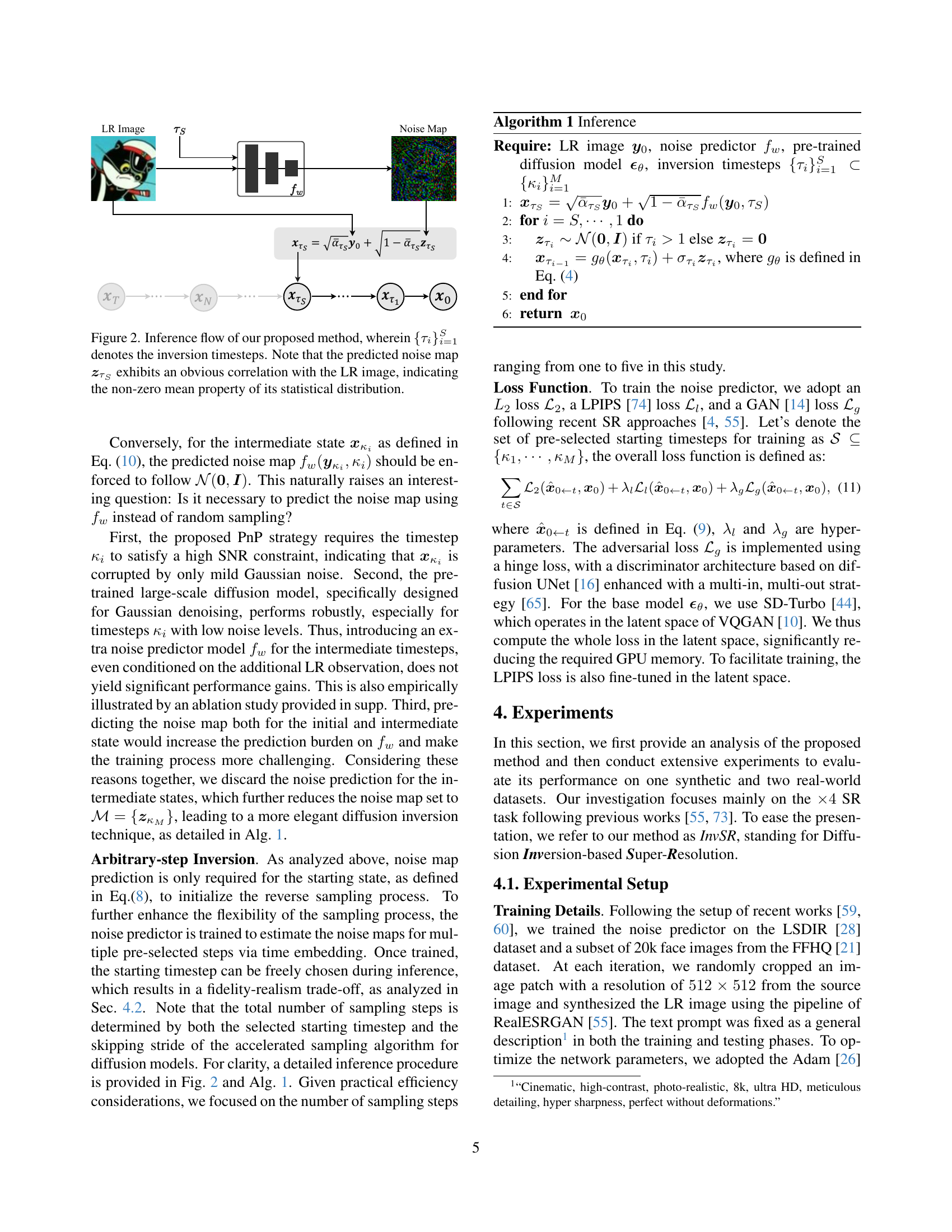
🔼 Figure 2 illustrates the inference process of the proposed image super-resolution method. The input is a low-resolution (LR) image. A noise predictor network (fw) estimates the initial noise map (zτS) needed to start the reverse diffusion process. This initial noise map is added to a scaled version of the LR image, creating the starting point for the sampling process. The reverse diffusion process, using a pre-trained diffusion model, then iteratively refines this initial estimate to generate the final high-resolution (HR) image. The figure highlights that the predicted initial noise map (zτS) shows a strong correlation with the input LR image, exhibiting a non-zero mean in its statistical distribution, which is unusual for typical diffusion processes.
read the caption
Figure 2: Inference flow of our proposed method, wherein {τi}i=1Ssuperscriptsubscriptsubscript𝜏𝑖𝑖1𝑆\{\tau_{i}\}_{i=1}^{S}{ italic_τ start_POSTSUBSCRIPT italic_i end_POSTSUBSCRIPT } start_POSTSUBSCRIPT italic_i = 1 end_POSTSUBSCRIPT start_POSTSUPERSCRIPT italic_S end_POSTSUPERSCRIPT denotes the inversion timesteps. Note that the predicted noise map 𝒛τSsubscript𝒛subscript𝜏𝑆\bm{z}_{\tau_{S}}bold_italic_z start_POSTSUBSCRIPT italic_τ start_POSTSUBSCRIPT italic_S end_POSTSUBSCRIPT end_POSTSUBSCRIPT exhibits an obvious correlation with the LR image, indicating the non-zero mean property of its statistical distribution.

🔼 This figure visually demonstrates the core concept of the proposed method. It shows three images: (a) a zoomed-in view of a low-resolution (LR) image used as input; (b) the noise map predicted by the model’s noise predictor network for the initial step of the diffusion process; and (c) the final super-resolved high-resolution (HR) image produced by the method using only a single sampling step of the reverse diffusion process. The predicted noise map highlights the model’s ability to estimate the optimal noise needed to initiate the upscaling process within the diffusion model, leading directly to a high-resolution result in a single step. This illustrates the efficiency and efficacy of the proposed Partial Noise Prediction (PnP) strategy.
read the caption
Figure 3: From left to right: (a) zoomed LR image, (b) predicted noise map by our method for the initial timestep, (c) super-resolved results by our method with a single sampling step.

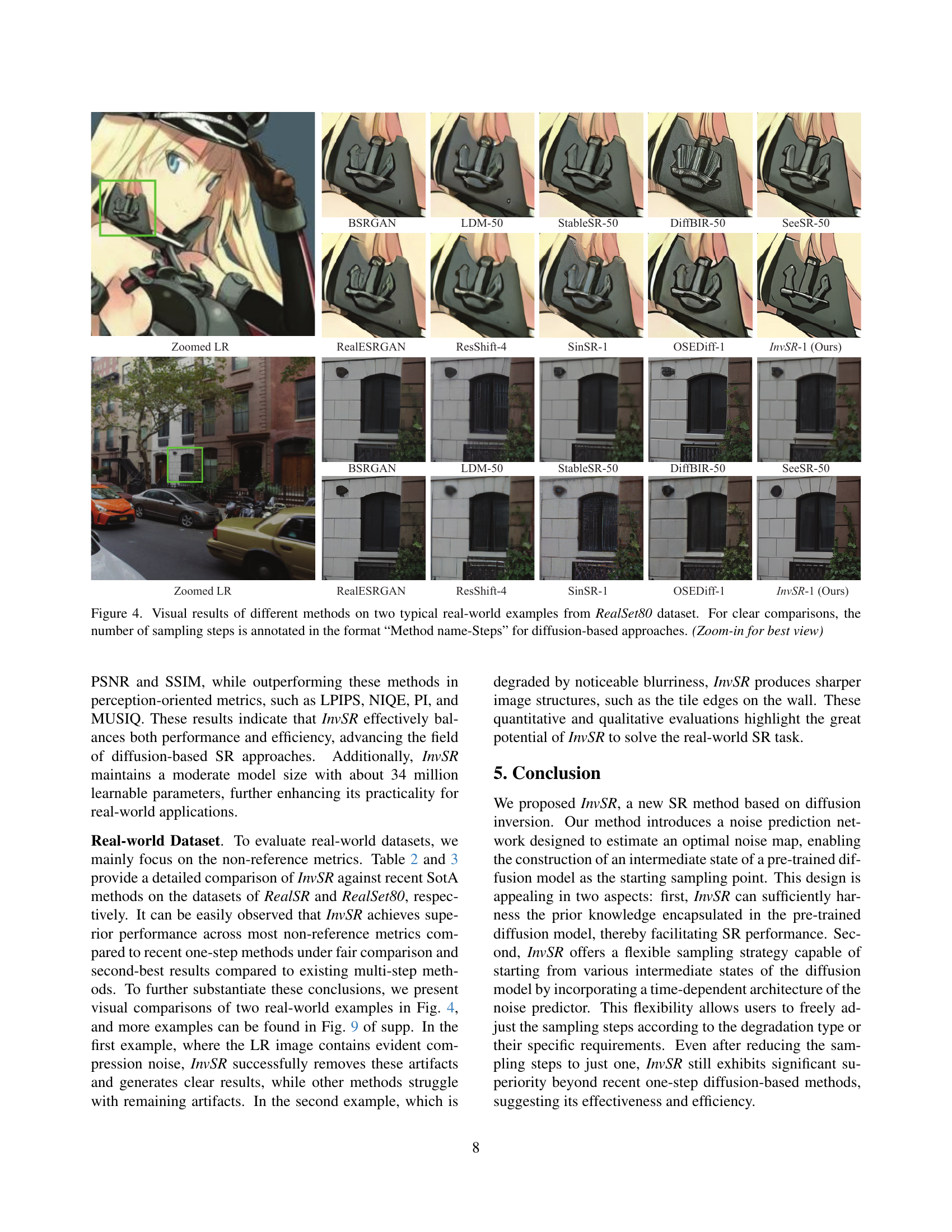
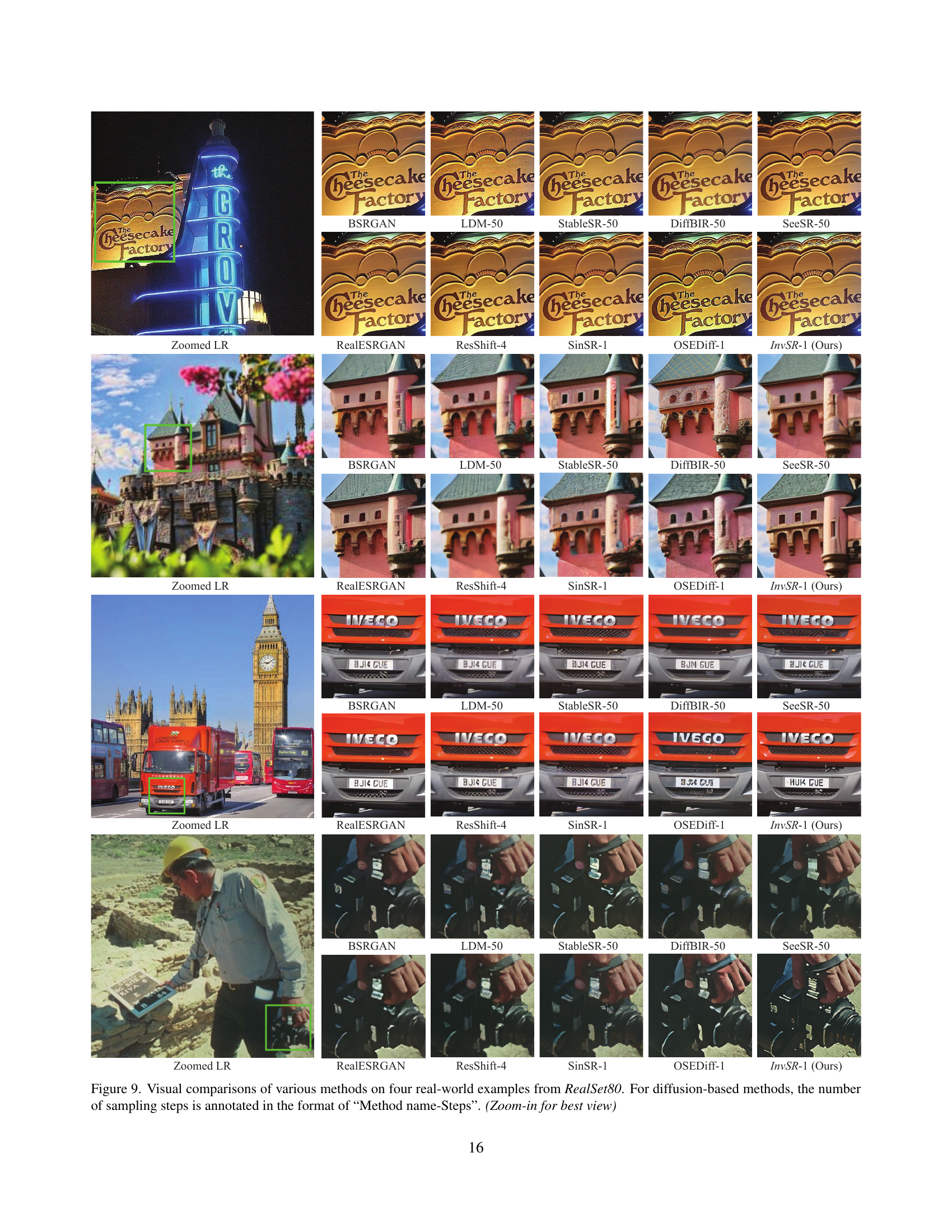
🔼 Figure 4 presents a visual comparison of different image super-resolution (SR) methods applied to two real-world examples from the RealSet80 dataset. The images showcase the performance of various techniques, including both diffusion-based and non-diffusion-based approaches. For the diffusion-based SR methods, the number of sampling steps used during the process is clearly indicated within the image caption, following the format ‘Method Name-Steps.’ This allows for an easy and direct comparison of performance at varying numbers of steps. The images are intended to be viewed at a zoomed-in level to fully appreciate the fine-grained details of the results.
read the caption
Figure 4: Visual results of different methods on two typical real-world examples from RealSet80 dataset. For clear comparisons, the number of sampling steps is annotated in the format “Method name-Steps” for diffusion-based approaches. (Zoom-in for best view)

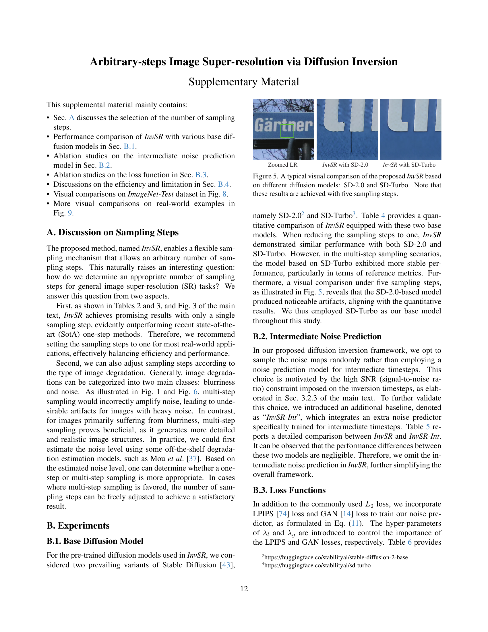
🔼 This figure compares the performance of the proposed InvSR method using two different pre-trained diffusion models as its base: Stable Diffusion 2.0 (SD-2.0) and Stable Diffusion Turbo (SD-Turbo). Both versions of InvSR utilize five sampling steps in the image generation process. The visual comparison allows for a qualitative assessment of the image quality and the differences in the generated results when using different base diffusion models. This helps to demonstrate the impact of the choice of base diffusion model on the final image quality produced by InvSR.
read the caption
Figure 5: A typical visual comparison of the proposed InvSR based on different diffusion models: SD-2.0 and SD-Turbo. Note that these results are achieved with five sampling steps.

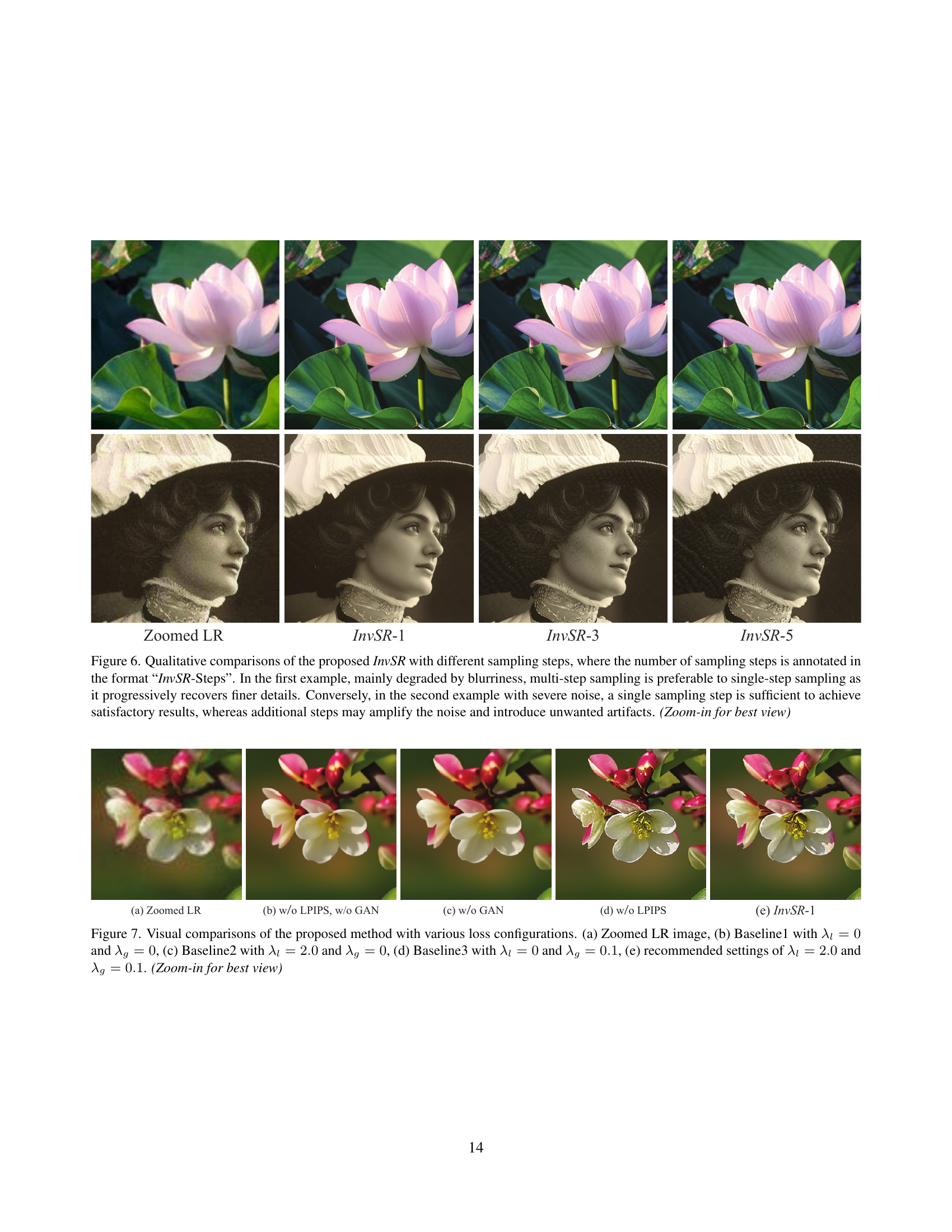
🔼 Figure 6 presents a qualitative comparison of the InvSR model’s performance using different numbers of sampling steps. The number of steps used is indicated as ‘InvSR-Steps’. The top row shows an image primarily affected by blur. Here, multiple sampling steps are superior to a single step because they progressively reveal finer details, enhancing the image quality. In contrast, the bottom row illustrates an image with significant noise. In this case, a single sampling step is ideal; additional steps would intensify the noise and introduce undesirable artifacts. The ‘Zoom-in for best view’ note suggests the details are best observed at a higher magnification.
read the caption
Figure 6: Qualitative comparisons of the proposed InvSR with different sampling steps, where the number of sampling steps is annotated in the format “InvSR-Steps”. In the first example, mainly degraded by blurriness, multi-step sampling is preferable to single-step sampling as it progressively recovers finer details. Conversely, in the second example with severe noise, a single sampling step is sufficient to achieve satisfactory results, whereas additional steps may amplify the noise and introduce unwanted artifacts. (Zoom-in for best view)

🔼 This figure shows the impact of different loss function configurations on the performance of the proposed image super-resolution method. It compares the results of using only the L2 loss (Baseline1), adding the LPIPS loss (Baseline2), adding the GAN loss (Baseline3), and finally using the recommended combination of L2, LPIPS, and GAN losses (InvSR-1). The zoomed LR image is also provided for comparison. The goal is to illustrate how the different loss functions affect the visual quality of the super-resolved image.
read the caption
Figure 7: Visual comparisons of the proposed method with various loss configurations. (a) Zoomed LR image, (b) Baseline1 with λl=0subscript𝜆𝑙0\lambda_{l}=0italic_λ start_POSTSUBSCRIPT italic_l end_POSTSUBSCRIPT = 0 and λg=0subscript𝜆𝑔0\lambda_{g}=0italic_λ start_POSTSUBSCRIPT italic_g end_POSTSUBSCRIPT = 0, (c) Baseline2 with λl=2.0subscript𝜆𝑙2.0\lambda_{l}=2.0italic_λ start_POSTSUBSCRIPT italic_l end_POSTSUBSCRIPT = 2.0 and λg=0subscript𝜆𝑔0\lambda_{g}=0italic_λ start_POSTSUBSCRIPT italic_g end_POSTSUBSCRIPT = 0, (d) Baseline3 with λl=0subscript𝜆𝑙0\lambda_{l}=0italic_λ start_POSTSUBSCRIPT italic_l end_POSTSUBSCRIPT = 0 and λg=0.1subscript𝜆𝑔0.1\lambda_{g}=0.1italic_λ start_POSTSUBSCRIPT italic_g end_POSTSUBSCRIPT = 0.1, (e) recommended settings of λl=2.0subscript𝜆𝑙2.0\lambda_{l}=2.0italic_λ start_POSTSUBSCRIPT italic_l end_POSTSUBSCRIPT = 2.0 and λg=0.1subscript𝜆𝑔0.1\lambda_{g}=0.1italic_λ start_POSTSUBSCRIPT italic_g end_POSTSUBSCRIPT = 0.1. (Zoom-in for best view)

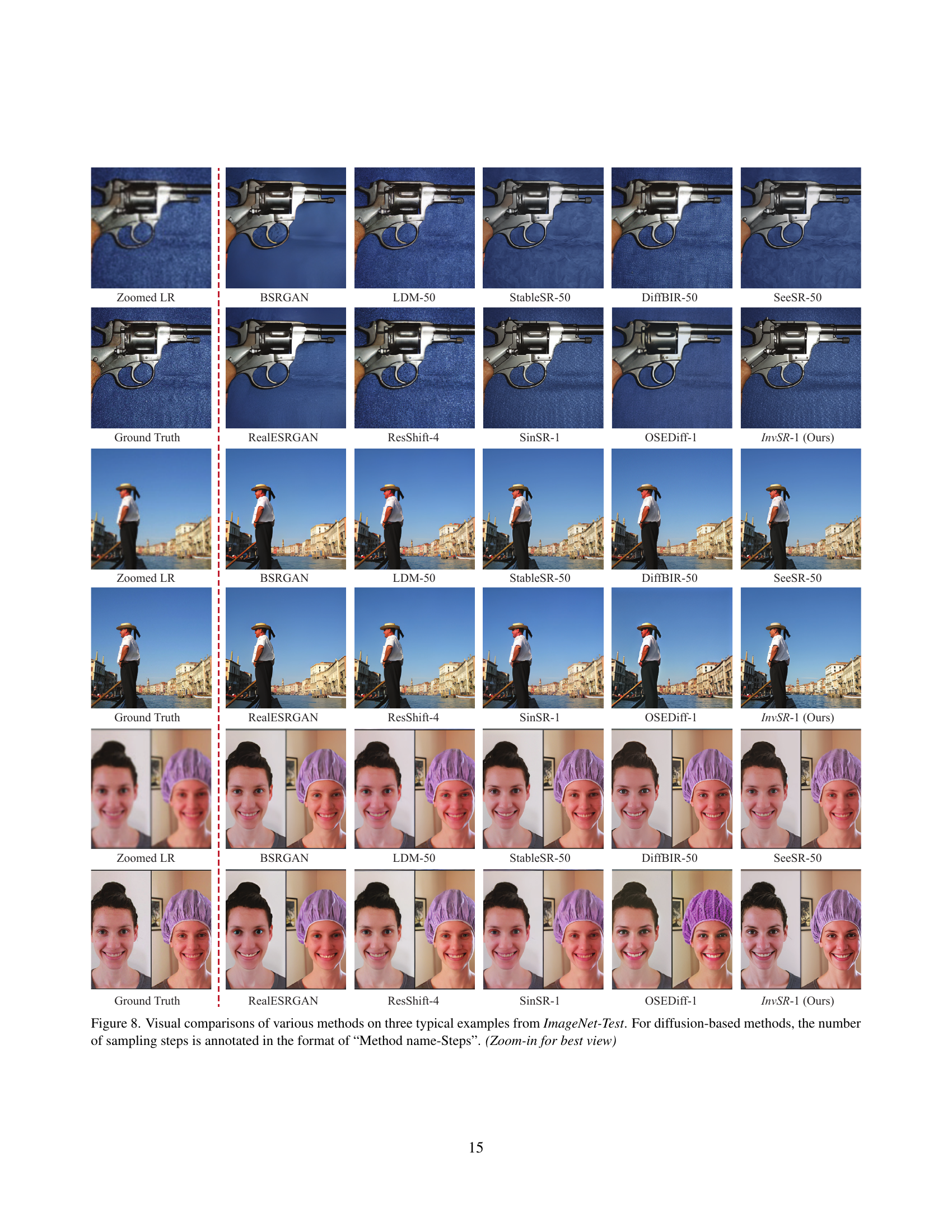
🔼 Figure 8 presents a qualitative comparison of different image super-resolution (SR) methods on three diverse examples sourced from the ImageNet-Test dataset. The figure showcases the results of various techniques, including both GAN-based and diffusion-based approaches. For the diffusion-based SR models, the number of sampling steps used during the SR process is explicitly indicated in the format of ‘Method Name-Steps’. This visual comparison allows for a direct assessment of the relative strengths and weaknesses of each method in terms of detail preservation, artifact reduction, and overall image quality. The caption suggests zooming in for a more detailed examination of the results.
read the caption
Figure 8: Visual comparisons of various methods on three typical examples from ImageNet-Test. For diffusion-based methods, the number of sampling steps is annotated in the format of “Method name-Steps”. (Zoom-in for best view)
More on tables
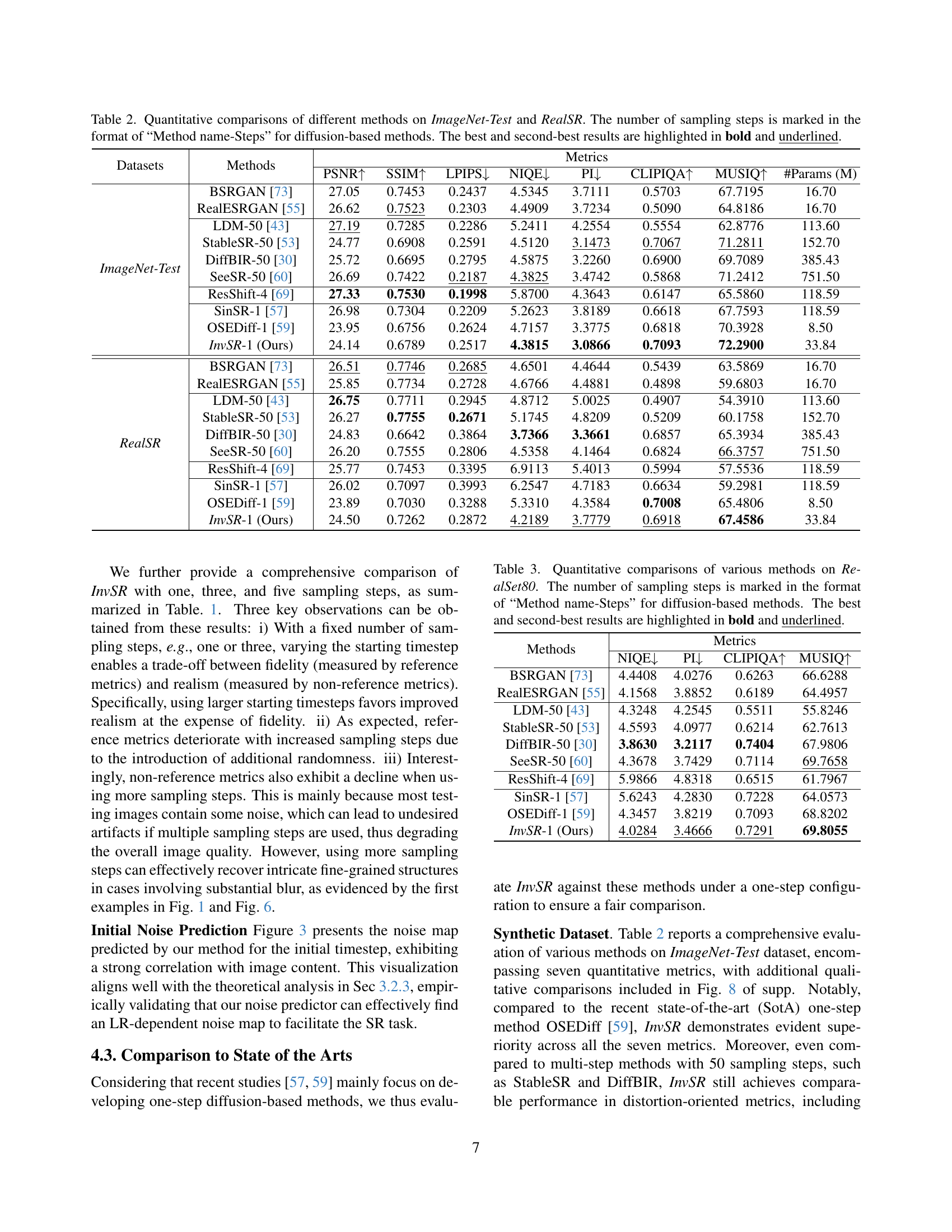
| Datasets | Methods | PSNR ↑ | SSIM ↑ | LPIPS ↓ | NIQE ↓ | PI ↓ | CLIPIQA ↑ | MUSIQ ↑ | #Params (M) | |
|---|---|---|---|---|---|---|---|---|---|---|
| ImageNet-Test | BSRGAN [73] | 27.05 | 0.7453 | 0.2437 | 4.5345 | 3.7111 | 0.5703 | 67.7195 | 16.70 | |
| RealESRGAN [55] | 26.62 | 0.7523 | 0.2303 | 4.4909 | 3.7234 | 0.5090 | 64.8186 | 16.70 | ||
| ImageNet-Test | LDM-50 [43] | 27.19 | 0.7285 | 0.2286 | 5.2411 | 4.2554 | 0.5554 | 62.8776 | 113.60 | |
| StableSR-50 [53] | 24.77 | 0.6908 | 0.2591 | 4.5120 | 3.1473 | 0.7067 | 71.2811 | 152.70 | ||
| DiffBIR-50 [30] | 25.72 | 0.6695 | 0.2795 | 4.5875 | 3.2260 | 0.6900 | 69.7089 | 385.43 | ||
| SeeSR-50 [60] | 26.69 | 0.7422 | 0.2187 | 4.3825 | 3.4742 | 0.5868 | 71.2412 | 751.50 | ||
| RealSR | BSRGAN [73] | 26.51 | 0.7746 | 0.2685 | 4.6501 | 4.4644 | 0.5439 | 63.5869 | 16.70 | |
| RealESRGAN [55] | 25.85 | 0.7734 | 0.2728 | 4.6766 | 4.4881 | 0.4898 | 59.6803 | 16.70 | ||
| LDM-50 [43] | 26.75 | 0.7711 | 0.2945 | 4.8712 | 5.0025 | 0.4907 | 54.3910 | 113.60 | ||
| StableSR-50 [53] | 26.27 | 0.7755 | 0.2671 | 5.1745 | 4.8209 | 0.5209 | 60.1758 | 152.70 | ||
| DiffBIR-50 [30] | 24.83 | 0.6642 | 0.3864 | 3.7366 | 3.3661 | 0.6857 | 65.3934 | 385.43 | ||
| SeeSR-50 [60] | 26.20 | 0.7555 | 0.2806 | 4.5358 | 4.1464 | 0.6824 | 66.3757 | 751.50 | ||
| ResShift-4 [69] | 25.77 | 0.7453 | 0.3395 | 6.9113 | 5.4013 | 0.5994 | 57.5536 | 118.59 | ||
| SinSR-1 [57] | 26.98 | 0.7304 | 0.2209 | 5.2623 | 3.8189 | 0.6618 | 67.7593 | 118.59 | ||
| OSEDiff-1 [59] | 23.95 | 0.6756 | 0.2624 | 4.7157 | 3.3775 | 0.6818 | 70.3928 | 8.50 | ||
| InvSR-1 (Ours) | 24.14 | 0.6789 | 0.2517 | 4.3815 | 3.0866 | 0.7093 | 72.2900 | 33.84 | ||
| InvSR-1 (Ours) | 24.50 | 0.7262 | 0.2872 | 4.2189 | 3.7779 | 0.6918 | 67.4586 | 33.84 |
🔼 Table 2 presents a quantitative comparison of several image super-resolution (SR) methods on two datasets: ImageNet-Test and RealSR. The table evaluates performance using a range of metrics, including PSNR, SSIM, LPIPS, NIQE, PI, CLIPIQA, and MUSIQ. For diffusion-based methods, the number of sampling steps used is indicated, allowing for a comparison of performance across various approaches with differing computational costs. The best and second-best results for each metric on each dataset are highlighted for easy identification.
read the caption
Table 2: Quantitative comparisons of different methods on ImageNet-Test and RealSR. The number of sampling steps is marked in the format of “Method name-Steps” for diffusion-based methods. The best and second-best results are highlighted in bold and underlined.
| Methods | NIQE ↓ | PI ↓ | CLIPIQA ↑ | MUSIQ ↑ |
|---|---|---|---|---|
| 5 | ||||
| BSRGAN [73] | 4.4408 | 4.0276 | 0.6263 | 66.6288 |
| RealESRGAN [55] | 4.1568 | 3.8852 | 0.6189 | 64.4957 |
| LDM-50 [43] | 4.3248 | 4.2545 | 0.5511 | 55.8246 |
| StableSR-50 [53] | 4.5593 | 4.0977 | 0.6214 | 62.7613 |
| DiffBIR-50 [30] | 3.8630 | 3.2117 | 0.7404 | 67.9806 |
| SeeSR-50 [60] | 4.3678 | 3.7429 | 0.7114 | 69.7658 |
| ResShift-4 [69] | 5.9866 | 4.8318 | 0.6515 | 61.7967 |
| SinSR-1 [57] | 5.6243 | 4.2830 | 0.7228 | 64.0573 |
| OSEDiff-1 [59] | 4.3457 | 3.8219 | 0.7093 | 68.8202 |
| InvSR-1 (Ours) | 4.0284 | 3.4666 | 0.7291 | 69.8055 |
🔼 Table 3 presents a quantitative comparison of different image super-resolution (SR) methods on the RealSet80 dataset. The table shows performance metrics for various methods, including both traditional GAN-based methods (BSRGAN, RealESRGAN) and diffusion-based methods (LDM, StableSR, DiffBIR, SeeSR, ResShift, SinSR, OSEDiff, and InvSR). For diffusion-based methods, the number of sampling steps used is explicitly stated in the method name (e.g., LDM-50 indicates 50 sampling steps). The metrics used to evaluate the SR performance include several no-reference image quality metrics (NIQE, PI, CLIPIQA, MUSIQ). The best and second-best performing methods for each metric are highlighted in bold and underlined for easy comparison. This table provides a quantitative assessment of the relative strengths and weaknesses of various SR approaches, specifically highlighting how the proposed InvSR method performs compared to other state-of-the-art techniques.
read the caption
Table 3: Quantitative comparisons of various methods on RealSet80. The number of sampling steps is marked in the format of “Method name-Steps” for diffusion-based methods. The best and second-best results are highlighted in bold and underlined.
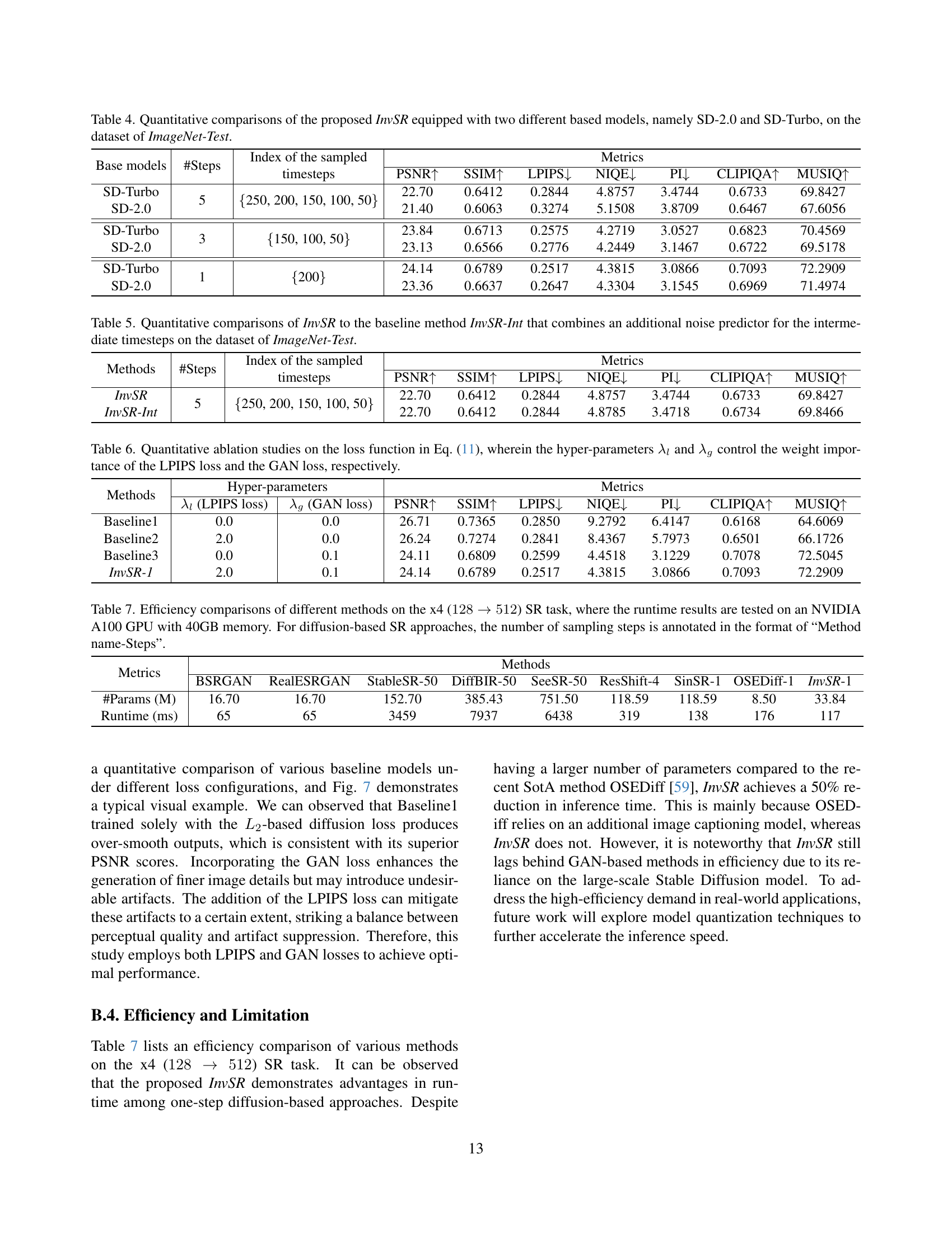
| Base models | #Steps | Index of the sampled timesteps | PSNR↑ | SSIM↑ | LPIPS↓ | NIQE↓ | PI↓ | CLIPIQA↑ | MUSIQ↑ |
|---|---|---|---|---|---|---|---|---|---|
| 10 | |||||||||
| SD-Turbo | 5 | {250, 200, 150, 100, 50} | 22.70 | 0.6412 | 0.2844 | 4.8757 | 3.4744 | 0.6733 | 69.8427 |
| SD-2.0 | 21.40 | 0.6063 | 0.3274 | 5.1508 | 3.8709 | 0.6467 | 67.6056 | ||
| SD-Turbo | 3 | {150, 100, 50} | 23.84 | 0.6713 | 0.2575 | 4.2719 | 3.0527 | 0.6823 | 70.4569 |
| SD-2.0 | 23.13 | 0.6566 | 0.2776 | 4.2449 | 3.1467 | 0.6722 | 69.5178 | ||
| SD-Turbo | 1 | {200} | 24.14 | 0.6789 | 0.2517 | 4.3815 | 3.0866 | 0.7093 | 72.2909 |
| SD-2.0 | 23.36 | 0.6637 | 0.2647 | 4.3304 | 3.1545 | 0.6969 | 71.4974 |
🔼 This table presents a quantitative comparison of the performance of the proposed InvSR model using two different pre-trained diffusion models as its base: Stable Diffusion 2.0 and Stable Diffusion Turbo. The comparison is done on the ImageNet-Test dataset and uses several metrics such as PSNR, SSIM, LPIPS, NIQE, PI, CLIPIQA, and MUSIQ to evaluate the image quality of super-resolution results. The results are shown for different numbers of sampling steps to demonstrate the effect of this parameter on the final output. This helps in understanding how the choice of base model and the number of sampling steps affect the performance of the InvSR model.
read the caption
Table 4: Quantitative comparisons of the proposed InvSR equipped with two different based models, namely SD-2.0 and SD-Turbo, on the dataset of ImageNet-Test.
| Methods | #Steps | Index of the sampled timesteps | PSNR ↑ | SSIM ↑ | LPIPS ↓ | NIQE ↓ | PI ↓ | CLIPIQA ↑ | MUSIQ ↑ |
|---|---|---|---|---|---|---|---|---|---|
| 10 | |||||||||
| InvSR | 5 | {250, 200, 150, 100, 50} | 22.70 | 0.6412 | 0.2844 | 4.8757 | 3.4744 | 0.6733 | 69.8427 |
| InvSR-Int | 22.70 | 0.6412 | 0.2844 | 4.8785 | 3.4718 | 0.6734 | 69.8466 | ||
🔼 This table presents a quantitative comparison of two methods on the ImageNet-Test dataset: InvSR and InvSR-Int. InvSR is the proposed method, while InvSR-Int is a modified version that incorporates an extra noise predictor for intermediate steps in the diffusion process. The comparison uses several metrics (PSNR, SSIM, LPIPS, NIQE, PI, CLIPIQA, and MUSIQ) to evaluate the performance of both methods, which helps assess the impact of adding the extra noise predictor for intermediate steps on the overall image quality.
read the caption
Table 5: Quantitative comparisons of InvSR to the baseline method InvSR-Int that combines an additional noise predictor for the intermediate timesteps on the dataset of ImageNet-Test.
| Methods | λl (LPIPS loss) | λg (GAN loss) | PSNR ↑ | SSIM ↑ | LPIPS ↓ | NIQE ↓ | PI ↓ | CLIPIQA ↑ | MUSIQ ↑ |
|---|---|---|---|---|---|---|---|---|---|
| 10 | 26.71 | 0.7365 | 0.2850 | 9.2792 | 6.4147 | 0.6168 | 64.6069 | ||
| Baseline1 | 0.0 | 0.0 | 26.71 | 0.7365 | 0.2850 | 9.2792 | 6.4147 | 0.6168 | 64.6069 |
| Baseline2 | 2.0 | 0.0 | 26.24 | 0.7274 | 0.2841 | 8.4367 | 5.7973 | 0.6501 | 66.1726 |
| Baseline3 | 0.0 | 0.1 | 24.11 | 0.6809 | 0.2599 | 4.4518 | 3.1229 | 0.7078 | 72.5045 |
| InvSR-1 | 2.0 | 0.1 | 24.14 | 0.6789 | 0.2517 | 4.3815 | 3.0866 | 0.7093 | 72.2909 |
🔼 This table presents an ablation study on the impact of different loss functions used in training the noise predictor model. It shows the results of using different combinations of the LPIPS (Learned Perceptual Image Patch Similarity) loss and the GAN (Generative Adversarial Network) loss, quantified by their respective hyperparameters λl (lambda_l) and λg (lambda_g). The study evaluates the effectiveness of each loss combination on several key metrics, such as PSNR, SSIM, LPIPS, NIQE, PI, CLIPIQA, and MUSIQ, to determine the optimal configuration for achieving high-quality image super-resolution.
read the caption
Table 6: Quantitative ablation studies on the loss function in Eq. (11), wherein the hyper-parameters λlsubscript𝜆𝑙\lambda_{l}italic_λ start_POSTSUBSCRIPT italic_l end_POSTSUBSCRIPT and λgsubscript𝜆𝑔\lambda_{g}italic_λ start_POSTSUBSCRIPT italic_g end_POSTSUBSCRIPT control the weight importance of the LPIPS loss and the GAN loss, respectively.
| Metrics | Methods | ||||||||
|---|---|---|---|---|---|---|---|---|---|
| 10 | |||||||||
| BSRGAN | RealESRGAN | StableSR-50 | DiffBIR-50 | SeeSR-50 | ResShift-4 | SinSR-1 | OSEDiff-1 | InvSR-1 | |
| #Params (M) | 16.70 | 16.70 | 152.70 | 385.43 | 751.50 | 118.59 | 118.59 | 8.50 | 33.84 |
| Runtime (ms) | 65 | 65 | 3459 | 7937 | 6438 | 319 | 138 | 176 | 117 |
🔼 Table 7 presents a comparison of the computational efficiency of various image super-resolution (SR) methods. The comparison focuses on the speed of the algorithms when performing a 4x upscaling task (increasing the resolution from 128x128 to 512x512 pixels). The runtime was measured using an NVIDIA A100 GPU with 40GB of memory. For methods that utilize diffusion models, the number of sampling steps employed is also specified. This table helps to illustrate the trade-off between model complexity (as indicated by the number of parameters), computational time, and the quality of super-resolution achieved.
read the caption
Table 7: Efficiency comparisons of different methods on the x4 (128→512→128512128\rightarrow 512128 → 512) SR task, where the runtime results are tested on an NVIDIA A100 GPU with 40GB memory. For diffusion-based SR approaches, the number of sampling steps is annotated in the format of “Method name-Steps”.
Full paper#
