↗ arXiv ↗ Hugging Face ↗ Papers with Code
TL;DR#
Current multimodal large language models (MLLMs) struggle with visual understanding because they primarily use natural language supervision during training. This reliance on text alone overlooks opportunities to directly optimize the model’s visual representation. This paper introduces OLA-VLM, a novel approach that tackles this issue.
OLA-VLM leverages auxiliary embedding distillation, incorporating knowledge from specialized visual encoders into the LLM’s hidden layers during pretraining. This process improves the model’s understanding of visual information without requiring extra visual inputs during inference, resulting in improved efficiency and performance. Experiments demonstrate OLA-VLM outperforms existing methods across several benchmark tasks, highlighting the effectiveness of embedding distillation in enhancing MLLMs’ visual reasoning capabilities.
Key Takeaways#
Why does it matter?#
This paper is important because it addresses a critical limitation in current multimodal large language models (MLLMs): their suboptimal visual understanding abilities due to relying solely on natural language supervision. By introducing a novel embedding distillation technique, OLA-VLM, the researchers significantly improve the visual perception capabilities of MLLMs, opening new avenues for research in enhancing the visual reasoning powers of these models. This work’s findings and methodology are highly relevant to current trends in MLLM development, offering a potential solution to a significant challenge. It could inspire further research into optimizing MLLM representations using knowledge distillation from various specialized models.
Visual Insights#
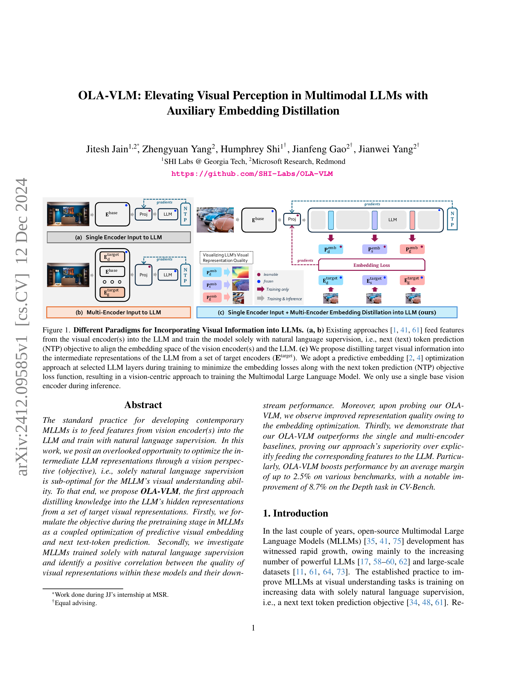
🔼 This figure illustrates three different methods for integrating visual information into large language models (LLMs). (a) and (b) show existing methods that feed visual features directly into the LLM, relying solely on natural language training. In contrast, (c) presents the proposed OLA-VLM approach, which distills visual information from multiple specialized encoders into the LLM’s intermediate layers during training. This allows for a more vision-centric training process, ultimately improving visual understanding without the need for multiple visual encoders during inference.
read the caption
Figure 1: Different Paradigms for Incorporating Visual Information into LLMs. (a, b) Existing approaches [41, 1, 61] feed features from the visual encoder(s) into the LLM and train the model solely with natural language supervision, i.e., next (text) token prediction (NTP) objective to align the embedding space of the vision encoder(s) and the LLM. (c) We propose distilling target visual information into the intermediate representations of the LLM from a set of target encoders (𝐄targetsuperscript𝐄target\mathbf{E}^{\text{target}}bold_E start_POSTSUPERSCRIPT target end_POSTSUPERSCRIPT). We adopt a predictive embedding [2, 4] optimization approach at selected LLM layers during training to minimize the embedding losses along with the next token prediction (NTP) objective loss function, resulting in a vision-centric approach to training the Multimodal Large Language Model. We only use a single base vision encoder during inference.
| Method | Encoder | Count2D | Depth3D | Relation2D | Distance3D | MMStar | RWQA | OK-VQA | Avg |
|---|---|---|---|---|---|---|---|---|---|
| Phi3-4k-mini | |||||||||
| LLaVA-1.5 | CLIP-ViT-L | 52.4 | 67.2 | 75.2 | 56.3 | 36.5 | 57.1 | 56.7 | 57.3 |
| OLA-VLM (ours) | CLIP-ViT-L | 52.4 | 68.7 | 76.0 | 56.7 | 36.0 | 58.0 | 56.4 | 57.7 |
| LLaVA-1.5 | CLIP-ConvNeXT-XXL | 51.8 | 70.8 | 74.0 | 55.3 | 36.4 | 58.0 | 55.9 | 57.4 |
| OLA-VLM (ours) | CLIP-ConvNeXT-XXL | 49.4 | 72.5 | 77.2 | 60.3 | 38.4 | 58.4 | 56.5 | 58.9 |
| Llama3-8b | |||||||||
| LLaVA-1.5 | CLIP-ViT-L | 50.4 | 73.3 | 64.9 | 48.7 | 38.8 | 57.8 | 56.9 | 55.1 |
| LLaVA-1.5 (feat concat.) | CLIP-ViT-L + 𝐄depth + 𝐄seg + 𝐄gen | 45.3 | 75.5 | 70.9 | 54.3 | 36.1 | 57.5 | 58.3 | 56.8 |
| LLaVA-1.5 (token concat.) | CLIP-ViT-L + 𝐄depth + 𝐄seg + 𝐄gen | 45.9 | 75.7 | 68.9 | 52.7 | 37.8 | 56.5 | 59.3 | 56.7 |
| OLA-VLM (ours) | CLIP-ViT-L | 51.3 | 74.2 | 69.4 | 54.3 | 39.5 | 57.9 | 56.6 | 57.6 |
| LLaVA-1.5 | CLIP-ConvNeXT-XXL | 54.1 | 62.8 | 69.5 | 49.8 | 37.4 | 57.5 | 56.3 | 55.3 |
| OLA-VLM (ours) | CLIP-ConvNeXT-XXL | 57.4 | 71.5 | 66.8 | 52.8 | 38.5 | 55.0 | 59.0 | 57.3 |
🔼 Table 1 compares the performance of OLA-VLM against single and multi-encoder baseline models on various vision and language benchmarks. It shows the performance across different combinations of base vision encoders (CLIP-ViT-L, CLIP-ConvNeXT-XXL) and decoder LLMs (LLaMA-3-8b). The results demonstrate that OLA-VLM consistently outperforms both single-encoder and multi-encoder baselines, achieving an average improvement of up to 2.5% over the single-encoder models and 0.9% over the multi-encoder models across the benchmarks. The best-performing models for each encoder/decoder combination are highlighted in bold.
read the caption
Table 1: Comparisons to Single and Multi-Encoder Baselines. We present results across different base encoders and decoder LLMs. Our OLA-VLM outperforms the single encoder and multi encoder LLaVA-1.5 [41] by up to 2.5% and 0.9% on average across various benchmarks, respectively. The best numbers are set in bold for every base-encoder and decoder LLM combination.
In-depth insights#
Visual Probe Analysis#
A visual probe analysis within a multimodal large language model (MLLM) research paper would likely involve probing the internal representations of the model to assess its understanding of visual information. This could be achieved by training probe networks on specific visual tasks, like object recognition or scene understanding, using the MLLM’s hidden layer activations as input. By analyzing the probe network’s performance, researchers can gain insights into how effectively the LLM processes and integrates visual data. Key aspects would include examining the quality of visual representations at different layers, identifying which layers contribute most to visual understanding, and observing how the quality of representations changes with different training methodologies or data augmentation techniques. Such an analysis is vital for diagnosing weaknesses and guiding improvements in the model’s visual perception capabilities. The results would provide valuable evidence for evaluating the efficacy of different architectural designs or training strategies, leading to the development of more robust and accurate MLLMs.
Embedding Distillation#
Embedding distillation, in the context of multimodal large language models (MLLMs), presents a novel approach to enhance visual understanding. Instead of directly feeding visual features into the LLM, this technique distills knowledge from pre-trained visual encoders into the intermediate layers of the LLM. This indirect method allows the model to learn better visual representations without explicitly increasing computational cost or altering the basic architecture, as might happen when adding more visual encoders. The core idea is to leverage predictive embedding losses, comparing the LLM’s representations with those from the visual encoders. By minimizing these losses during pre-training, the LLM learns to capture crucial visual information, thus improving its performance on downstream visual reasoning tasks. The effectiveness of this approach is demonstrated by improved downstream task accuracy and improved representation quality as measured by probing experiments. Key advantages include enhanced efficiency and a focus on vision-centric optimization within the LLM’s internal representations, unlike traditional methods that largely rely on natural language supervision alone. This is a significant step towards creating more robust and effective MLLMs capable of deeper visual understanding.
OLA-VLM’s Superiority#
The paper demonstrates OLA-VLM’s superiority over existing multimodal LLMs through a series of experiments. OLA-VLM’s key innovation lies in its novel embedding distillation technique, which injects visual knowledge from specialized target encoders (trained on tasks like image segmentation and depth estimation) into the LLM’s internal representations during pre-training. This contrasts with prior methods that solely rely on natural language supervision, showcasing a more holistic and efficient approach to visual understanding. Probing experiments reveal that OLA-VLM cultivates significantly better quality visual representations within the LLM, leading to improved downstream performance on benchmarks like CV-Bench. The results show consistent performance gains across various tasks and models, with particularly notable improvements in depth estimation. The effectiveness of the distillation strategy is further supported by ablations, demonstrating the optimal combination of target encoders, loss functions, and training strategies. OLA-VLM successfully balances efficiency and effectiveness, requiring only a single vision encoder during inference while outperforming both single and multi-encoder baselines.
Ablation Studies#
Ablation studies systematically remove components of a model to assess their individual contributions. In the context of this research paper, this would involve a series of experiments where elements of the OLA-VLM architecture are selectively removed or altered (e.g., removing the embedding loss, changing the number of special tokens, or varying the layers for embedding losses). The results would highlight the importance of each component on the overall model performance, revealing whether the proposed embedding distillation technique and other architectural choices are indeed crucial for the improvements observed. Analyzing these ablation studies will reveal which aspects are essential for OLA-VLM’s success and which parts may be redundant or even detrimental. A careful analysis will confirm the efficacy of the proposed method, providing strong evidence supporting its contributions to the state-of-the-art. The results may also suggest areas for future improvements, for instance, finding optimal configurations or identifying less crucial elements to improve efficiency and reduce model complexity.
Future Research#
The authors suggest several promising avenues for future research. Expanding the range of teacher encoders beyond the three used (depth, segmentation, generation) is crucial. Including models like SigLIP and InternViT could significantly improve the model’s general reasoning capabilities. Incorporating additional teacher encoders focusing on lower-level visual information (motion, for example) and training on video data would enhance spatial and temporal reasoning. The predictive embedding optimization technique could be extended to other modalities beyond vision. Investigating how the distillation of one type of information influences others warrants exploration. Furthermore, a more thorough investigation into the optimal placement of embedding losses within the LLM architecture is needed. Finally, experimenting with different embedding loss functions and optimization strategies could potentially lead to further improvements in performance and efficiency.
More visual insights#
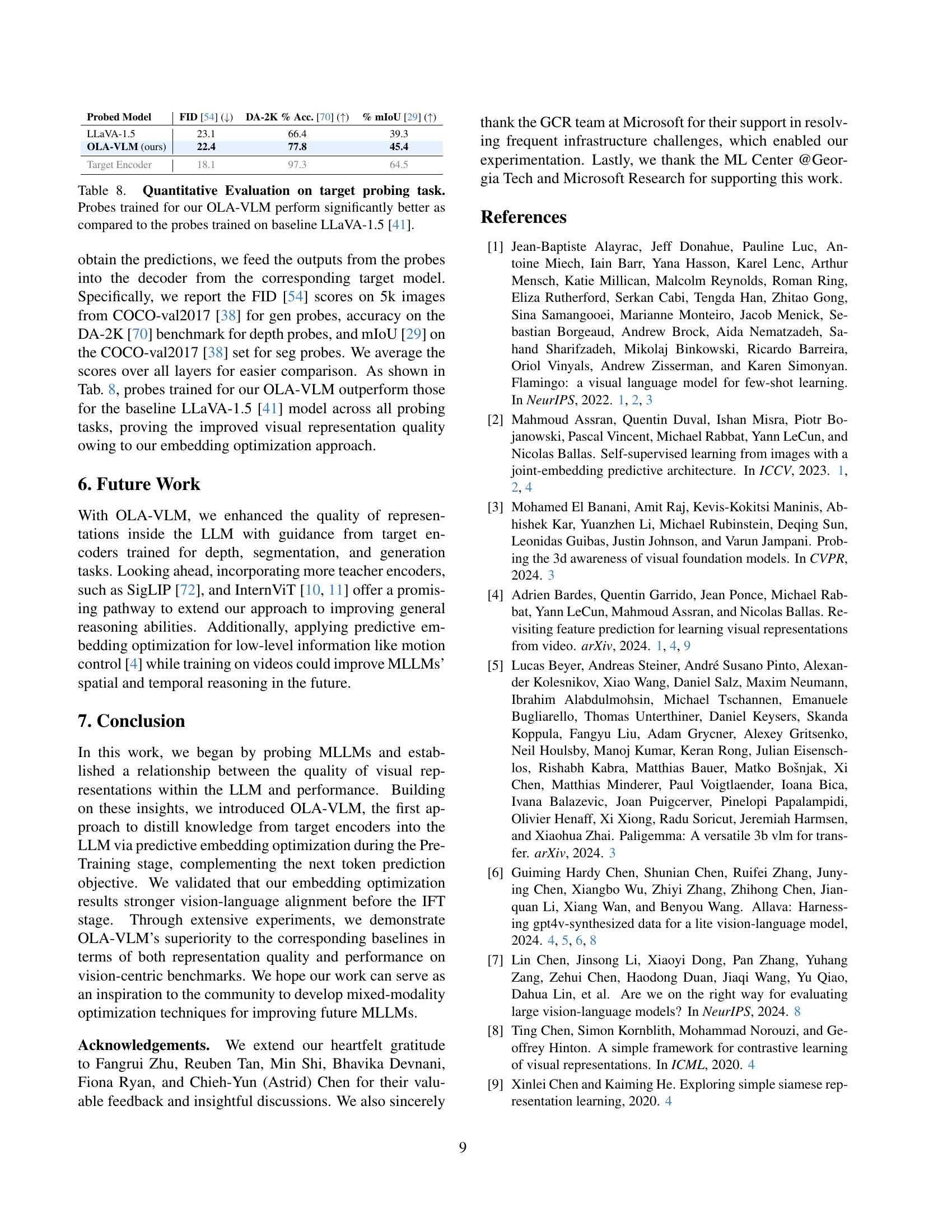
More on figures

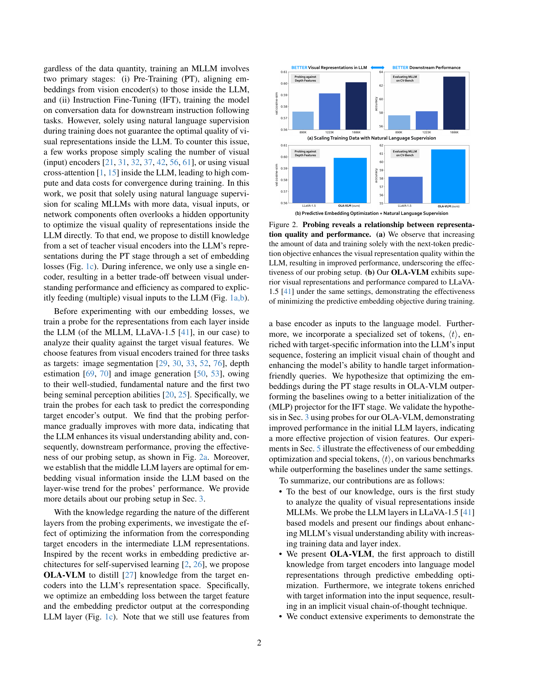
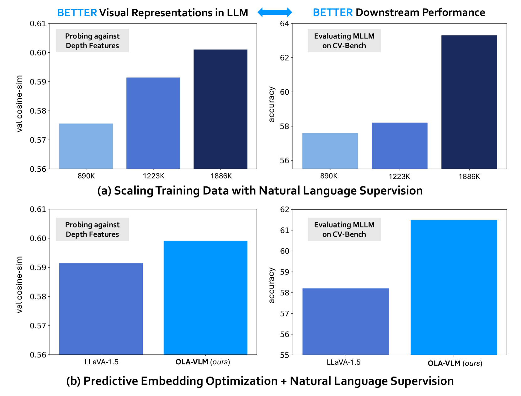
🔼 Figure 2 demonstrates the correlation between the quality of visual representations within a large language model (LLM) and its downstream performance. Panel (a) shows that training an LLM with solely natural language supervision (next-token prediction) leads to improved visual representation quality as the training data size increases, which in turn boosts performance. This validates the probing methodology used in the study. Panel (b) compares the proposed OLA-VLM with the LLaVA-1.5 baseline. OLA-VLM, incorporating predictive embedding optimization, shows significantly superior visual representation quality and performance, highlighting the effectiveness of the proposed method.
read the caption
Figure 2: Probing reveals a relationship between representation quality and performance. (a) We observe that increasing the amount of data and training solely with the next-token prediction objective enhances the visual representation quality within the LLM, resulting in improved performance, underscoring the effectiveness of our probing setup. (b) Our OLA-VLM exhibits superior visual representations and performance compared to LLaVA-1.5 [41] under the same settings, demonstrating the effectiveness of minimizing the predictive embedding objective during training.

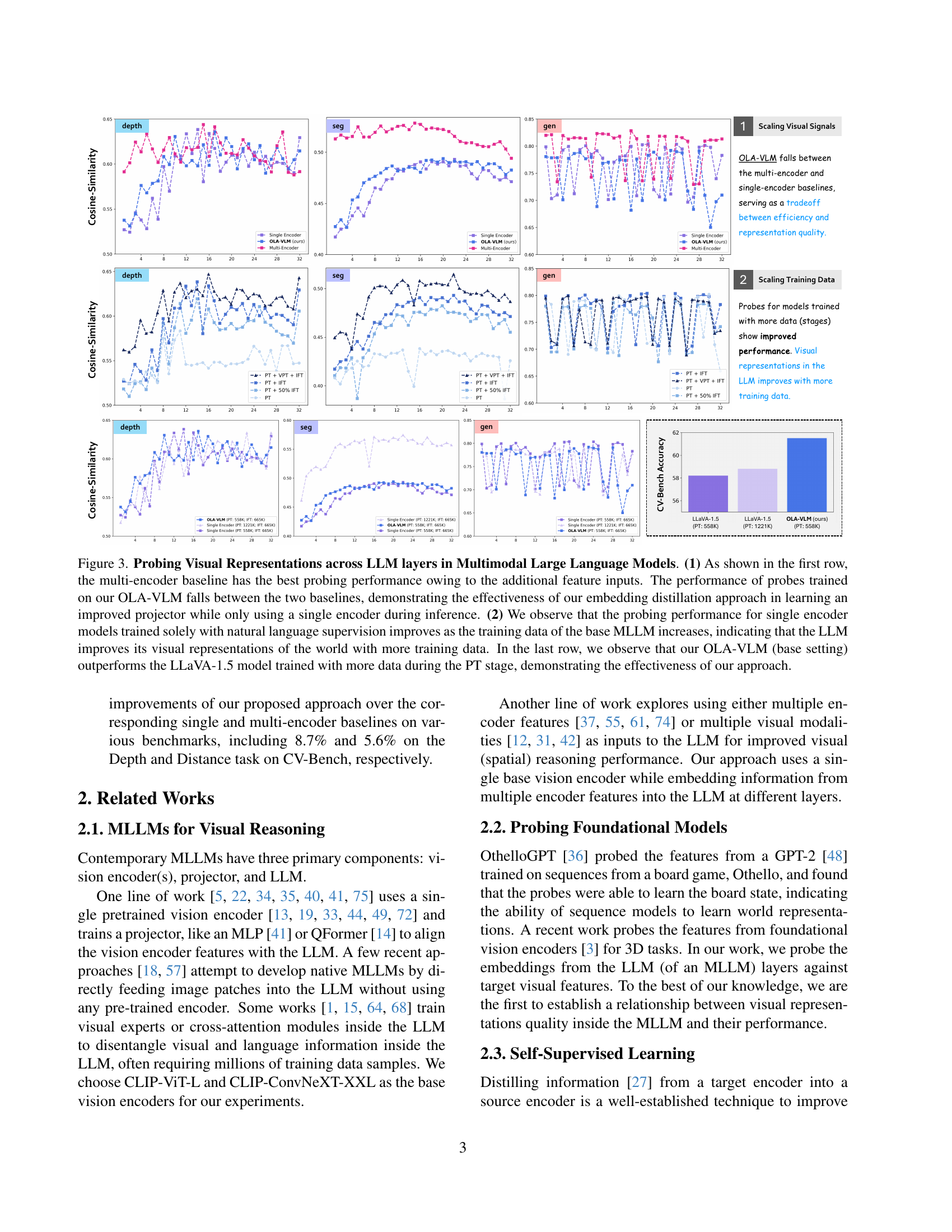
🔼 Figure 3 presents a comprehensive analysis of visual representation quality within different Multimodal Large Language Models (MLLMs) across various layers. The top row contrasts three different MLLM approaches: a single-encoder model, a multi-encoder model, and the authors’ proposed OLA-VLM model. It shows that the multi-encoder model achieves the best probing performance due to its access to more visual features. OLA-VLM, while using only a single encoder at inference time, demonstrates performance that falls between the single- and multi-encoder baselines, signifying the effectiveness of its knowledge distillation method for improving the projector’s ability to handle visual inputs. The middle row demonstrates how the probing performance of a single encoder model improves solely based on the amount of natural language training data used, highlighting the model’s ability to learn better visual representations with more data. Finally, the bottom row compares the base OLA-VLM against a LLaVA-1.5 model trained on a larger dataset, revealing that OLA-VLM still achieves better results, underscoring its ability to leverage a more efficient training approach.
read the caption
Figure 3: Probing Visual Representations across LLM layers in Multimodal Large Language Models. (1) As shown in the first row, the multi-encoder baseline has the best probing performance owing to the additional feature inputs. The performance of probes trained on our OLA-VLM falls between the two baselines, demonstrating the effectiveness of our embedding distillation approach in learning an improved projector while only using a single encoder during inference. (2) We observe that the probing performance for single encoder models trained solely with natural language supervision improves as the training data of the base MLLM increases, indicating that the LLM improves its visual representations of the world with more training data. In the last row, we observe that our OLA-VLM (base setting) outperforms the LLaVA-1.5 model trained with more data during the PT stage, demonstrating the effectiveness of our approach.

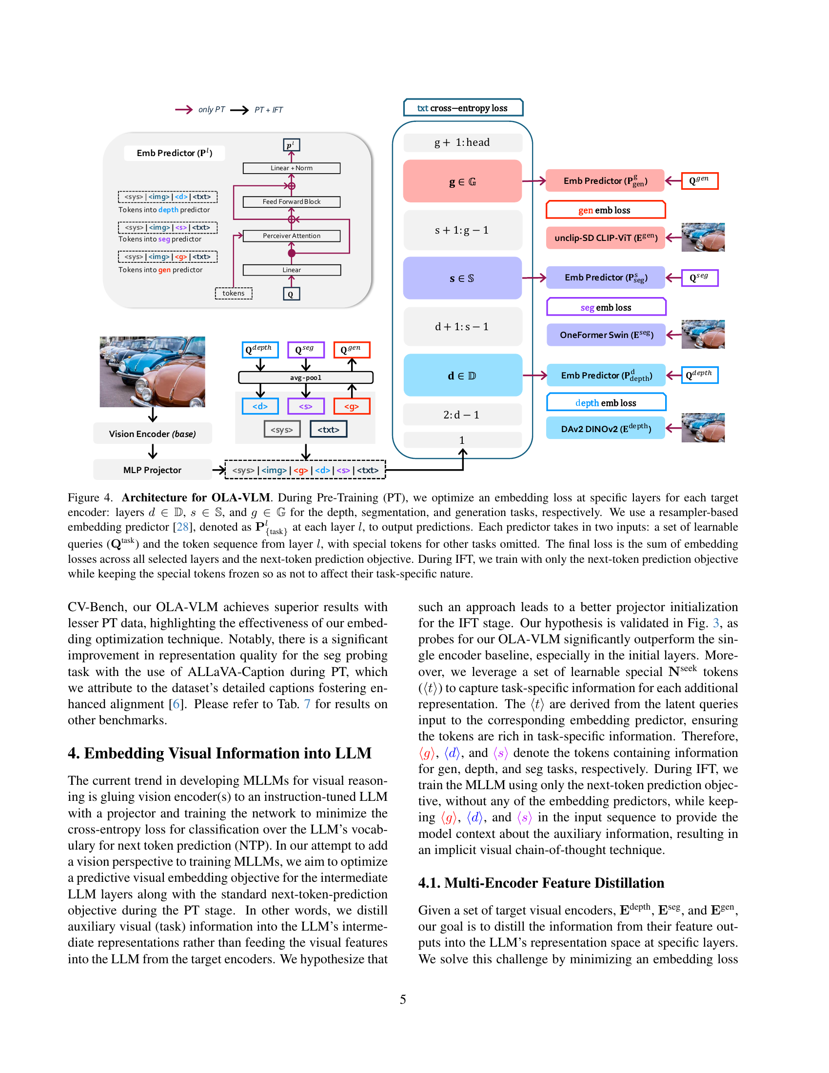
🔼 This figure illustrates the architecture of OLA-VLM, a multimodal large language model that incorporates visual information from multiple sources. During pre-training (PT), the model optimizes embedding losses at specific layers for each task (depth, segmentation, generation). These losses compare the model’s output to target encodings from specialized visual encoders, using a resampler-based embedding predictor. The predictor receives learnable queries and the model’s token sequence as input. The total loss combines these embedding losses with the standard next-token prediction loss. During instruction fine-tuning (IFT), only the next-token prediction loss is used, while task-specific special tokens are kept frozen to maintain their individual nature. This method aims to improve the model’s visual understanding by embedding task-specific information at various layers during pre-training, rather than solely relying on the natural language supervision.
read the caption
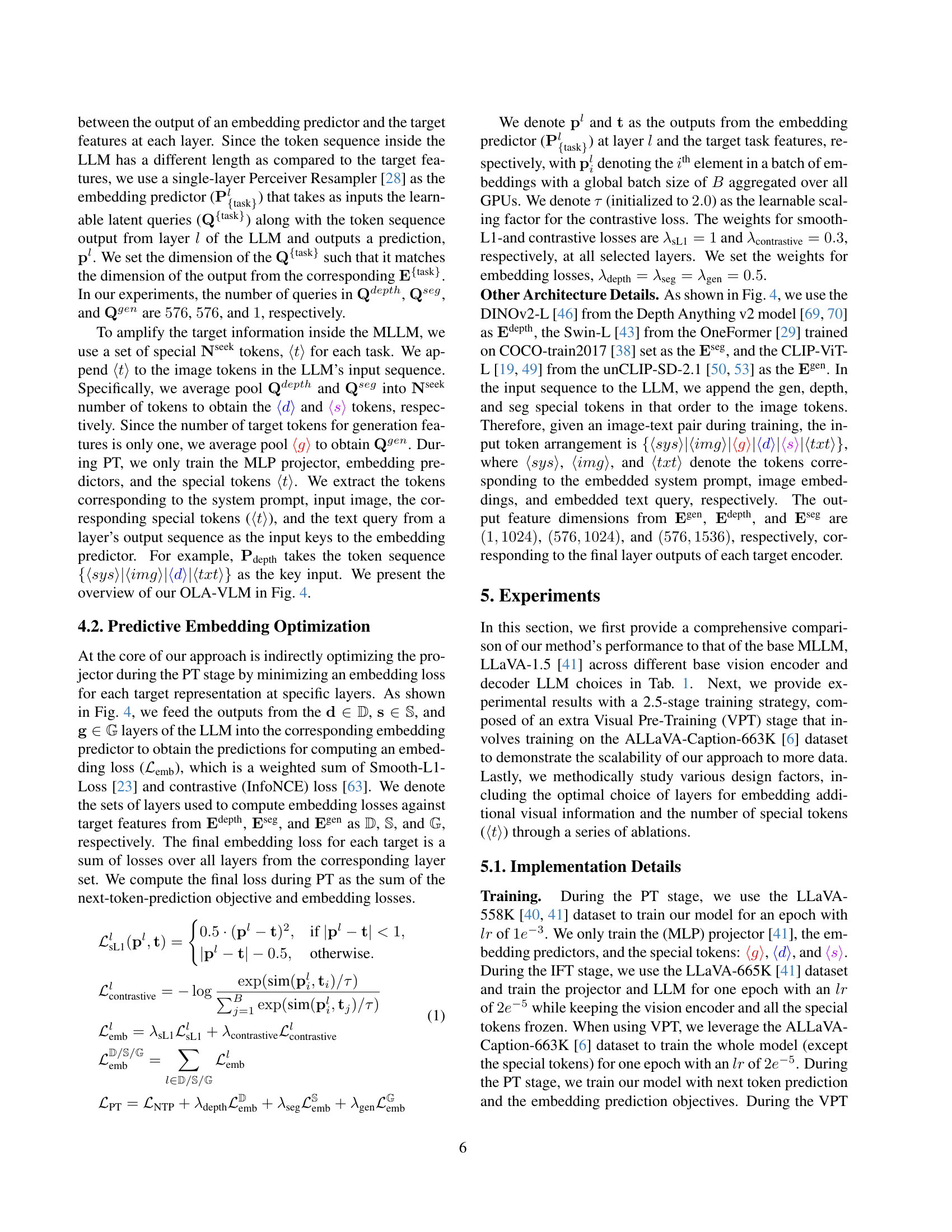
Figure 4: Architecture for OLA-VLM. During Pre-Training (PT), we optimize an embedding loss at specific layers for each target encoder: layers d∈𝔻𝑑𝔻d\in\mathbb{D}italic_d ∈ blackboard_D, s∈𝕊𝑠𝕊s\in\mathbb{S}italic_s ∈ blackboard_S, and g∈𝔾𝑔𝔾g\in\mathbb{G}italic_g ∈ blackboard_G for the depth, segmentation, and generation tasks, respectively. We use a resampler-based embedding predictor [28], denoted as 𝐏{task}lsubscriptsuperscript𝐏𝑙task\mathbf{P}^{l}_{\{\text{task}\}}bold_P start_POSTSUPERSCRIPT italic_l end_POSTSUPERSCRIPT start_POSTSUBSCRIPT { task } end_POSTSUBSCRIPT at each layer l𝑙litalic_l, to output predictions. Each predictor takes in two inputs: a set of learnable queries (𝐐tasksuperscript𝐐task\mathbf{Q}^{{\text{task}}}bold_Q start_POSTSUPERSCRIPT task end_POSTSUPERSCRIPT) and the token sequence from layer l𝑙litalic_l, with special tokens for other tasks omitted. The final loss is the sum of embedding losses across all selected layers and the next-token prediction objective. During IFT, we train with only the next-token prediction objective while keeping the special tokens frozen so as not to affect their task-specific nature.

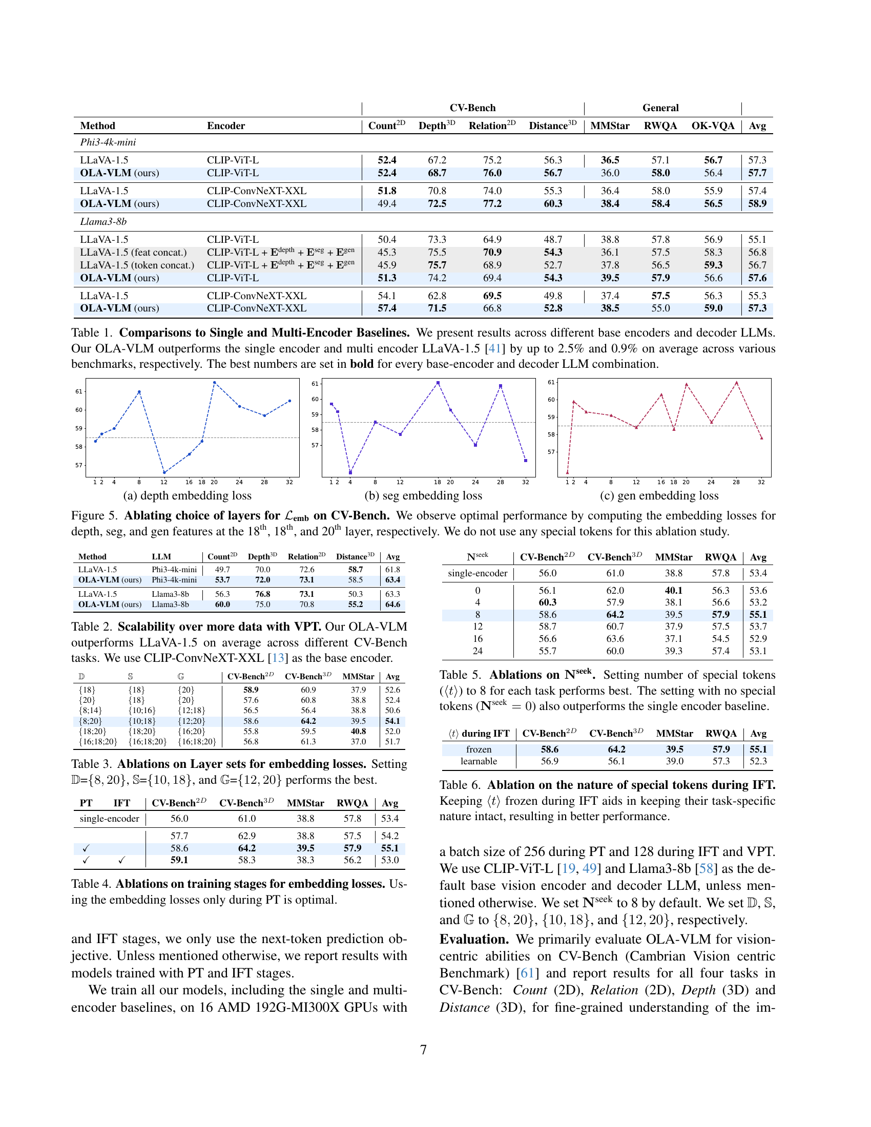
🔼 This figure shows the ablation study on the choice of layers for computing the depth embedding loss in the OLA-VLM model. The x-axis represents different layers in the LLM, and the y-axis represents the cosine similarity between the probe’s prediction and the ground truth depth features. The plot shows that the optimal layer for computing the embedding loss is around layer 18, indicating the optimal layer to inject depth information from the teacher model into the LLM.
read the caption
(a) depth embedding loss

🔼 This figure shows the ablation study on the choice of layers for computing the segmentation embedding loss in the OLA-VLM model. The x-axis represents the layer number in the LLM, and the y-axis represents the cosine similarity between the probe’s output and the target segmentation features. The plot illustrates how different choices of layers for computing the embedding loss impact the quality of learned visual representations. The results indicate that choosing optimal layers for the loss calculation significantly enhances the performance of the model.
read the caption
(b) seg embedding loss

🔼 This figure shows the ablation study on the choice of layers for computing the generation embedding loss. It displays the performance on the CV-Bench benchmark for different layer selections, revealing the optimal layer choice for minimizing the generation embedding loss and achieving better performance.
read the caption
(c) gen embedding loss

🔼 This figure displays ablation studies on the choice of layers for calculating embedding loss (ℒemb) in the OLA-VLM model. The experiment was conducted using the CV-Bench benchmark. The x-axis represents the layer number of the Large Language Model (LLM) and the y-axis shows the cosine similarity. Three different tasks (depth, segmentation, generation) are considered, each represented by a different colored line. The results indicate that calculating embedding losses at the 18th layer for depth and segmentation tasks, and the 20th layer for the generation task yields the optimal performance. Notably, this experiment was performed without using any special tokens.
read the caption
Figure 5: Ablating choice of layers for ℒembsubscriptℒemb\mathcal{L}_{\text{emb}}caligraphic_L start_POSTSUBSCRIPT emb end_POSTSUBSCRIPT on CV-Bench. We observe optimal performance by computing the embedding losses for depth, seg, and gen features at the 18thth{}^{\text{th}}start_FLOATSUPERSCRIPT th end_FLOATSUPERSCRIPT, 18thth{}^{\text{th}}start_FLOATSUPERSCRIPT th end_FLOATSUPERSCRIPT, and 20thth{}^{\text{th}}start_FLOATSUPERSCRIPT th end_FLOATSUPERSCRIPT layer, respectively. We do not use any special tokens for this ablation study.

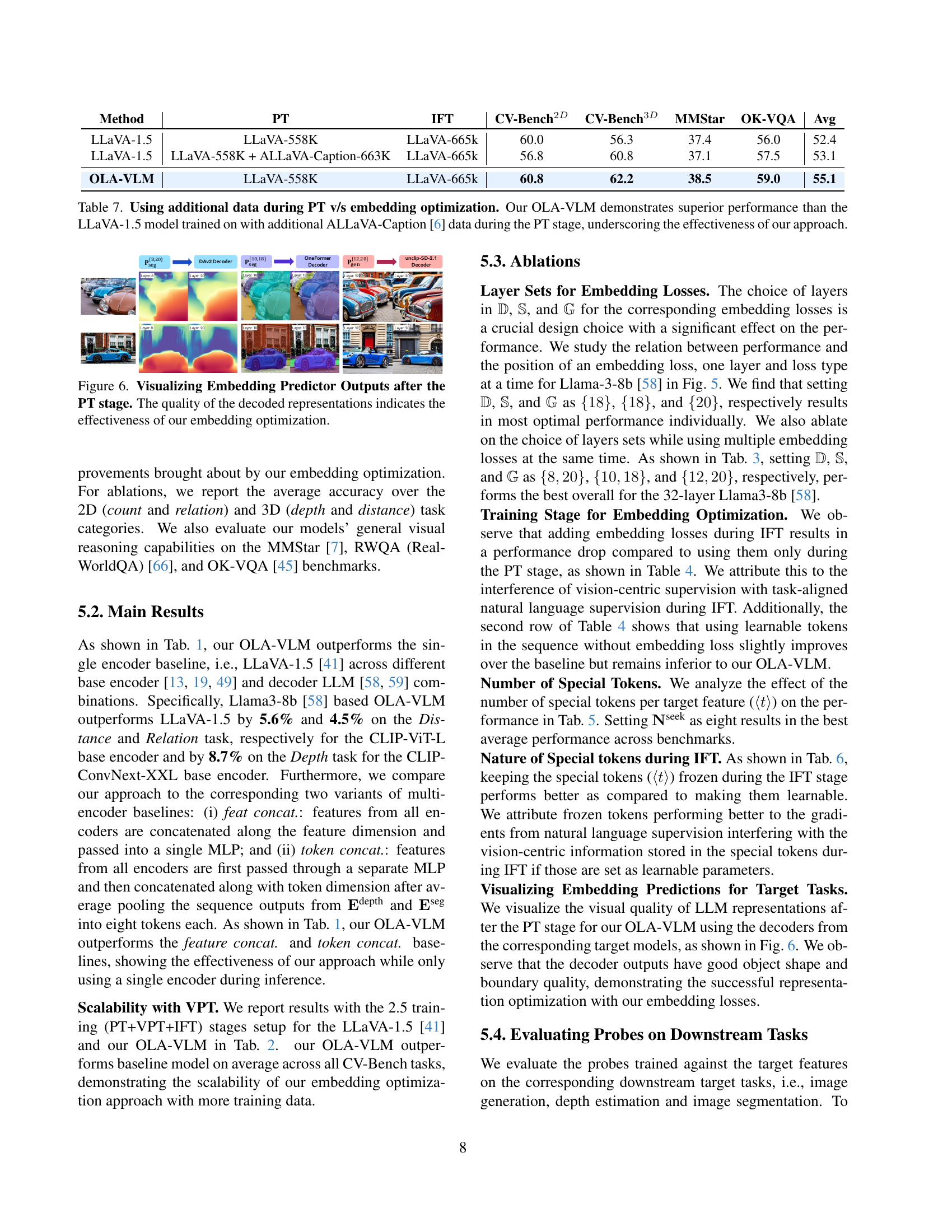
🔼 This figure visualizes the output of the embedding predictor models after the pre-training (PT) stage. Specifically, it shows the results of decoding the embedding predictor’s output using decoders from the target tasks (depth, segmentation, and generation). The visual quality of these decoded representations serves as a qualitative measure of the effectiveness of the proposed embedding optimization technique within OLA-VLM. The comparison of the results across different layers of the model offers insights into the layer-wise impact of the optimization strategy. High-quality decoded images suggest successful embedding optimization.
read the caption
Figure 6: Visualizing Embedding Predictor Outputs after the PT stage. The quality of the decoded representations indicates the effectiveness of our embedding optimization.
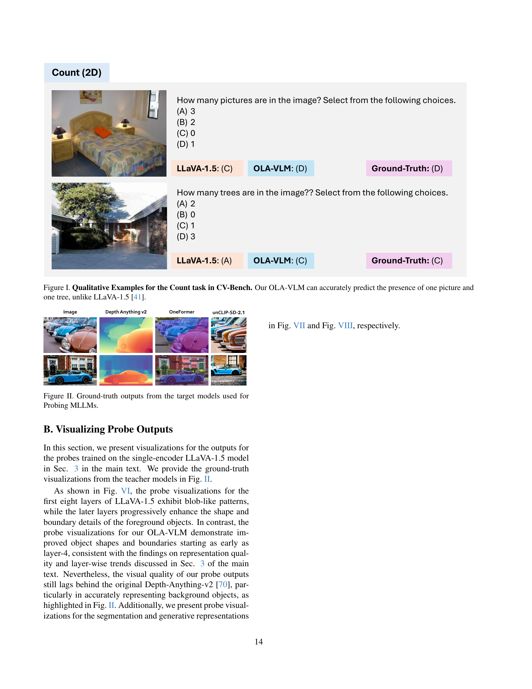
🔼 This figure presents two examples illustrating the performance of OLA-VLM and LLaVA-1.5 on the ‘Count’ task within the CV-Bench benchmark. The ‘Count’ task assesses the model’s ability to accurately count objects within an image. Each example shows an image alongside multiple-choice questions about the number of certain objects (e.g., pictures or trees). The ground truth answers are provided, demonstrating that OLA-VLM correctly identifies the number of pictures and trees in both example images, while LLaVA-1.5 makes incorrect predictions in both cases. This highlights OLA-VLM’s improved visual understanding and object counting capabilities.
read the caption
Figure I: Qualitative Examples for the Count task in CV-Bench. Our OLA-VLM can accurately predict the presence of one picture and one tree, unlike LLaVA-1.5 [41].

🔼 This figure displays the ground truth outputs generated by three different target models used in the probing experiments of the paper. These models represent different visual tasks: image segmentation, depth estimation, and image generation. Each model’s output provides a visual benchmark against which the LLM’s internal visual representations are compared to assess the quality of the LLM’s visual understanding. The figure is crucial for evaluating how effectively the OLA-VLM approach improves the LLM’s ability to capture and represent visual information, and offers a visual interpretation of the probing results.
read the caption
Figure II: Ground-truth outputs from the target models used for Probing MLLMs.

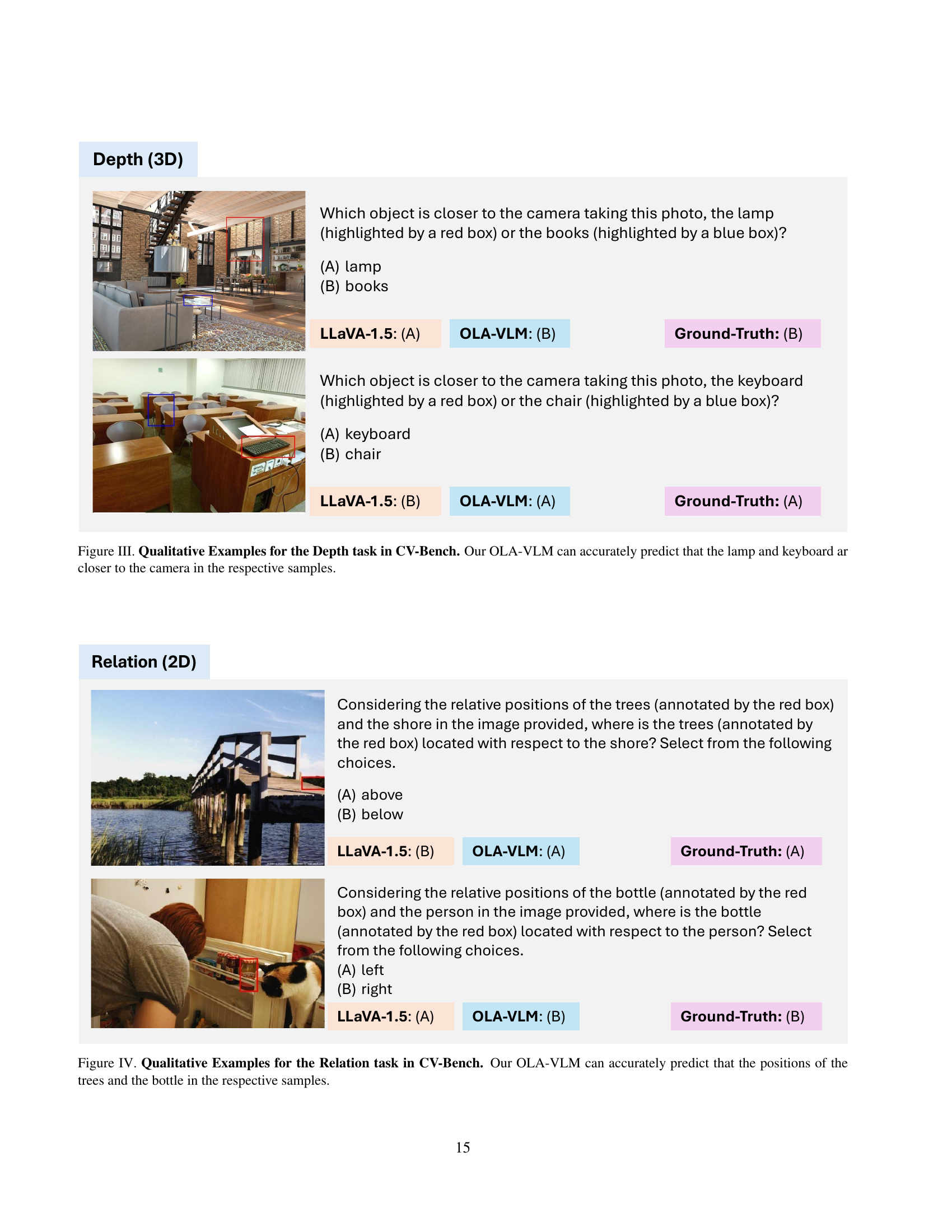
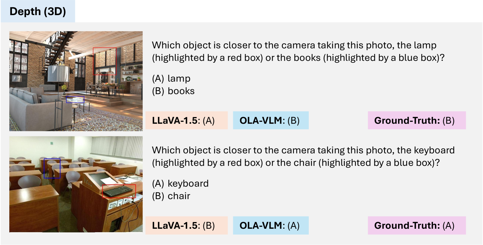
🔼 This figure showcases qualitative examples from the Depth task within the CV-Bench benchmark. It directly compares the performance of the OLA-VLM model against the LLaVA-1.5 baseline. Each example presents an image with two objects, one closer to the camera than the other. The caption highlights that OLA-VLM correctly identifies the closer object (lamp and keyboard) in both examples, while LLaVA-1.5 makes incorrect predictions.
read the caption
Figure III: Qualitative Examples for the Depth task in CV-Bench. Our OLA-VLM can accurately predict that the lamp and keyboard ar closer to the camera in the respective samples.

🔼 Figure IV showcases examples from the CV-Bench dataset’s Relation task, illustrating how OLA-VLM and LLaVA-1.5 models predict the spatial relationship between objects. The figure highlights OLA-VLM’s improved accuracy in determining the relative positions of objects (e.g., above/below, left/right) compared to the LLaVA-1.5 model.
read the caption
Figure IV: Qualitative Examples for the Relation task in CV-Bench. Our OLA-VLM can accurately predict that the positions of the trees and the bottle in the respective samples.

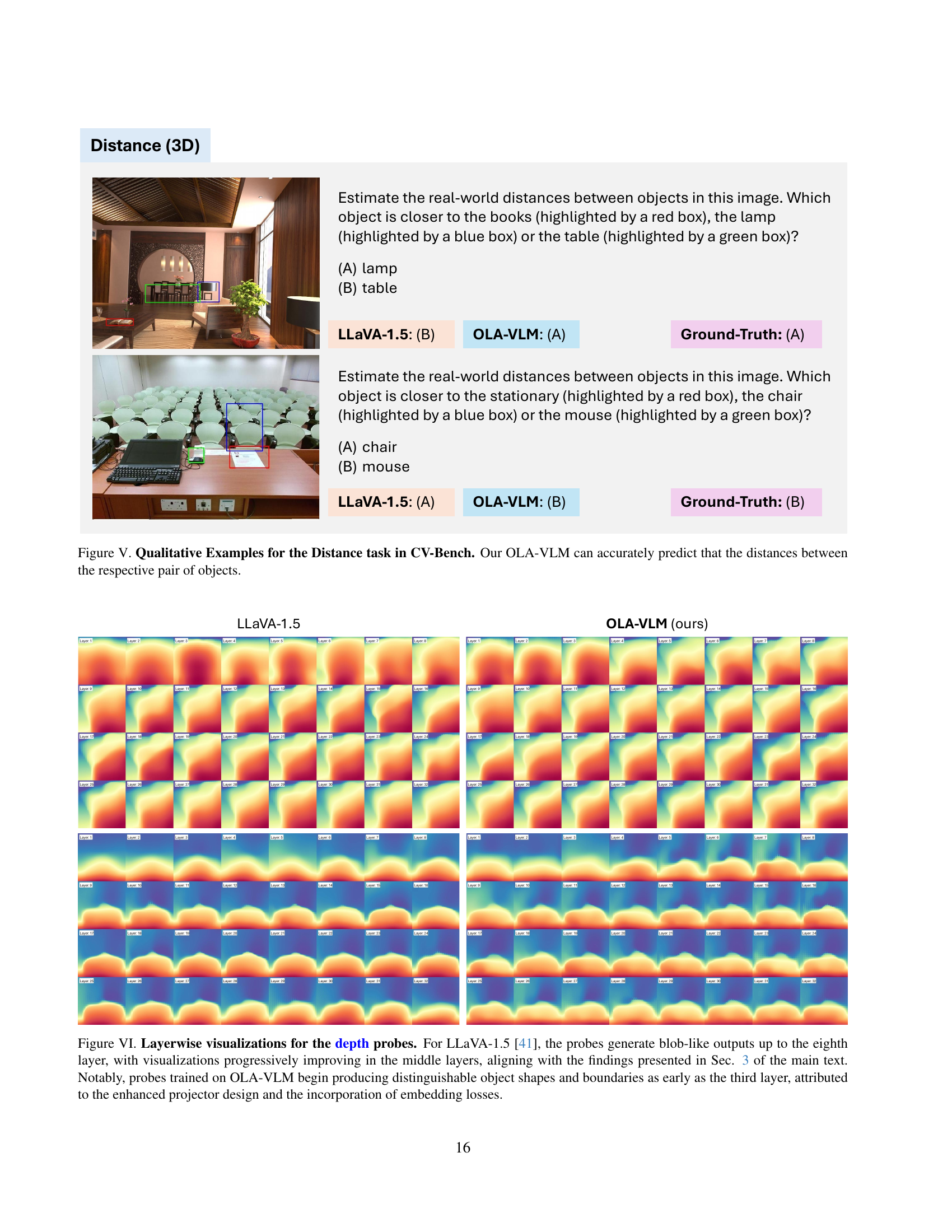
🔼 Figure V shows examples from the CV-Bench dataset’s Distance task, which evaluates the model’s ability to estimate real-world distances between objects in an image. Each example presents a scene with three objects, and the task is to identify which object is closest to a reference object. The figure highlights how OLA-VLM more accurately predicts the correct distances compared to the LLaVA-1.5 baseline. This demonstrates OLA-VLM’s improved performance in understanding and representing spatial relationships between objects.
read the caption
Figure V: Qualitative Examples for the Distance task in CV-Bench. Our OLA-VLM can accurately predict that the distances between the respective pair of objects.
🔼 This figure displays layer-wise visualizations of depth probe outputs for both LLaVA-1.5 and OLA-VLM. LLaVA-1.5 shows blob-like outputs for the first eight layers, gradually improving in the middle layers. In contrast, OLA-VLM produces distinguishable object shapes and boundaries from as early as the third layer, demonstrating the effectiveness of its enhanced projector and embedding loss techniques.
read the caption
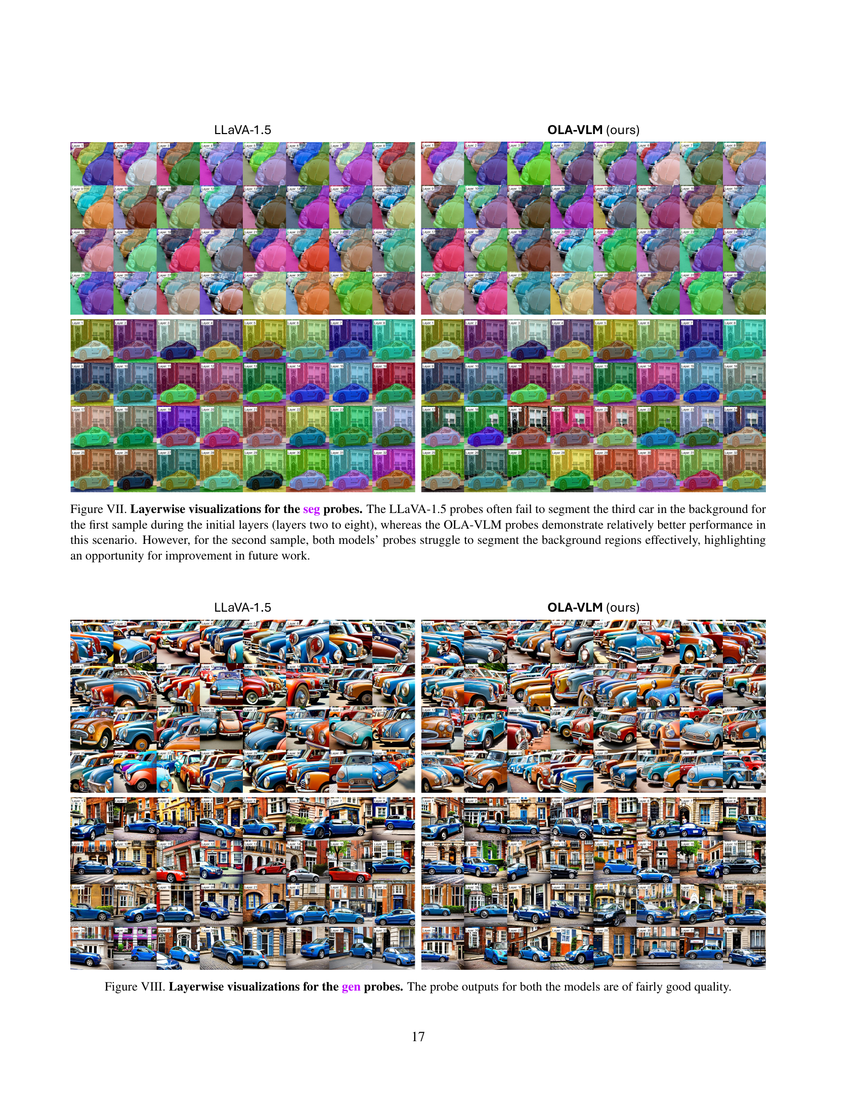
Figure VI: Layerwise visualizations for the depth probes. For LLaVA-1.5 [41], the probes generate blob-like outputs up to the eighth layer, with visualizations progressively improving in the middle layers, aligning with the findings presented in Sec. 3 of the main text. Notably, probes trained on OLA-VLM begin producing distinguishable object shapes and boundaries as early as the third layer, attributed to the enhanced projector design and the incorporation of embedding losses.
More on tables
| Method | LLM | Count2D | Depth3D | Relation2D | Distance3D | Avg |
|---|---|---|---|---|---|---|
| LLaVA-1.5 | Phi3-4k-mini | 49.7 | 70.0 | 72.6 | 58.7 | 61.8 |
| OLA-VLM (ours) | Phi3-4k-mini | 53.7 | 72.0 | 73.1 | 58.5 | 63.4 |
| LLaVA-1.5 | Llama3-8b | 56.3 | 76.8 | 73.1 | 50.3 | 63.3 |
| OLA-VLM (ours) | Llama3-8b | 60.0 | 75.0 | 70.8 | 55.2 | 64.6 |
🔼 Table 2 demonstrates the impact of additional visual data on the performance of OLA-VLM and LLaVA-1.5. Both models underwent pre-training (PT) and instruction fine-tuning (IFT) but OLA-VLM also included an additional visual pre-training (VPT) stage using the ALLaVA-Caption dataset. The table compares the performance of both models on various subtasks within the CV-Bench benchmark using CLIP-ConvNeXT-XXL as the base vision encoder. The results show that OLA-VLM consistently outperforms LLaVA-1.5 across all tasks, suggesting that the embedding distillation technique employed in OLA-VLM is particularly effective when combined with larger visual datasets.
read the caption
Table 2: Scalability over more data with VPT. Our OLA-VLM outperforms LLaVA-1.5 on average across different CV-Bench tasks. We use CLIP-ConvNeXT-XXL [13] as the base encoder.
| 𝔻 | 𝕊 | 𝔾 | CV-Bench2D | CV-Bench3D | MMStar | Avg |
|---|---|---|---|---|---|---|
| {18} | {18} | {20} | 58.9 | 60.9 | 37.9 | 52.6 |
| {20} | {18} | {20} | 57.6 | 60.8 | 38.8 | 52.4 |
| {8;14} | {10;16} | {12;18} | 56.5 | 56.4 | 38.8 | 50.6 |
| {8;20} | {10;18} | {12;20} | 58.6 | 64.2 | 39.5 | 54.1 |
| {18;20} | {18;20} | {16;20} | 55.8 | 59.5 | 40.8 | 52.0 |
| {16;18;20} | {16;18;20} | {16;18;20} | 56.8 | 61.3 | 37.0 | 51.7 |
🔼 This table presents ablation studies on different layer sets used for computing embedding losses in the OLA-VLM model. The goal is to determine the optimal layers within the Language Model (LLM) to incorporate visual information from target encoders. The results show the performance on various metrics across different sets of layers, with the combination of layers 8 and 20 for depth features (D), layers 10 and 18 for segmentation features (S), and layers 12 and 20 for generation features (G) yielding the best overall performance.
read the caption
Table 3: Ablations on Layer sets for embedding losses. Setting 𝔻𝔻\mathbb{D}blackboard_D={8,20}820\{8,20\}{ 8 , 20 }, 𝕊𝕊\mathbb{S}blackboard_S={10,18}1018\{10,18\}{ 10 , 18 }, and 𝔾𝔾\mathbb{G}blackboard_G={12,20}1220\{12,20\}{ 12 , 20 } performs the best.
| PT | IFT | CV-Bench2D | CV-Bench3D | MMStar | RWQA | Avg |
|---|---|---|---|---|---|---|
| single-encoder | 56.0 | 61.0 | 38.8 | 57.8 | 53.4 | |
| 57.7 | 62.9 | 38.8 | 57.5 | 54.2 | ||
| ✓ | 58.6 | 64.2 | 39.5 | 57.9 | 55.1 | |
| ✓ | ✓ | 59.1 | 58.3 | 38.3 | 56.2 | 53.0 |
🔼 This table presents the results of ablation experiments performed to determine the optimal training stages for applying embedding losses during the pre-training of the OLA-VLM model. The experiments compare the performance of the model when embedding losses are used only during the pre-training (PT) stage, during both pre-training (PT) and instruction fine-tuning (IFT) stages, and during only the IFT stage. The results show that utilizing the embedding losses exclusively during the pre-training phase yields the best performance across various benchmarks, indicating that embedding loss optimization in the early training stages is crucial for effective visual representation learning.
read the caption
Table 4: Ablations on training stages for embedding losses. Using the embedding losses only during PT is optimal.
| Nseek | CV-Bench2D | CV-Bench3D | MMStar | RWQA | Avg |
|---|---|---|---|---|---|
| single-encoder | 56.0 | 61.0 | 38.8 | 57.8 | 53.4 |
| 0 | 56.1 | 62.0 | 40.1 | 56.3 | 53.6 |
| 4 | 60.3 | 57.9 | 38.1 | 56.6 | 53.2 |
| 8 | 58.6 | 64.2 | 39.5 | 57.9 | 55.1 |
| 12 | 58.7 | 60.7 | 37.9 | 57.5 | 53.7 |
| 16 | 56.6 | 63.6 | 37.1 | 54.5 | 52.9 |
| 24 | 55.7 | 60.0 | 39.3 | 57.4 | 53.1 |
🔼 This table presents ablation studies on the impact of varying the number of special tokens used in the OLA-VLM model. The special tokens, denoted as ⟨t⟩, carry task-specific information (depth, segmentation, generation). The table shows the performance on various CV-Bench tasks (Count2D, Depth3D, MMStar, RWQA) for different numbers of special tokens (Nseek). Results demonstrate that using 8 special tokens per task yields the best performance, even surpassing the single-encoder baseline’s performance when no special tokens are used (Nseek=0).
read the caption
Table 5: Ablations on 𝐍seeksuperscript𝐍seek\mathbf{N}^{\text{seek}}bold_N start_POSTSUPERSCRIPT seek end_POSTSUPERSCRIPT. Setting number of special tokens (⟨t⟩delimited-⟨⟩𝑡\langle t\rangle⟨ italic_t ⟩) to 8 for each task performs best. The setting with no special tokens (𝐍seek=0superscript𝐍seek0\mathbf{N}^{\text{seek}}=0bold_N start_POSTSUPERSCRIPT seek end_POSTSUPERSCRIPT = 0) also outperforms the single encoder baseline.
| during IFT | CV-Bench2D | CV-Bench3D | MMStar | RWQA | Avg |
|---|---|---|---|---|---|
| frozen | 58.6 | 64.2 | 39.5 | 57.9 | 55.1 |
| learnable | 56.9 | 56.1 | 39.0 | 57.3 | 52.3 |
🔼 This table presents an ablation study on the impact of training the special tokens during instruction finetuning (IFT). The study compares the performance of the model when the special tokens are frozen versus when they are learnable during the IFT stage. The goal is to assess whether keeping the tokens frozen helps maintain their task-specific information, leading to better performance, or if allowing them to be updated during IFT provides additional benefits. The results are shown in terms of performance on various downstream vision tasks from the CV-Bench benchmark.
read the caption
Table 6: Ablation on the nature of special tokens during IFT. Keeping ⟨t⟩delimited-⟨⟩𝑡\langle t\rangle⟨ italic_t ⟩ frozen during IFT aids in keeping their task-specific nature intact, resulting in better performance.
| Method | PT | IFT | CV-Bench2D | CV-Bench3D | MMStar | OK-VQA | Avg |
|---|---|---|---|---|---|---|---|
| LLaVA-1.5 | LLaVA-558K | LLaVA-665k | 60.0 | 56.3 | 37.4 | 56.0 | 52.4 |
| LLaVA-1.5 | LLaVA-558K + ALLaVA-Caption-663K | LLaVA-665k | 56.8 | 60.8 | 37.1 | 57.5 | 53.1 |
| OLA-VLM | LLaVA-558K | LLaVA-665k | 60.8 | 62.2 | 38.5 | 59.0 | 55.1 |
🔼 This table compares the performance of the OLA-VLM model and the baseline LLaVA-1.5 model. Both models are trained with the standard LLaVA-665K dataset for Instruction Fine-Tuning (IFT). However, the key difference lies in the pre-training (PT) phase. While LLaVA-1.5 utilizes only the LLaVA-558K dataset for PT, OLA-VLM adds the ALLaVA-Caption-663K dataset for an additional visual pre-training (VPT) stage. This table demonstrates that even with the additional training data used by LLaVA-1.5 during PT, OLA-VLM still achieves superior results across multiple benchmarks (CV-Bench2D, CV-Bench3D, MMStar, OK-VQA). The improved performance of OLA-VLM highlights the effectiveness of its embedding optimization technique over simply increasing training data.
read the caption
Table 7: Using additional data during PT v/s embedding optimization. Our OLA-VLM demonstrates superior performance than the LLaVA-1.5 model trained on with additional ALLaVA-Caption [6] data during the PT stage, underscoring the effectiveness of our approach.
| Probed Model | FID (↓) | DA-2K % Acc. (↑) | % mIoU (↑) |
|---|---|---|---|
| LLaVA-1.5 | 23.1 | 66.4 | 39.3 |
| OLA-VLM (ours) | 22.4 | 77.8 | 45.4 |
| Target Encoder | 18.1 | 97.3 | 64.5 |
🔼 This table presents a quantitative comparison of the performance of probes trained on OLA-VLM and the baseline LLaVA-1.5 model for three downstream visual tasks: image generation (FID score), depth estimation (accuracy), and image segmentation (mIoU). Lower FID scores indicate better image generation quality. Higher accuracy and mIoU values represent improved performance in depth estimation and segmentation, respectively. The results show that probes trained on OLA-VLM achieved significantly better scores across all three tasks, demonstrating the effectiveness of the proposed OLA-VLM approach in improving the quality of visual representations within the language model.
read the caption
Table 8: Quantitative Evaluation on target probing task. Probes trained for our OLA-VLM perform significantly better as compared to the probes trained on baseline LLaVA-1.5 [41].
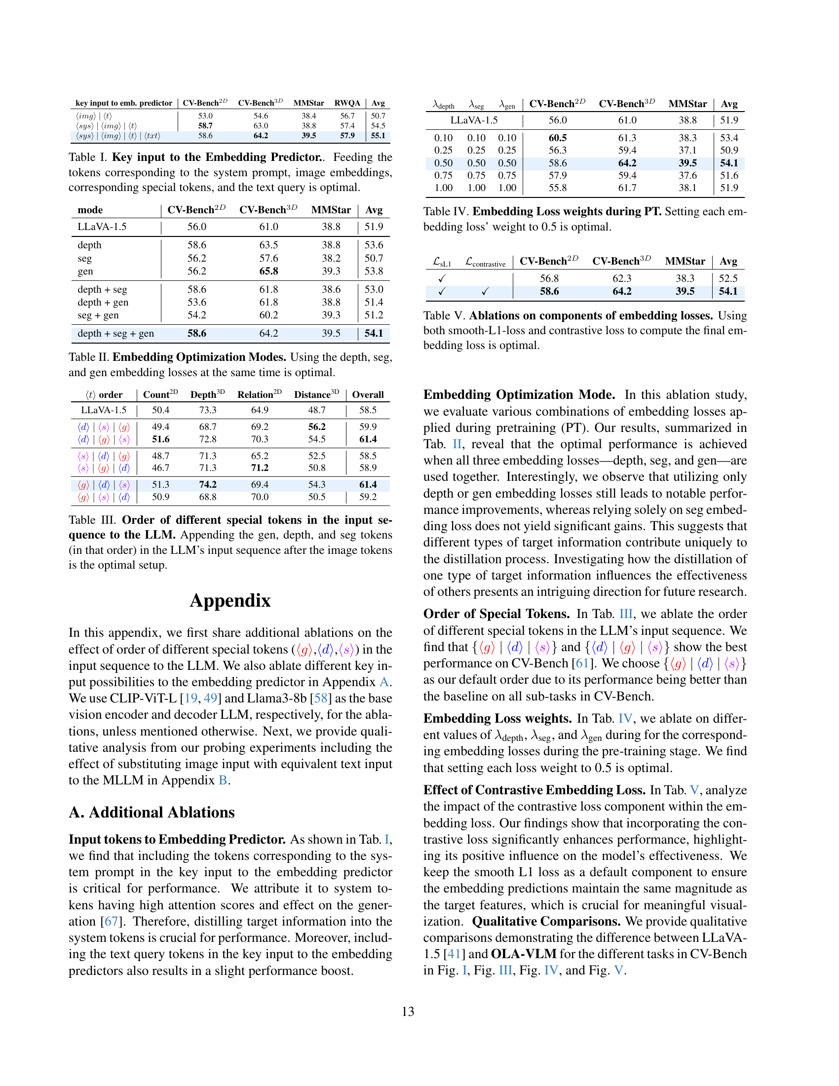
| key input to emb. predictor | CV-Bench2D | CV-Bench3D | MMStar | RWQA | Avg |
|---|---|---|---|---|---|
| ⟨img⟩ | ⟨t⟩ | 53.0 | 54.6 | 38.4 | 56.7 |
| ⟨sys⟩ | ⟨img⟩ | ⟨t⟩ | 58.7 | 63.0 | 38.8 |
| ⟨sys⟩ | ⟨img⟩ | ⟨t⟩ | ⟨txt⟩ | 58.6 | 64.2 |
🔼 This table investigates the optimal input tokens for the embedding predictor in the OLA-VLM model. The embedding predictor uses a set of learnable queries (Qtask) and a token sequence as input to generate predictions. The table explores different combinations of tokens to determine which input provides the best performance. The results show that including tokens corresponding to the system prompt, image embeddings, special tokens, and the text query yields optimal results.
read the caption
Table I: Key input to the Embedding Predictor.. Feeding the tokens corresponding to the system prompt, image embeddings, corresponding special tokens, and the text query is optimal.
| mode | CV-Bench2D | CV-Bench3D | MMStar | Avg |
|---|---|---|---|---|
| LLaVA-1.5 | 56.0 | 61.0 | 38.8 | 51.9 |
| depth | 58.6 | 63.5 | 38.8 | 53.6 |
| seg | 56.2 | 57.6 | 38.2 | 50.7 |
| gen | 56.2 | 65.8 | 39.3 | 53.8 |
| depth + seg | 58.6 | 61.8 | 38.6 | 53.0 |
| depth + gen | 53.6 | 61.8 | 38.8 | 51.4 |
| seg + gen | 54.2 | 60.2 | 39.3 | 51.2 |
| depth + seg + gen | 58.6 | 64.2 | 39.5 | 54.1 |
🔼 This table explores different combinations of embedding losses (depth, segmentation, and generation) used during the pre-training stage of the model. It investigates the impact of using these losses individually and in combination on the overall performance of the model. The results indicate that the best performance is achieved when all three types of embedding losses are used simultaneously, suggesting a synergistic effect among them in improving the model’s ability to learn and utilize visual information.
read the caption
Table II: Embedding Optimization Modes. Using the depth, seg, and gen embedding losses at the same time is optimal.
| order | Count2D | Depth3D | Relation2D | Distance3D | Overall | |
|---|---|---|---|---|---|---|
| LLaVA-1.5 | 50.4 | 73.3 | 64.9 | 48.7 | 58.5 | |
| ⟨d⟩ | ⟨s⟩ | ⟨g⟩ | 49.4 | 68.7 | 69.2 | 56.2 |
| ⟨d⟩ | ⟨g⟩ | ⟨s⟩ | 51.6 | 72.8 | 70.3 | 54.5 |
| ⟨s⟩ | ⟨d⟩ | ⟨g⟩ | 48.7 | 71.3 | 65.2 | 52.5 |
| ⟨s⟩ | ⟨g⟩ | ⟨d⟩ | 46.7 | 71.3 | 71.2 | 50.8 |
| ⟨g⟩ | ⟨d⟩ | ⟨s⟩ | 51.3 | 74.2 | 69.4 | 54.3 |
| ⟨g⟩ | ⟨s⟩ | ⟨d⟩ | 50.9 | 68.8 | 70.0 | 50.5 |
🔼 This table investigates the optimal order for appending special tokens representing image generation (gen), depth, and segmentation (seg) information to the input sequence of a large language model (LLM). The experiment modifies the order of these tokens, placing them after the image tokens. The results show that appending the tokens in the order gen, depth, seg yields the best performance.
read the caption
Table III: Order of different special tokens in the input sequence to the LLM. Appending the gen, depth, and seg tokens (in that order) in the LLM’s input sequence after the image tokens is the optimal setup.
| λ_{gen}$ | CV-Bench2D | CV-Bench3D | MMStar | Avg | ||
|---|---|---|---|---|---|---|
| LLaVA-1.5 | 56.0 | 61.0 | 38.8 | 51.9 | ||
| 0.10 | 0.10 | 0.10 | 60.5 | 61.3 | 38.3 | 53.4 |
| 0.25 | 0.25 | 0.25 | 56.3 | 59.4 | 37.1 | 50.9 |
| 0.50 | 0.50 | 0.50 | 58.6 | 64.2 | 39.5 | 54.1 |
| 0.75 | 0.75 | 0.75 | 57.9 | 59.4 | 37.6 | 51.6 |
| 1.00 | 1.00 | 1.00 | 55.8 | 61.7 | 38.1 | 51.9 |
🔼 This table presents the results of an ablation study on the weights assigned to each of the three embedding losses (depth, segmentation, and generation) during the pre-training (PT) phase of the OLA-VLM model. The study varied the weights (0.1, 0.25, 0.5, 0.75, 1.0) for each loss, and evaluated the performance on various benchmarks (CV-Bench2D, CV-Bench3D, and MMStar). The results indicate that setting the weight of each embedding loss to 0.5 yields optimal performance.
read the caption
Table IV: Embedding Loss weights during PT. Setting each embedding loss’ weight to 0.5 is optimal.
| mathcal{L}_{contrastive}$ | CV-Bench2D | CV-Bench3D | MMStar | Avg | |
|---|---|---|---|---|---|
| ✓ | 56.8 | 62.3 | 38.3 | 52.5 | |
| ✓ | ✓ | 58.6 | 64.2 | 39.5 | 54.1 |
🔼 This table presents ablation studies on the components of the embedding loss function used in the OLA-VLM model. The embedding loss combines smooth L1 loss and contrastive loss to optimize the model’s visual representation learning. The experiment varies the usage of these loss components (smooth L1 only, contrastive only, both) to determine the optimal combination for the best performance. The results show that using both smooth L1 loss and contrastive loss together leads to the best performance.
read the caption
Table V: Ablations on components of embedding losses. Using both smooth-L1-loss and contrastive loss to compute the final embedding loss is optimal.
Full paper#
