↗ arXiv ↗ Hugging Face ↗ Papers with Code
TL;DR#
Gaze target estimation, predicting where a person is looking, traditionally involves complex multi-branch models combining features from scene, head, and auxiliary sources. This complexity leads to challenges in training and scalability. Prior work often faces limitations due to reliance on small-scale datasets and computationally expensive architectures. The task is of significant interest, with applications in social interaction analysis and human-computer interaction.
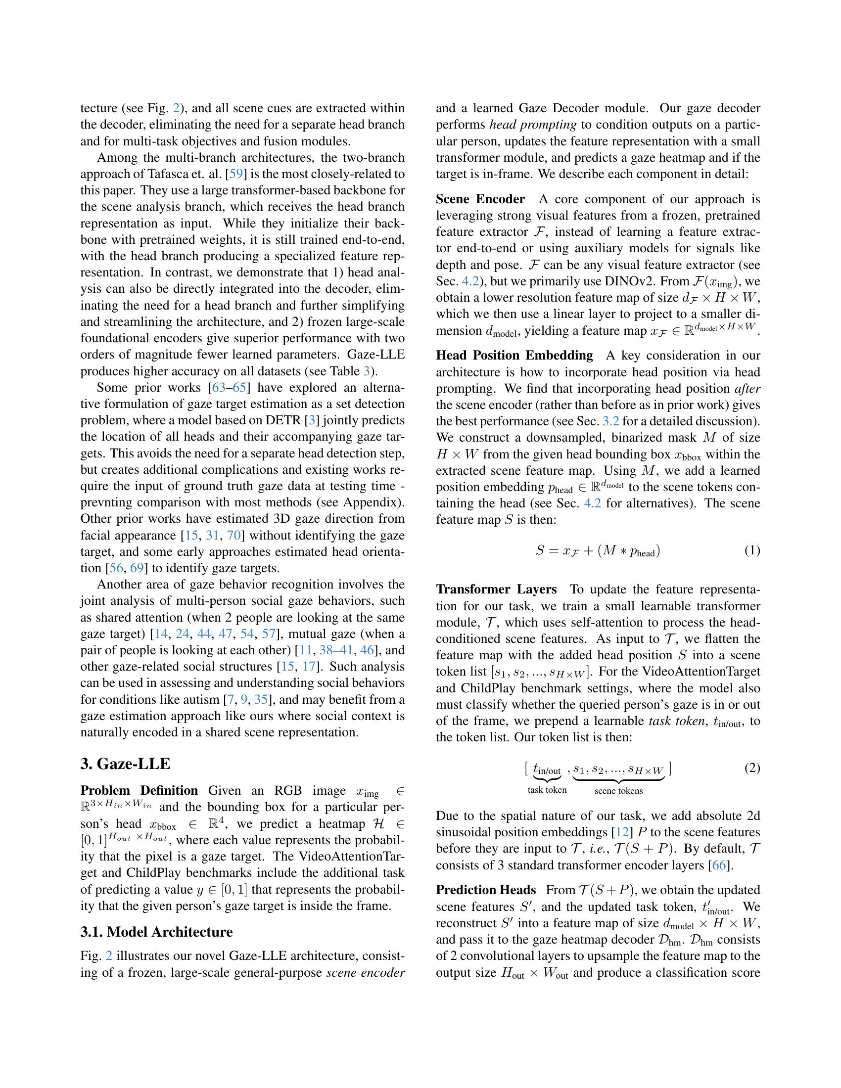
This paper introduces Gaze-LLE, a novel method that significantly simplifies this task. It leverages a pretrained DINOv2 encoder, a powerful general-purpose feature extractor, extracting a single scene representation. A person-specific positional prompt is added for the head, processed via a lightweight transformer module, and decoded for gaze prediction. Gaze-LLE achieves state-of-the-art performance with significantly fewer parameters and faster training times, demonstrating the potential of foundation models in simplifying and improving gaze estimation. This breakthrough opens doors to more efficient and scalable systems for various applications requiring gaze analysis.
Key Takeaways#
Why does it matter?#
This paper is crucial because it demonstrates the feasibility of using pre-trained large-scale models for gaze estimation, a task previously reliant on complex, hand-crafted pipelines. This approach significantly simplifies architecture, improves efficiency, and opens avenues for leveraging advancements in foundation models for improved gaze estimation, impacting human-computer interaction, social behavior analysis, and more.
Visual Insights#

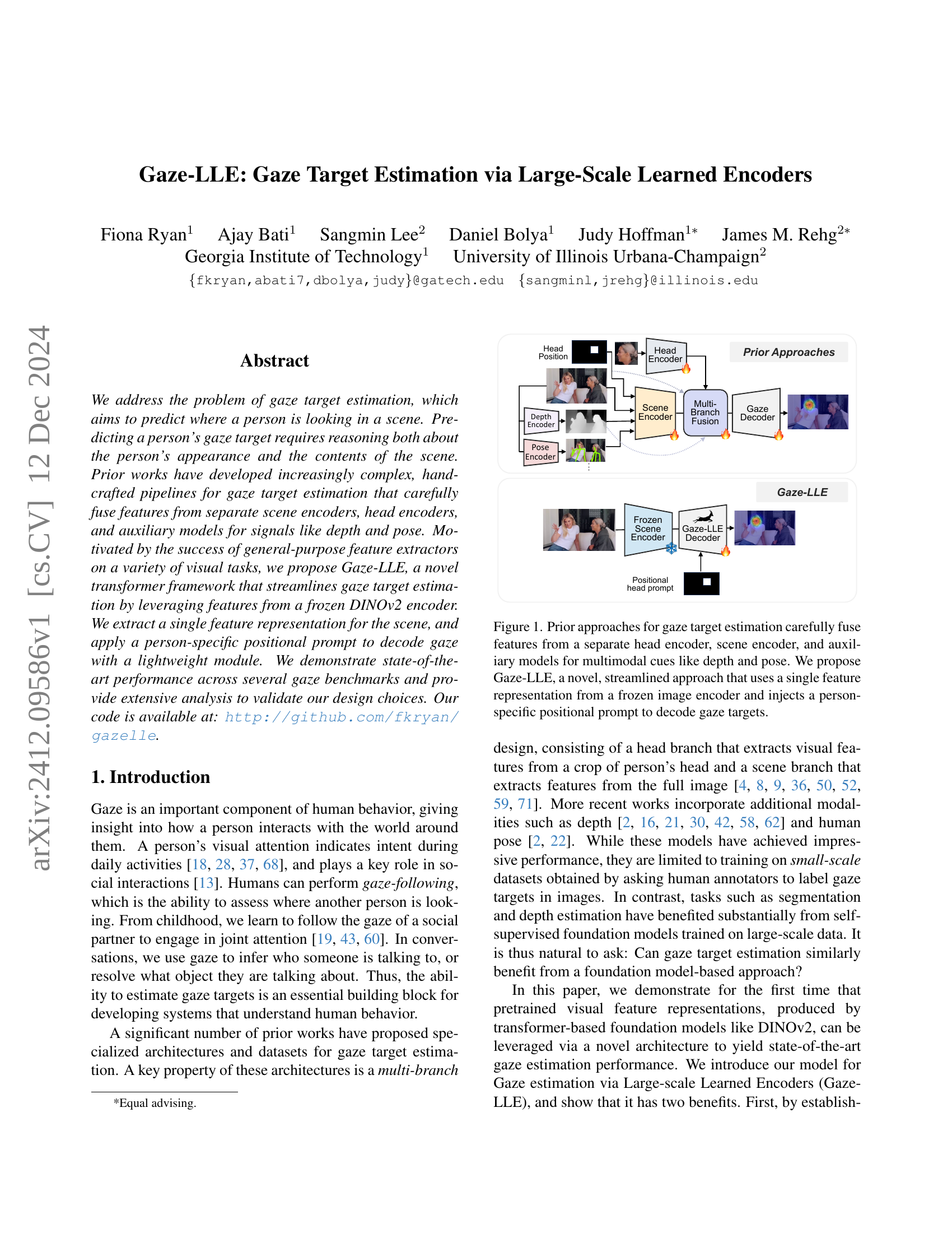
🔼 Traditional gaze estimation methods use multiple encoders (head, scene, and auxiliary encoders for depth and pose) to combine features and predict gaze targets. This figure contrasts these complex, multi-branch approaches with the proposed Gaze-LLE method. Gaze-LLE simplifies the process by using a single, frozen (pre-trained and not further updated during training) image encoder. It extracts a scene-wide feature representation and adds a person-specific positional prompt to directly decode the gaze target, eliminating the need for feature fusion from multiple encoders.
read the caption
Figure 1: Prior approaches for gaze target estimation carefully fuse features from a separate head encoder, scene encoder, and auxiliary models for multimodal cues like depth and pose. We propose Gaze-LLE, a novel, streamlined approach that uses a single feature representation from a frozen image encoder and injects a person-specific positional prompt to decode gaze targets.
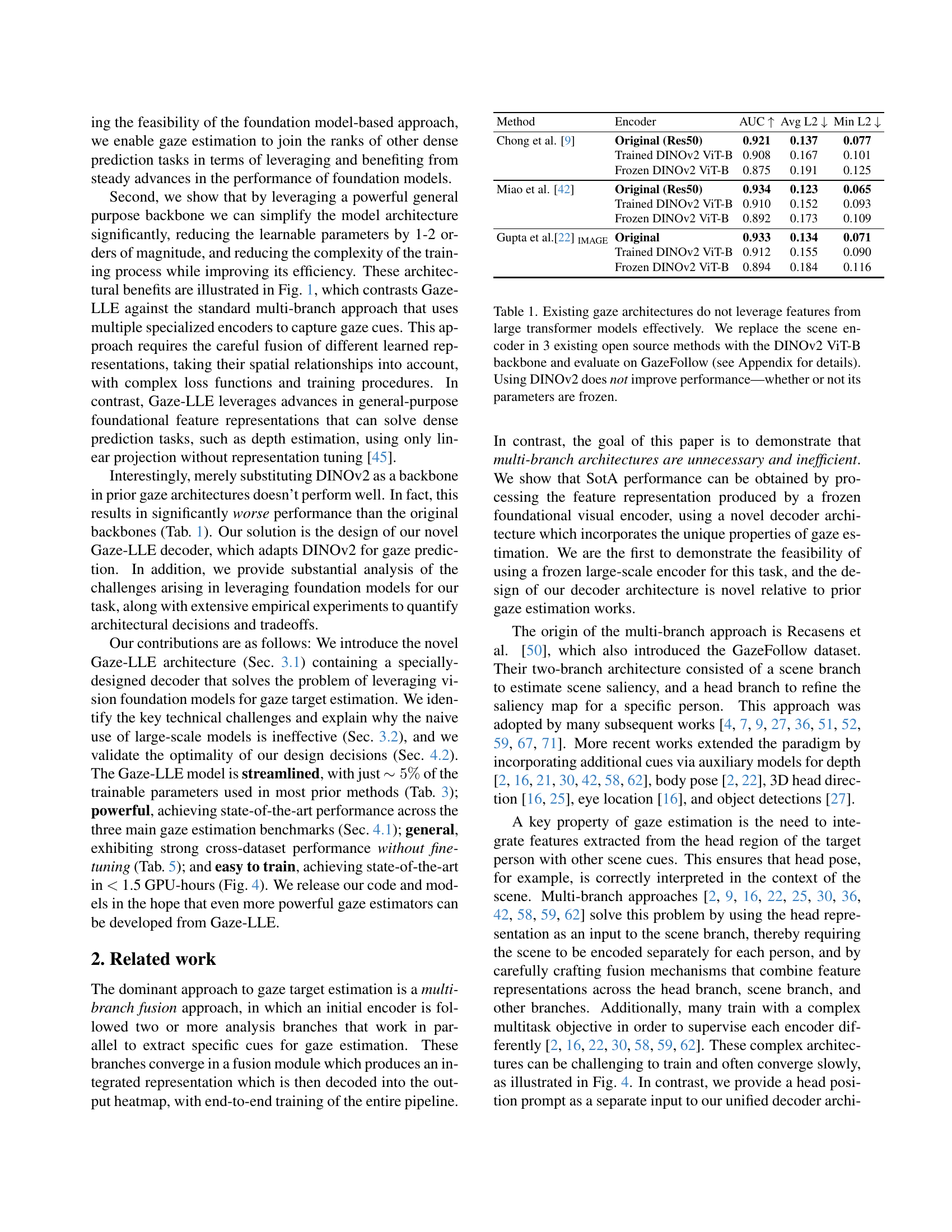
| Method | Encoder | AUC ↑ | Avg L2 ↓ | Min L2 ↓ |
|---|---|---|---|---|
| Chong et al. [9] | Original (Res50) | 0.921 | 0.137 | 0.077 |
| Trained DINOv2 ViT-B | 0.908 | 0.167 | 0.101 | |
| Frozen DINOv2 ViT-B | 0.875 | 0.191 | 0.125 | |
| Miao et al. [42] | Original (Res50) | 0.934 | 0.123 | 0.065 |
| Trained DINOv2 ViT-B | 0.910 | 0.152 | 0.093 | |
| Frozen DINOv2 ViT-B | 0.892 | 0.173 | 0.109 | |
| Gupta et al. [22] IMAGE | Original | 0.933 | 0.134 | 0.071 |
| Trained DINOv2 ViT-B | 0.912 | 0.155 | 0.090 | |
| Frozen DINOv2 ViT-B | 0.894 | 0.184 | 0.116 |
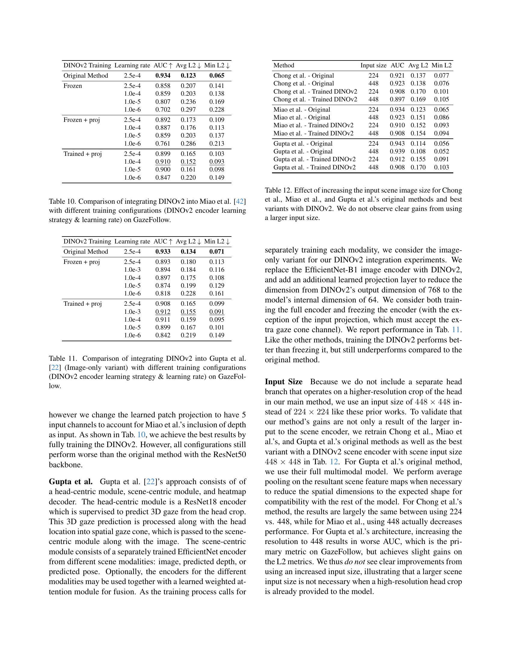
🔼 This table compares the performance of three existing gaze estimation models when using different scene encoders. The original scene encoders in each of the three models are replaced with a DINOv2 ViT-B backbone. The table shows that using the DINOv2 encoder, whether its parameters are frozen or fine-tuned, does not lead to improved performance compared to the original encoders in these models. The experiments are conducted on the GazeFollow dataset.
read the caption
Table 1: Existing gaze architectures do not leverage features from large transformer models effectively. We replace the scene encoder in 3 existing open source methods with the DINOv2 ViT-B backbone and evaluate on GazeFollow (see Appendix for details). Using DINOv2 does not improve performance—whether or not its parameters are frozen.
In-depth insights#
Foundation Model Use#
The paper explores the use of foundation models, specifically DINOv2, in gaze target estimation. A key insight is that directly substituting DINOv2 into existing multi-branch architectures proves ineffective. The authors highlight the challenges in naively applying these large models, attributing the poor performance to incompatibility between the pre-trained model and the specific task requirements. Therefore, they introduce Gaze-LLE, a novel architecture featuring a specialized decoder which adapts DINOv2’s features for accurate gaze prediction. This approach leverages the power of pre-trained representations while significantly reducing the number of trainable parameters, improving efficiency, and achieving state-of-the-art results. The study emphasizes the importance of architectural design when integrating foundation models into existing systems and suggests that a simple substitution is insufficient; careful adaptation is crucial for optimal performance.
Head Prompting#
The concept of ‘Head Prompting’ in the context of gaze estimation is a clever approach to leverage the power of large-scale learned encoders without the need for extensive, specialized training. Instead of relying on separate head and scene encoders, which increases complexity and training time, head prompting injects person-specific information directly into a shared feature representation. This injection, often in the form of a positional embedding derived from the head bounding box, acts as a conditional signal. The network effectively learns to associate this prompt with the visual features from the scene, allowing it to focus its attention and refine the gaze prediction for that specific individual. This approach significantly simplifies the architecture, reduces the number of trainable parameters, and improves efficiency while maintaining state-of-the-art performance. A key design choice appears to be the timing and method of injecting the head prompt, with the paper suggesting that injecting it after the scene encoder, as opposed to before, yields superior results. The method demonstrates the feasibility of using powerful, pretrained encoders while maintaining computational efficiency and generalizability.
Decoder Design#
The decoder design is a critical aspect of the Gaze-LLE model, significantly impacting performance. The authors opt for a streamlined design, eschewing the complex multi-branch architectures common in prior gaze estimation works. Instead of separate head and scene encoders, Gaze-LLE utilizes a single feature representation extracted from a frozen DINOv2 encoder, a powerful general-purpose backbone. This simplification dramatically reduces the number of trainable parameters, improving efficiency. The novelty lies in the introduction of ‘head prompting’, whereby a person-specific positional embedding is injected into the scene features, conditioning the decoder on the individual’s head location without the need for a separate head branch. This process leverages the backbone’s existing powerful feature representations, adapting them for the gaze estimation task using a lightweight transformer module and subsequent convolutions to generate the final heatmap. Extensive analysis validates this approach, demonstrating that the late head integration and the transformer-based decoding method achieve superior performance compared to alternative strategies, showcasing the effectiveness and elegance of the chosen design.
Cross-dataset Results#
The ‘Cross-dataset Results’ section would be crucial for evaluating the generalizability of the proposed Gaze-LLE model. A strong model should demonstrate consistent performance across various datasets, indicating its ability to generalize beyond the training data. The results would reveal whether the model’s gains are dataset-specific or represent a genuine advance in gaze estimation. Analyzing the performance metrics (AUC, L2 error) across different datasets will uncover if Gaze-LLE is robust to variations in image quality, scene complexity, and demographic characteristics. A significant drop in performance on unseen datasets would suggest overfitting or limitations in model architecture. Conversely, consistent high performance across diverse datasets would strongly support the claim that Gaze-LLE benefits from a powerful and generalizable foundation model. The extent of performance degradation will highlight limitations and point to areas for future improvement, such as incorporating domain adaptation techniques.
Future Work#
Future research directions stemming from this Gaze-LLE model could explore several promising avenues. Extending the model to handle 3D gaze estimation would enhance its practical utility, particularly in applications requiring depth perception. Investigating more sophisticated head pose handling techniques beyond simple positional prompts, perhaps incorporating learned head pose embeddings or attention mechanisms, could further improve accuracy and robustness. Exploring alternative backbone architectures, beyond DINOv2, such as those optimized for video or incorporating multimodal cues, might uncover further performance gains or enable adaptation to different data modalities. Furthermore, research into efficient inference methods for deployment on resource-constrained devices (e.g., edge devices) is crucial to make this technology widely accessible. Finally, benchmarking on more diverse and challenging datasets, representing various conditions and demographics, is essential to rigorously assess the generalizability and limitations of the approach and to drive future advancements in gaze estimation.
More visual insights#
More on figures

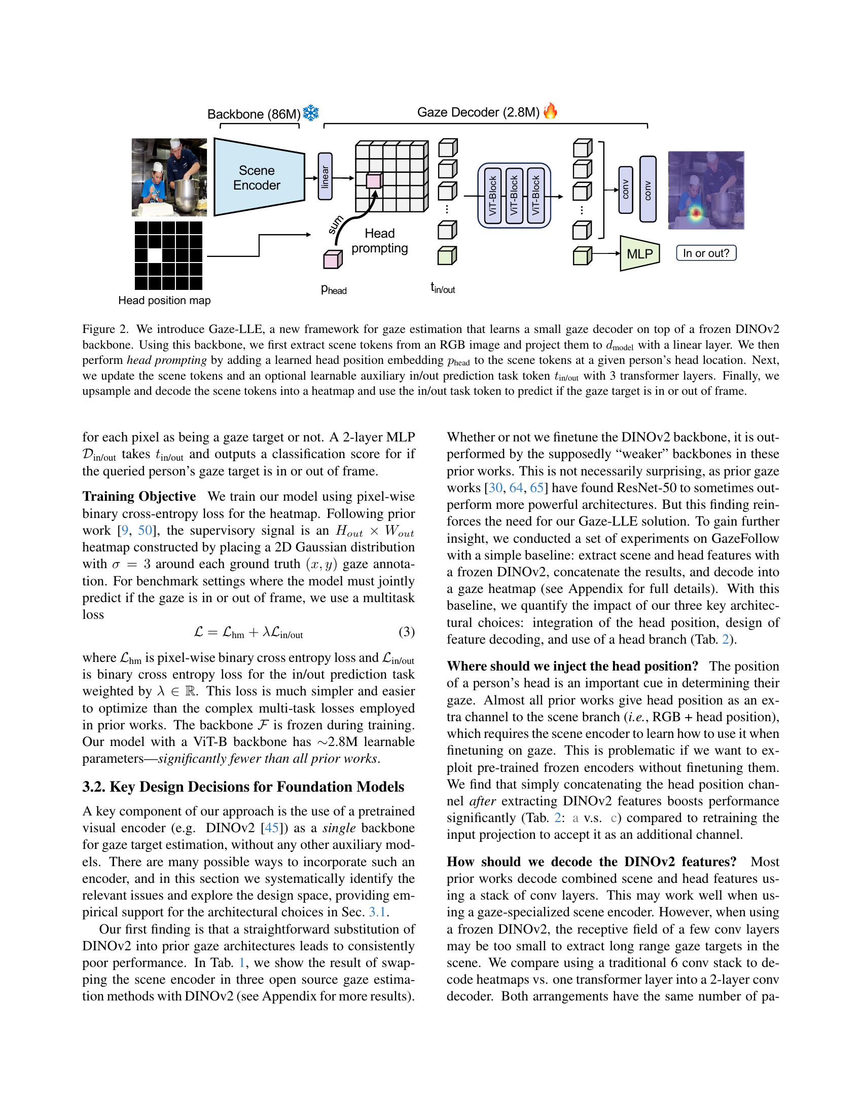
🔼 Gaze-LLE is a novel gaze estimation framework. It uses a pre-trained DINOv2 model (frozen weights) as its backbone to extract visual features from an input RGB image. These scene features are linearly projected to a lower dimension. A learned head position embedding is then added to the scene features, specifically at the location of the person’s head (obtained from a bounding box). This combined representation is then processed by three transformer layers. An optional auxiliary task token is included in the input if the task requires in/out-of-frame gaze target prediction. Finally, a lightweight decoder module upsamples the processed features and predicts a heatmap representing the gaze target location, along with the in/out classification if applicable.
read the caption
Figure 2: We introduce Gaze-LLE, a new framework for gaze estimation that learns a small gaze decoder on top of a frozen DINOv2 backbone. Using this backbone, we first extract scene tokens from an RGB image and project them to dmodelsubscript𝑑modeld_{\text{model}}italic_d start_POSTSUBSCRIPT model end_POSTSUBSCRIPT with a linear layer. We then perform head prompting by adding a learned head position embedding pheadsubscript𝑝headp_{\text{head}}italic_p start_POSTSUBSCRIPT head end_POSTSUBSCRIPT to the scene tokens at a given person’s head location. Next, we update the scene tokens and an optional learnable auxiliary in/out prediction task token tin/outsubscript𝑡in/outt_{\text{in/out}}italic_t start_POSTSUBSCRIPT in/out end_POSTSUBSCRIPT with 3 transformer layers. Finally, we upsample and decode the scene tokens into a heatmap and use the in/out task token to predict if the gaze target is in or out of frame.

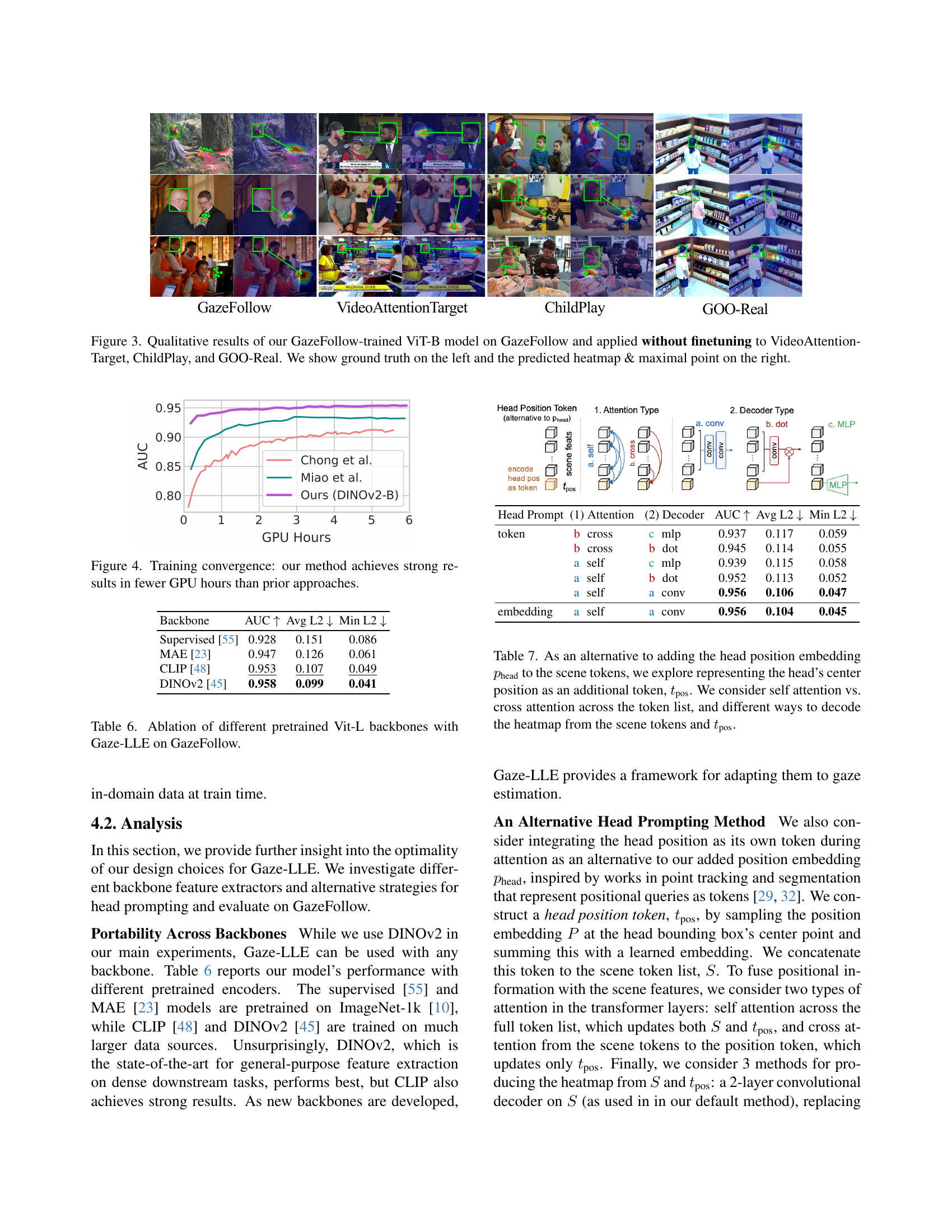
🔼 This figure shows a qualitative comparison of the Gaze-LLE model’s performance on four different datasets. The GazeFollow-trained ViT-B model is applied to GazeFollow, VideoAttentionTarget, ChildPlay, and GOO-Real datasets without any fine-tuning. For each dataset, several examples are provided. Each example shows the ground truth gaze location on the left and the model’s predicted gaze heatmap (with the maximum probability point highlighted) on the right. This visualization helps to assess the model’s ability to generalize to unseen datasets and its qualitative performance in different scenarios.
read the caption
Figure 3: Qualitative results of our GazeFollow-trained ViT-B model on GazeFollow and applied without finetuning to VideoAttentionTarget, ChildPlay, and GOO-Real. We show ground truth on the left and the predicted heatmap & maximal point on the right.

🔼 This figure shows the training convergence curves for Gaze-LLE and several state-of-the-art methods on the GazeFollow dataset. The x-axis represents training time in GPU hours, and the y-axis represents the Area Under the Curve (AUC) metric, a common evaluation metric for gaze estimation. The plot demonstrates that Gaze-LLE achieves comparable or better performance than other methods in significantly less training time, highlighting its efficiency.
read the caption
Figure 4: Training convergence: our method achieves strong results in fewer GPU hours than prior approaches.

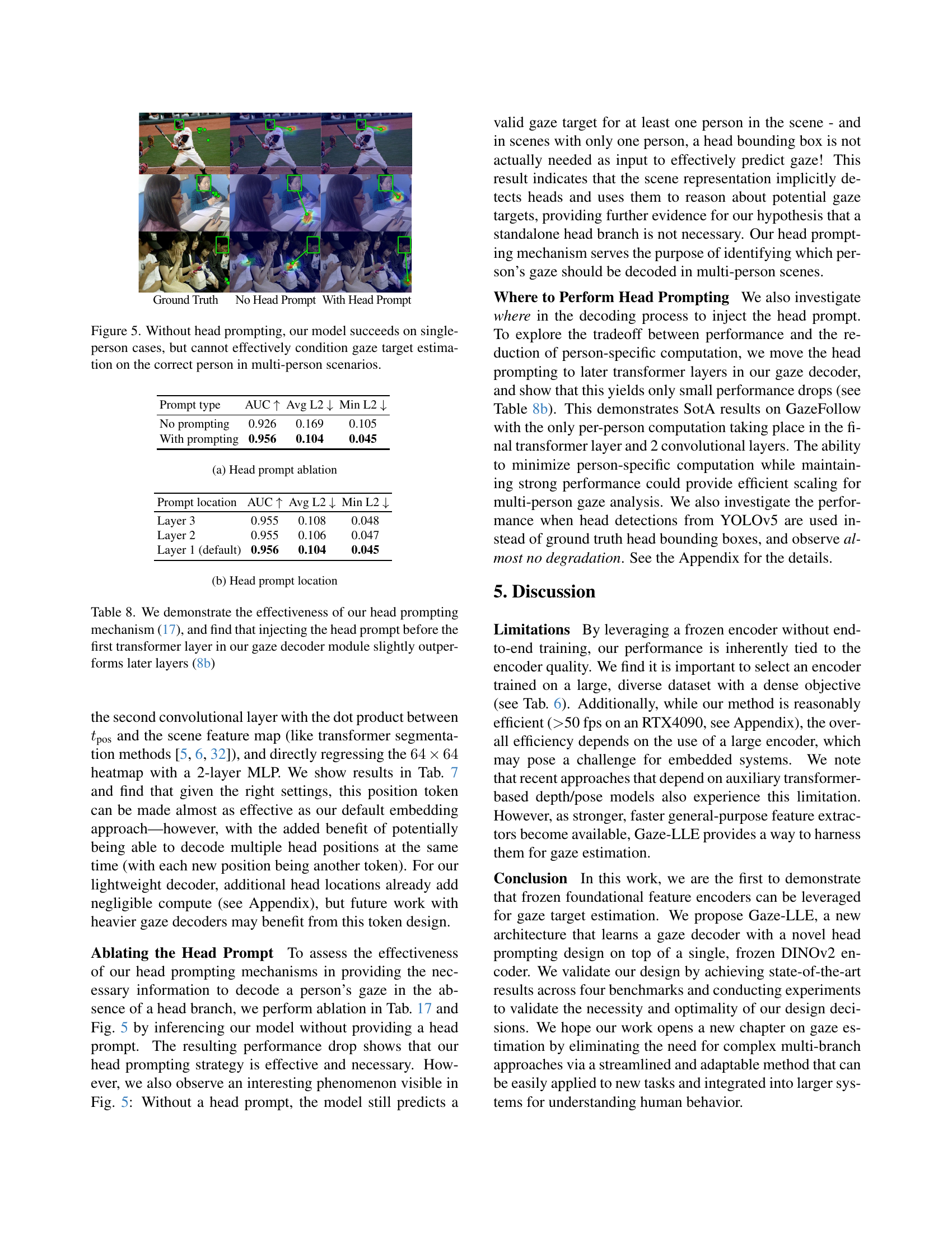
🔼 This figure demonstrates the importance of head prompting in Gaze-LLE, especially when dealing with multiple people in a scene. The leftmost column shows ground truth gaze targets. The center column shows the model’s gaze predictions without head prompting. In single-person scenes, the model generally predicts the gaze target correctly. However, when multiple people are present (as in the other two columns), the model struggles to accurately determine which person’s gaze it should estimate, resulting in inaccurate predictions. This highlights the crucial role of head prompting in disambiguating gaze targets in multi-person contexts.
read the caption
Figure 5: Without head prompting, our model succeeds on single-person cases, but cannot effectively condition gaze target estimation on the correct person in multi-person scenarios.

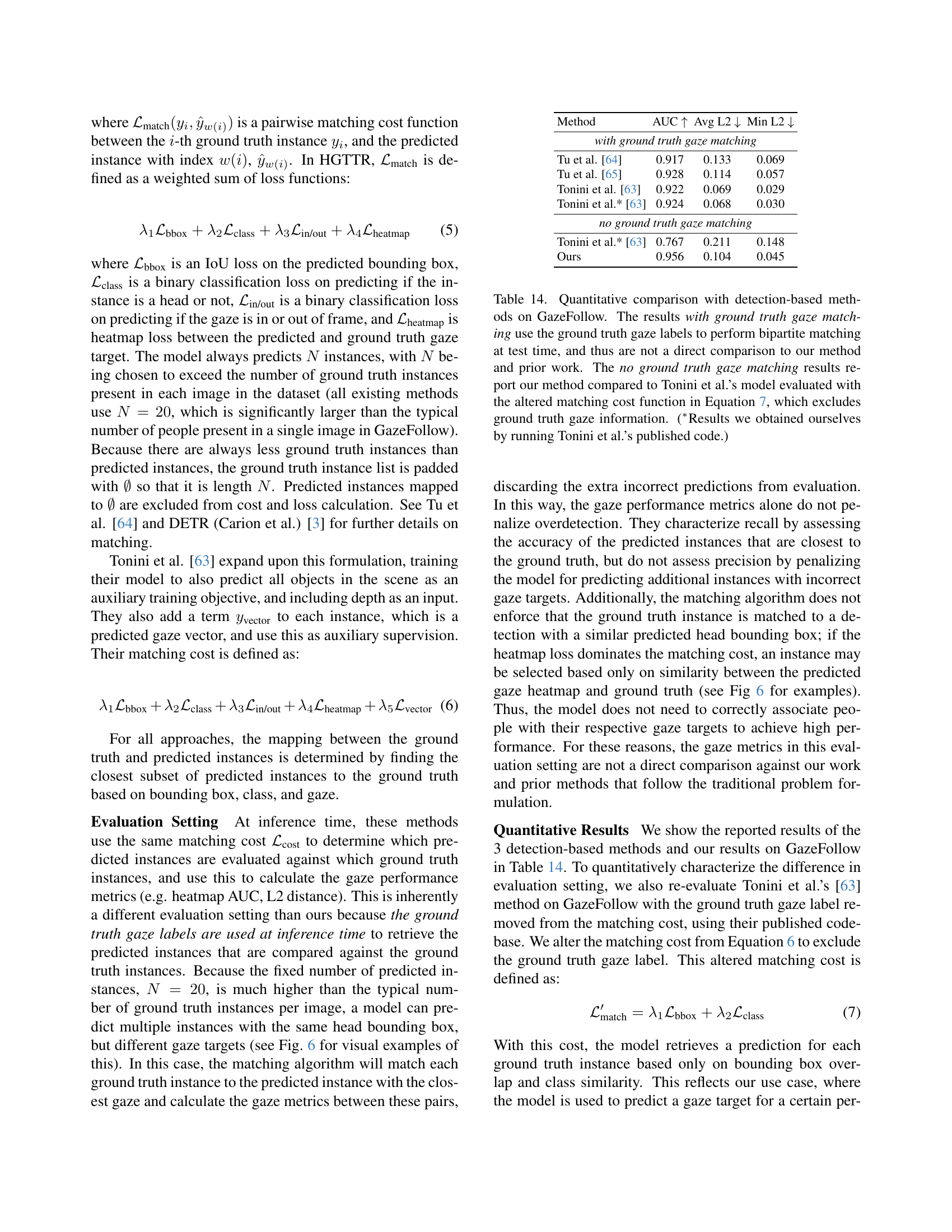
🔼 This figure compares the results of gaze estimation using two different matching algorithms: Tonini et al.’s original algorithm, which incorporates ground truth gaze information, and a modified algorithm that excludes ground truth gaze information and relies only on bounding box overlap for matching. The figure uses three examples to illustrate the differences. The first two rows highlight cases where Tonini et al.’s algorithm incorrectly associates a gaze prediction with the wrong person due to the inclusion of ground truth gaze information in the matching process. The third row shows an example of overdetection where multiple gaze predictions are made for the same person, and the algorithm selects one based on heatmap similarity. The comparison demonstrates that the absence of ground truth gaze in the matching process makes it more difficult to select the best gaze prediction when multiple predictions are present, highlighting a limitation of the detection-based approach.
read the caption
Figure 6: We show the output gaze instances (predicted head bounding box & gaze heatmap) from Tonini et al.’s model [63] for 3 examples. We identify the instances selected by Tonini et al.’s matching cost (which uses the ground truth gaze) and our altered matching cost (which excludes ground truth gaze and instead performs matching based on bounding box overlap). Tonini et al.’s matching algorithm selects the instance with the closest gaze prediction to the ground truth, but the bounding box prediction does not always correspond to the correct person (Rows 1-2). Additionally, we observe overdetection, where the algorithm predicts multiple instances for the same person with different gaze heatmaps (Row 3). Without the use of ground truth gaze information, the model cannot determine which of these instances is best.

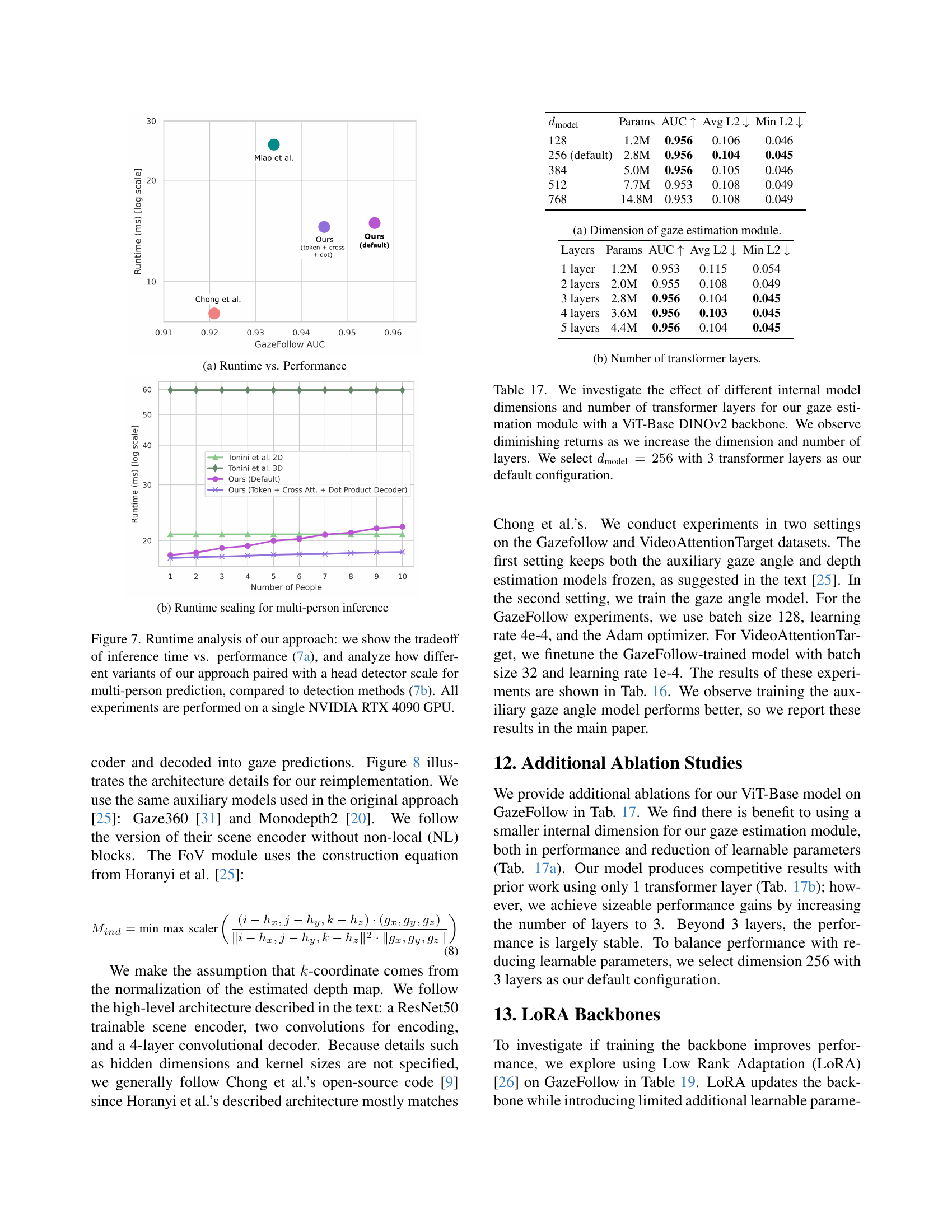
🔼 The figure shows a comparison of the inference speed and accuracy of Gaze-LLE against other state-of-the-art gaze estimation methods. It highlights that Gaze-LLE achieves significantly faster inference speed while maintaining high accuracy compared to methods using multiple branches and auxiliary models. The plot demonstrates a clear tradeoff between runtime and performance. The y-axis represents the Area Under the Curve (AUC) metric, a measure of accuracy, while the x-axis shows the inference time in milliseconds (ms) on a logarithmic scale.
read the caption
(a) Runtime vs. Performance

🔼 This figure shows how the model’s runtime scales when processing multiple people in a single image. It compares the inference time (in milliseconds) for a single person versus multiple people (1 to 10 people). Two different model configurations are tested: the default model and a modified version that employs cross-attention and dot-product decoding. This allows for an assessment of the computational efficiency of each method with increasing scene complexity.
read the caption
(b) Runtime scaling for multi-person inference

🔼 Figure 7 presents a runtime analysis comparing Gaze-LLE with other methods. Part (a) illustrates the trade-off between inference speed and performance. It shows that while Gaze-LLE is faster than some state-of-the-art methods, others achieve higher performance at the cost of speed. Part (b) explores how Gaze-LLE scales with the number of people detected in the image, which shows the model’s runtime increasing only slightly when using a single RTX 4090 GPU, even when estimating gaze for multiple individuals. This contrasts with methods using a detection-based approach.
read the caption
Figure 7: Runtime analysis of our approach: we show the tradeoff of inference time vs. performance (7(a)), and analyze how different variants of our approach paired with a head detector scale for multi-person prediction, compared to detection methods (7(b)). All experiments are performed on a single NVIDIA RTX 4090 GPU.

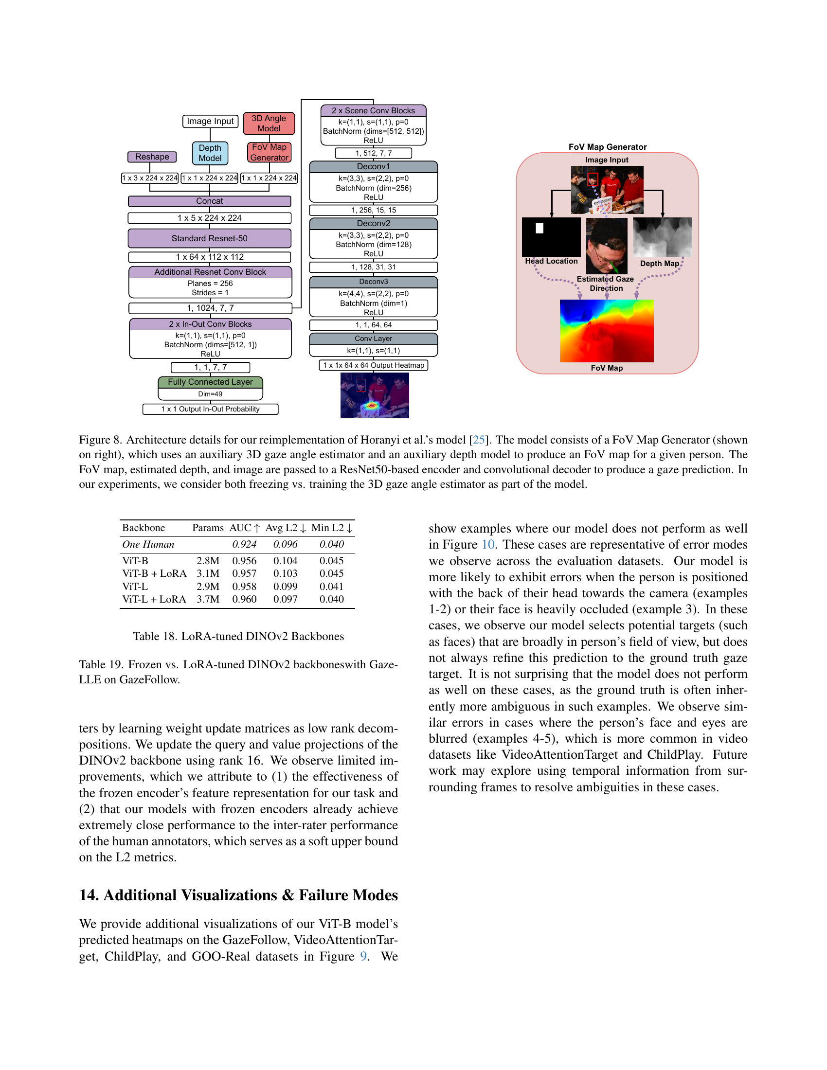
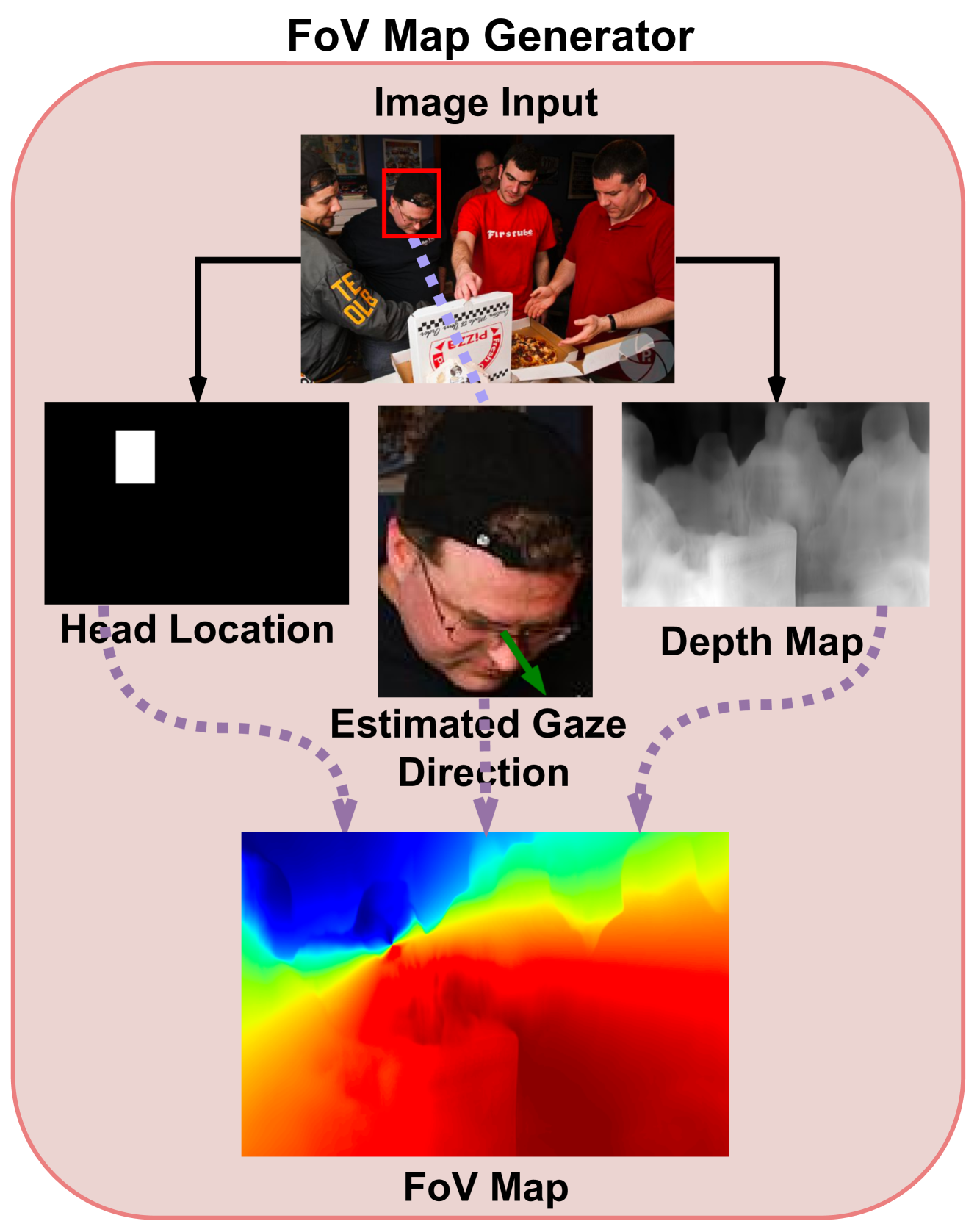
🔼 This figure details the architecture of the re-implementation of Horanyi et al.’s model for gaze estimation. It illustrates a multi-stage process. First, a FoV (Field of View) map is generated using auxiliary modules: a 3D gaze angle estimator and a depth estimation model. These provide context for gaze prediction. Then, the FoV map, the estimated depth map, and the input image are combined and fed into a ResNet50-based encoder. Features extracted by the encoder are processed by a convolutional decoder which ultimately outputs a gaze prediction. The researchers explored two experimental variations: one where the auxiliary modules are frozen (weights are not updated during training) and another where they are trained alongside the main model.
read the caption
Figure 8: Architecture details for our reimplementation of Horanyi et al.’s model [25]. The model consists of a FoV Map Generator (shown on right), which uses an auxiliary 3D gaze angle estimator and an auxiliary depth model to produce an FoV map for a given person. The FoV map, estimated depth, and image are passed to a ResNet50-based encoder and convolutional decoder to produce a gaze prediction. In our experiments, we consider both freezing vs. training the 3D gaze angle estimator as part of the model.

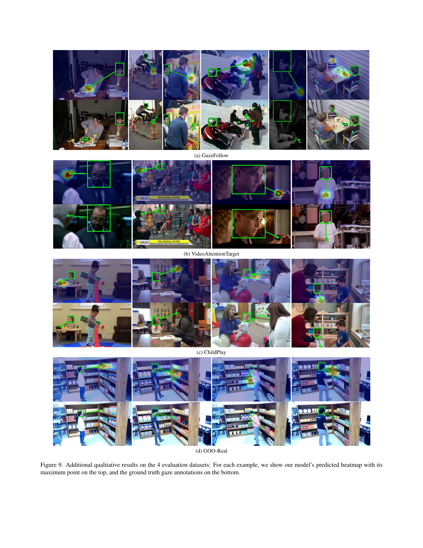
🔼 This figure shows qualitative results from the GazeFollow dataset. It displays several example images where the model’s predicted gaze heatmap is overlaid on the original image. The heatmap indicates the model’s prediction of where the person is looking, with warmer colors representing a higher probability of gaze focus. The ground truth gaze annotations are also shown for comparison.
read the caption
(a) GazeFollow
🔼 This figure shows qualitative results on the VideoAttentionTarget dataset. For each example, the model’s predicted heatmap (with its maximum point) is displayed on top, and the ground truth gaze annotations are shown at the bottom. This allows for a visual comparison of the model’s gaze prediction accuracy against the human-annotated gaze targets.
read the caption
(b) VideoAttentionTarget

🔼 This figure shows qualitative results from the ChildPlay dataset. Each example shows the model’s predicted heatmap (with its maximum point overlaid) and the ground truth gaze annotations.
read the caption
(c) ChildPlay

🔼 Figure 9(d) presents qualitative results from the GOO-Real dataset, illustrating the model’s gaze prediction performance in a retail setting. For each example, the model’s heatmap is displayed with its maximal point (predicted gaze target location), alongside the ground truth gaze annotation. GOO-Real presents a unique challenge as it involves a retail environment where the person is often not facing directly toward the camera. This figure demonstrates the model’s ability to generalize to diverse scenarios and various gaze behaviors.
read the caption
(d) GOO-Real

🔼 Figure 9 presents a qualitative analysis of the Gaze-LLE model’s performance across four datasets: GazeFollow, VideoAttentionTarget, ChildPlay, and GOO-Real. For each dataset, several example images are shown, each displaying a comparison between the model’s predicted gaze heatmap (with the maximum activation point highlighted) and the corresponding ground truth gaze annotation. This visual comparison helps to assess the model’s accuracy and identify potential failure cases.
read the caption
Figure 9: Additional qualitative results on the 4 evaluation datasets: For each example, we show our model’s predicted heatmap with its maximum point on the top, and the ground truth gaze annotations on the bottom.

🔼 This figure showcases instances where the Gaze-LLE model struggles to accurately predict gaze targets. These failure cases highlight the model’s limitations when dealing with specific visual challenges. Examples 1 and 2 illustrate scenarios where the person’s head is turned away from the camera, making it difficult to determine their gaze direction. Example 3 presents a situation where the head is occluded, hindering the model’s ability to process relevant visual cues. Finally, examples 4 and 5 depict situations with blurred faces, leading to inaccurate gaze estimations. These examples demonstrate the model’s sensitivity to factors such as head orientation, occlusion, and image clarity, which can affect the reliability of gaze prediction.
read the caption
Figure 10: Lower performing cases: we observe errors in some cases where the head is facing away from the camera (examples 1-2), the head is occluded (examples 3), or the face is blurred (examples 4-5).
More on tables
| (1) Head Integration | (2) Decoder | (3) Branches | GazeFollow AUC ↑ | GazeFollow Avg L2 ↓ | GazeFollow Min L2 ↓ | |
|---|---|---|---|---|---|---|
| a. | early | conv | H+S | 0.854 | 0.254 | 0.168 |
| b. | early | tran | H+S | 0.904 | 0.178 | 0.113 |
| c. | late | conv | H+S | 0.932 | 0.155 | 0.089 |
| d. | late | tran | H+S | 0.954 | 0.113 | 0.053 |
| e. | late | conv | S | 0.916 | 0.184 | 0.115 |
| f. | late | tran | S | 0.953 | 0.114 | 0.054 |
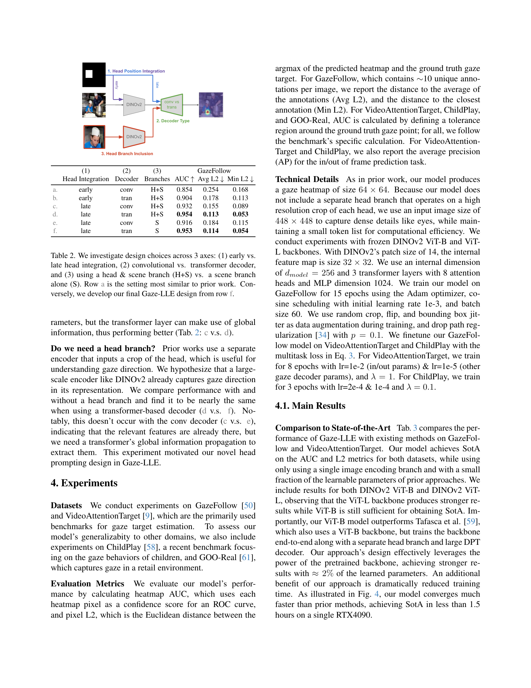
🔼 This table presents an ablation study analyzing the impact of different architectural design choices on gaze estimation performance. Three key design aspects are examined: the timing of head integration (early vs. late), the type of decoder used (convolutional vs. transformer), and whether the model uses a separate head branch or just a scene branch. Row ‘a’ represents an architecture similar to existing methods, while row ‘f’ describes the final Gaze-LLE model architecture. The results highlight the effectiveness of the choices made in the final model.
read the caption
Table 2: We investigate design choices across 3 axes: (1) early vs. late head integration, (2) convolutional vs. transformer decoder, and (3) using a head & scene branch (H+S) vs. a scene branch alone (S). Row a is the setting most similar to prior work. Conversely, we develop our final Gaze-LLE design from row f.
| Method | Learnable Params | Input | GazeFollow AUC ↑ | GazeFollow Avg L2 ↓ | GazeFollow Min L2 ↓ | VideoAttentionTarget AUC ↑ | VideoAttentionTarget L2 ↓ | VideoAttentionTarget AP ↑ |
|---|---|---|---|---|---|---|---|---|
| One Human | 0.924 | 0.096 | 0.040 | 0.921 | 0.051 | 0.925 | ||
| Recasens et al. [50] | 50M* | I | 0.878 | 0.19 | 0.113 | - | - | - |
| Chong et al. [8] | 51M* | I | 0.896 | 0.187 | 0.112 | 0.833 | 0.171 | 0.712 |
| Lian et al. [36] | 55M | I | 0.906 | 0.145 | 0.081 | - | - | - |
| Chong et al. [9] | 61M | I | 0.921 | 0.137 | 0.077 | 0.860 | 0.134 | 0.853 |
| Chen et al. [4] | 50M* | I | 0.908 | 0.136 | 0.074 | - | - | - |
| Fang et al. [16] | 68M | I+D+E | 0.922 | 0.124 | 0.067 | 0.905 | 0.108 | 0.896 |
| Bao et al. [2] | 29M* | I+D+P | 0.928 | 0.122 | - | 0.885 | 0.120 | 0.869 |
| Jin et al. [30] | >52M* | I+D+P | 0.920 | 0.118 | 0.063 | 0.900 | 0.104 | 0.895 |
| Tonini et al. [62] | 92M | I+D | 0.927 | 0.141 | - | 0.862‡ | 0.125 | 0.742 |
| Hu et al. [27] | >61M* | I+D+O | 0.923 | 0.128 | 0.069 | 0.880 | 0.118 | 0.881 |
| Gupta et al. [22] | 35M | I+D+P | 0.943 | 0.114 | 0.056 | 0.914 | 0.110 | 0.879 |
| Horanyi et al. [25]† | 46M† | I+D | 0.896† | 0.196† | 0.127† | 0.832† | 0.199† | 0.800† |
| Miao et al. [42] | 61M | I+D | 0.934 | 0.123 | 0.065 | 0.917 | 0.109 | 0.908 |
| Tafasca et al. [58] | >25M* | I+D | 0.939 | 0.122 | 0.062 | 0.914 | 0.109 | 0.834 |
| Tafasca et al. [59] | >135M* | I | 0.944 | 0.113 | 0.057 | - | 0.107 | 0.891 |
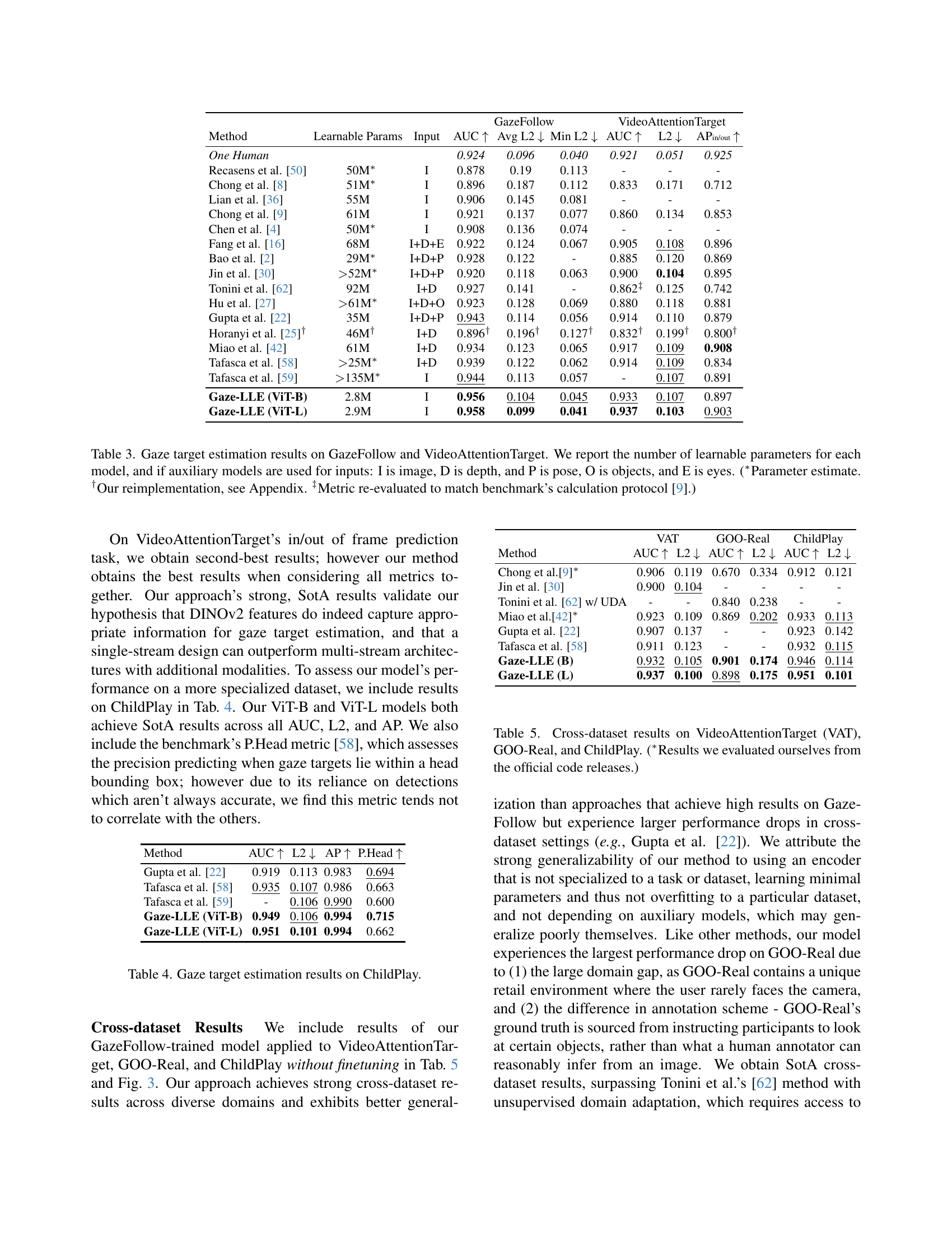
| Gaze-LLE (ViT-B) | 2.8M | I | 0.956 | 0.104 | 0.045 | 0.933 | 0.107 | 0.897 |
| Gaze-LLE (ViT-L) | 2.9M | I | 0.958 | 0.099 | 0.041 | 0.937 | 0.103 | 0.903 |
🔼 This table presents a comparison of different methods for gaze target estimation on two benchmark datasets: GazeFollow and VideoAttentionTarget. For each method, it shows the number of trainable parameters, the input data used (image (I), depth (D), pose (P), objects (O), and eyes (E)), and the performance metrics achieved: Area Under the Curve (AUC), Average L2 error, and Minimum L2 error. AUC measures the accuracy of the heatmap produced by the model, while L2 error measures the distance between the predicted gaze target and the ground truth. The table highlights the relatively small number of parameters in the proposed Gaze-LLE model compared to existing methods. Notes clarify that some parameter counts are estimates, one entry is based on a reimplementation of a prior model, and one metric was recalculated to match the methodology of a specific prior publication.
read the caption
Table 3: Gaze target estimation results on GazeFollow and VideoAttentionTarget. We report the number of learnable parameters for each model, and if auxiliary models are used for inputs: I is image, D is depth, and P is pose, O is objects, and E is eyes. (∗Parameter estimate. †Our reimplementation, see Appendix. ‡Metric re-evaluated to match benchmark’s calculation protocol [9].)
| Method | AUC ↑ | L2 ↓ | AP ↑ | P.Head ↑ |
|---|---|---|---|---|
| Gupta et al. [22] | 0.919 | 0.113 | 0.983 | 0.694 |
| Tafasca et al. [58] | 0.935 | 0.107 | 0.986 | 0.663 |
| Tafasca et al. [59] | - | 0.106 | 0.990 | 0.600 |
| Gaze-LLE (ViT-B) | 0.949 | 0.106 | 0.994 | 0.715 |
| Gaze-LLE (ViT-L) | 0.951 | 0.101 | 0.994 | 0.662 |
🔼 This table presents a comparison of different methods for gaze target estimation on the ChildPlay dataset. It shows the Area Under the Curve (AUC) of the receiver operating characteristic (ROC) curve, the average L2 distance (Avg L2), the minimum L2 distance (Min L2), and the precision of head prediction (P.Head) for each method. The ChildPlay dataset is a benchmark dataset specifically designed for evaluating gaze estimation models’ performance on the gaze behavior of children. The metrics provide a comprehensive evaluation of the accuracy and precision of gaze prediction methods on this challenging dataset.
read the caption
Table 4: Gaze target estimation results on ChildPlay.
| Method | VAT AUC ↑ | VAT L2 ↓ | GOO-Real AUC ↑ | GOO-Real L2 ↓ | ChildPlay AUC ↑ | ChildPlay L2 ↓ |
|---|---|---|---|---|---|---|
| Chong et al. [9]∗ | 0.906 | 0.119 | 0.670 | 0.334 | 0.912 | 0.121 |
| Jin et al. [30] | 0.900 | 0.104 | - | - | - | - |
| Tonini et al. [62] w/ UDA | - | - | 0.840 | 0.238 | - | - |
| Miao et al. [42]∗ | 0.923 | 0.109 | 0.869 | 0.202 | 0.933 | 0.113 |
| Gupta et al. [22] | 0.907 | 0.137 | - | - | 0.923 | 0.142 |
| Tafasca et al. [58] | 0.911 | 0.123 | - | - | 0.932 | 0.115 |
| Gaze-LLE (B) | 0.932 | 0.105 | 0.901 | 0.174 | 0.946 | 0.114 |
| Gaze-LLE (L) | 0.937 | 0.100 | 0.898 | 0.175 | 0.951 | 0.101 |
🔼 This table presents the cross-dataset generalization performance of the Gaze-LLE model. It shows the Area Under the ROC Curve (AUC) and average L2 distance metrics for the model trained only on the GazeFollow dataset, but tested on three other datasets: VideoAttentionTarget, GOO-Real, and ChildPlay. The results demonstrate the model’s ability to generalize to new, unseen datasets without requiring any fine-tuning.
read the caption
Table 5: Cross-dataset results on VideoAttentionTarget (VAT), GOO-Real, and ChildPlay. (∗Results we evaluated ourselves from the official code releases.)
| Backbone | AUC ↑ | Avg L2 ↓ | Min L2 ↓ |
|---|---|---|---|
| Supervised [55] | 0.928 | 0.151 | 0.086 |
| MAE [23] | 0.947 | 0.126 | 0.061 |
| CLIP [48] | 0.953 | 0.107 | 0.049 |
| DINOv2 [45] | 0.958 | 0.099 | 0.041 |
🔼 This table presents an ablation study evaluating the impact of different pre-trained ViT-L backbones on the performance of the Gaze-LLE model. It shows how using different pre-trained models (Supervised, MAE, CLIP, and DINOv2) as the backbone for Gaze-LLE affects performance on the GazeFollow dataset, as measured by AUC, Avg L2, and Min L2.
read the caption
Table 6: Ablation of different pretrained Vit-L backbones with Gaze-LLE on GazeFollow.
| Head Prompt | (1) Attention | (2) Decoder | AUC ↑ | Avg L2 ↓ | Min L2 ↓ |
|---|---|---|---|---|---|
| token | (b) cross | (c) mlp | 0.937 | 0.117 | 0.059 |
| (b) cross | (b) dot | 0.945 | 0.114 | 0.055 | |
| (a) self | (c) mlp | 0.939 | 0.115 | 0.058 | |
| (a) self | (b) dot | 0.952 | 0.113 | 0.052 | |
| (a) self | (a) conv | 0.956 | 0.106 | 0.047 | |
| embedding | (a) self | (a) conv | 0.956 | 0.104 | 0.045 |
🔼 This table explores alternative methods for incorporating head position information into the Gaze-LLE model. Instead of adding a learned head position embedding to the scene features, the head’s center position is represented as an additional token. The experiment compares different attention mechanisms (self-attention vs. cross-attention) applied to this modified token list, and also assesses the impact of various decoding methods on the final gaze heatmap prediction. The goal is to determine the effectiveness of representing head position information as a separate token compared to the original method which directly adds head position embedding to the scene features.
read the caption
Table 7: As an alternative to adding the head position embedding pheadsubscript𝑝headp_{\text{head}}italic_p start_POSTSUBSCRIPT head end_POSTSUBSCRIPT to the scene tokens, we explore representing the head’s center position as an additional token, tpossubscript𝑡post_{\text{pos}}italic_t start_POSTSUBSCRIPT pos end_POSTSUBSCRIPT. We consider self attention vs. cross attention across the token list, and different ways to decode the heatmap from the scene tokens and tpossubscript𝑡post_{\text{pos}}italic_t start_POSTSUBSCRIPT pos end_POSTSUBSCRIPT.
| Prompt type | AUC ↑ | Avg L2 ↓ | Min L2 ↓ |
|---|---|---|---|
| No prompting | 0.926 | 0.169 | 0.105 |
| With prompting | 0.956 | 0.104 | 0.045 |
🔼 This table presents an ablation study on the head prompt mechanism within the Gaze-LLE model. It shows the impact of removing the head prompt entirely and explores the effect of injecting the head prompt into different layers of the gaze decoder. The results quantify the effectiveness of head prompting for gaze estimation performance.
read the caption
(a) Head prompt ablation
| Prompt location | AUC ↑ | Avg L2 ↓ | Min L2 ↓ |
|---|---|---|---|
| Layer 3 | 0.955 | 0.108 | 0.048 |
| Layer 2 | 0.955 | 0.106 | 0.047 |
| Layer 1 (default) | 0.956 | 0.104 | 0.045 |
🔼 This table presents ablation study results on the impact of head prompt placement within the Gaze-LLE decoder. It shows the performance (AUC, Avg L2, Min L2) when the head prompt is injected at different transformer layers (Layer 1, Layer 2, Layer 3). The results help determine the optimal layer for head prompt integration to achieve the best balance between model performance and computational efficiency.
read the caption
(b) Head prompt location
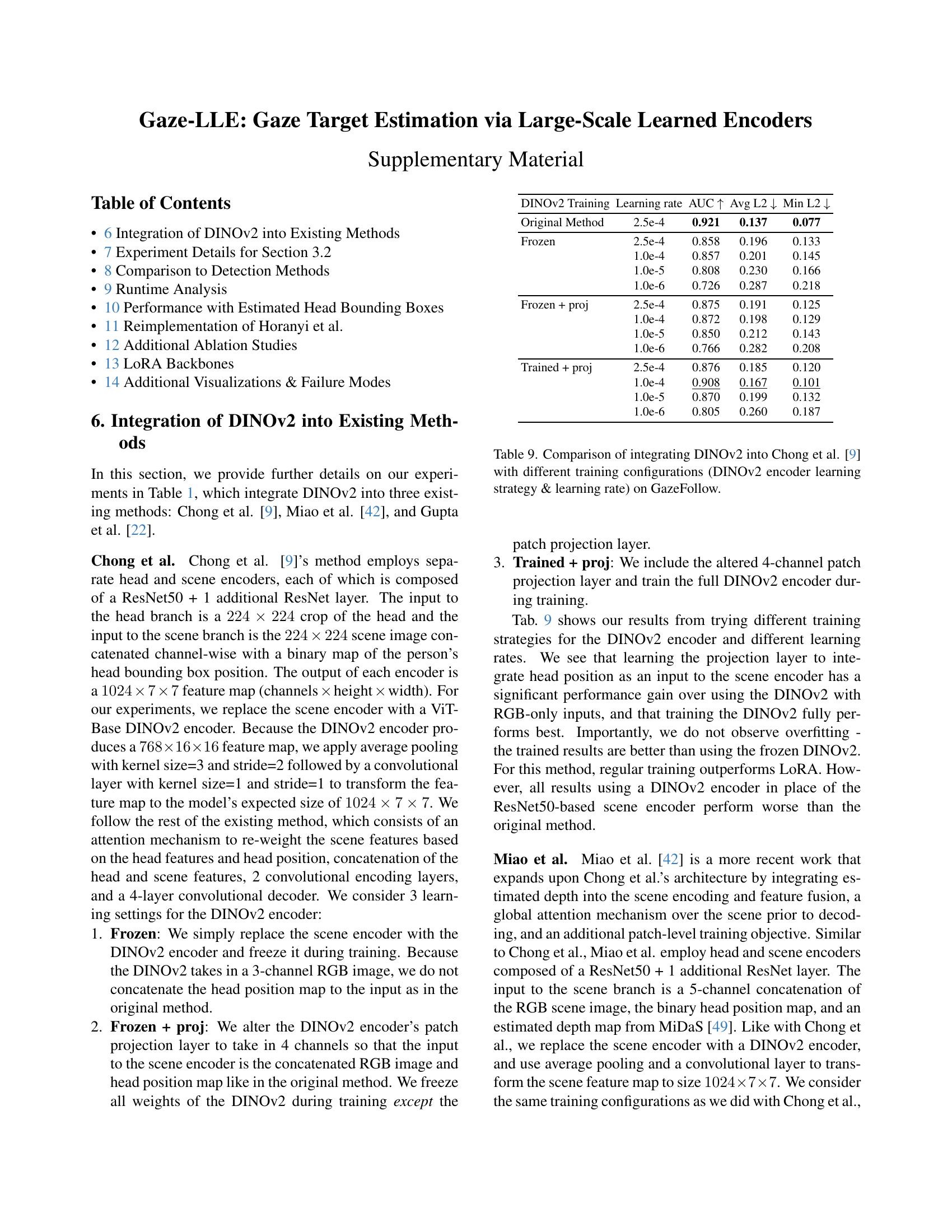
| DINOv2 Training | Learning rate | AUC ↑ | Avg L2 ↓ | Min L2 ↓ |
|---|---|---|---|---|
| Original Method | 2.5e-4 | 0.921 | 0.137 | 0.077 |
| Frozen | 2.5e-4 | 0.858 | 0.196 | 0.133 |
| 1.0e-4 | 0.857 | 0.201 | 0.145 | |
| 1.0e-5 | 0.808 | 0.230 | 0.166 | |
| 1.0e-6 | 0.726 | 0.287 | 0.218 | |
| Frozen + proj | 2.5e-4 | 0.875 | 0.191 | 0.125 |
| 1.0e-4 | 0.872 | 0.198 | 0.129 | |
| 1.0e-5 | 0.850 | 0.212 | 0.143 | |
| 1.0e-6 | 0.766 | 0.282 | 0.208 | |
| Trained + proj | 2.5e-4 | 0.876 | 0.185 | 0.120 |
| 1.0e-4 | 0.908 | 0.167 | 0.101 | |
| 1.0e-5 | 0.870 | 0.199 | 0.132 | |
| 1.0e-6 | 0.805 | 0.260 | 0.187 |
🔼 This table presents an ablation study on the head prompt’s effectiveness and placement within the Gaze-LLE model. It shows that adding a head prompt improves gaze estimation accuracy. Furthermore, it compares placing the head prompt before different transformer layers in the decoder, demonstrating that injecting it before the first layer yields slightly better results than injecting it later. The metrics used are Area Under the Curve (AUC), Average L2 distance, and Minimum L2 distance, all commonly used to evaluate gaze estimation performance.
read the caption
Table 8: We demonstrate the effectiveness of our head prompting mechanism (17), and find that injecting the head prompt before the first transformer layer in our gaze decoder module slightly outperforms later layers (8(b))
| DINOv2 Training | Learning rate | AUC ↑ | Avg L2 ↓ | Min L2 ↓ |
|---|---|---|---|---|
| Original Method | 2.5e-4 | 0.934 | 0.123 | 0.065 |
| Frozen | 2.5e-4 | 0.858 | 0.207 | 0.141 |
| 1.0e-4 | 0.859 | 0.203 | 0.138 | |
| 1.0e-5 | 0.807 | 0.236 | 0.169 | |
| 1.0e-6 | 0.702 | 0.297 | 0.228 | |
| Frozen + proj | 2.5e-4 | 0.892 | 0.173 | 0.109 |
| 1.0e-4 | 0.887 | 0.176 | 0.113 | |
| 1.0e-5 | 0.859 | 0.203 | 0.137 | |
| 1.0e-6 | 0.761 | 0.286 | 0.213 | |
| Trained + proj | 2.5e-4 | 0.899 | 0.165 | 0.103 |
| 1.0e-4 | 0.910 | 0.152 | 0.093 | |
| 1.0e-5 | 0.900 | 0.161 | 0.098 | |
| 1.0e-6 | 0.847 | 0.220 | 0.149 |
🔼 This table presents a comparison of different training strategies for integrating a pre-trained DINOv2 model into Chong et al.’s gaze estimation method. It explores the effects of freezing the DINOv2 encoder’s weights (Frozen), only training a projection layer to handle a four-channel input including head pose (Frozen + proj), and training the entire DINOv2 encoder (Trained + proj). The results, evaluated on the GazeFollow dataset, show the performance (AUC, Avg L2, Min L2) achieved with each configuration and different learning rates for the DINOv2 encoder.
read the caption
Table 9: Comparison of integrating DINOv2 into Chong et al. [9] with different training configurations (DINOv2 encoder learning strategy & learning rate) on GazeFollow.
| DINOv2 Training | Learning rate | AUC ↑ | Avg L2 ↓ | Min L2 ↓ |
|---|---|---|---|---|
| Original Method | 2.5e-4 | 0.933 | 0.134 | 0.071 |
| Frozen + proj | 2.5e-4 | 0.893 | 0.180 | 0.113 |
| 1.0e-3 | 0.894 | 0.184 | 0.116 | |
| 1.0e-4 | 0.897 | 0.175 | 0.108 | |
| 1.0e-5 | 0.874 | 0.199 | 0.129 | |
| 1.0e-6 | 0.818 | 0.228 | 0.161 | |
| Trained + proj | 2.5e-4 | 0.908 | 0.165 | 0.099 |
| 1.0e-3 | 0.912 | 0.155 | 0.091 | |
| 1.0e-4 | 0.911 | 0.159 | 0.095 | |
| 1.0e-5 | 0.899 | 0.167 | 0.101 | |
| 1.0e-6 | 0.842 | 0.219 | 0.149 |
🔼 This table presents the results of experiments integrating the DINOv2 model into Miao et al.’s [42] gaze estimation method. It investigates the impact of different training strategies for DINOv2, varying the encoder’s learning approach (frozen, frozen with a projection layer added, and fully trained) and the learning rate. The performance is evaluated on the GazeFollow dataset using AUC, average L2 distance, and minimum L2 distance metrics. The table helps to analyze the effectiveness of different DINOv2 training configurations within the broader context of Miao et al.’s method.
read the caption
Table 10: Comparison of integrating DINOv2 into Miao et al. [42] with different training configurations (DINOv2 encoder learning strategy & learning rate) on GazeFollow.
| Method | Input size | AUC | Avg L2 | Min L2 |
|---|---|---|---|---|
| Chong et al. - Original | 224 | 0.921 | 0.137 | 0.077 |
| Chong et al. - Original | 448 | 0.923 | 0.138 | 0.076 |
| Chong et al. - Trained DINOv2 | 224 | 0.908 | 0.170 | 0.101 |
| Chong et al. - Trained DINOv2 | 448 | 0.897 | 0.169 | 0.105 |
| Miao et al. - Original | 224 | 0.934 | 0.123 | 0.065 |
| Miao et al. - Original | 448 | 0.923 | 0.151 | 0.086 |
| Miao et al. - Trained DINOv2 | 224 | 0.910 | 0.152 | 0.093 |
| Miao et al. - Trained DINOv2 | 448 | 0.908 | 0.154 | 0.094 |
| Gupta et al. - Original | 224 | 0.943 | 0.114 | 0.056 |
| Gupta et al. - Original | 448 | 0.939 | 0.108 | 0.052 |
| Gupta et al. - Trained DINOv2 | 224 | 0.912 | 0.155 | 0.091 |
| Gupta et al. - Trained DINOv2 | 448 | 0.908 | 0.170 | 0.103 |
🔼 This table presents the results of experiments integrating a pre-trained DINOv2 model into the image-only variant of Gupta et al.’s [22] gaze estimation method. Different training configurations were tested: the DINOv2 encoder was either frozen, or partially trained (only the projection layer), or fully trained. Each configuration was evaluated at different learning rates, showing the impact of these choices on the performance of the gaze estimation model, measured by AUC, Avg L2, and Min L2 metrics on the GazeFollow dataset.
read the caption
Table 11: Comparison of integrating DINOv2 into Gupta et al. [22] (Image-only variant) with different training configurations (DINOv2 encoder learning strategy & learning rate) on GazeFollow.
| Transformer Decoder | |
|---|---|
| Linear ($d \to 256$) | |
| Trans. Layer (dim=256, heads=8, mlp_dim=1024) | |
| ConvT ($256 \to 256$, k=2, s=2) | |
| Conv ($256 \to 1$, k=1, s=1) | |
| Sigmoid |
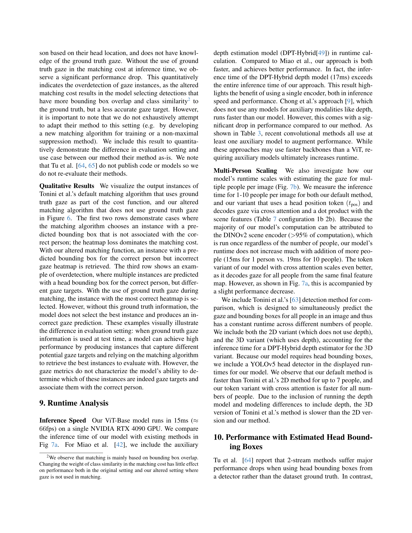
🔼 This table presents the results of an experiment investigating the impact of input image size on gaze estimation performance. Three existing methods (Chong et al., Miao et al., and Gupta et al.) were tested, both in their original forms and with their best-performing variations using a DINOv2 encoder. The input image size was increased from 224x224 to 448x448. The table displays the Area Under the Curve (AUC), average L2 error, and minimum L2 error for each method and image size. The results demonstrate that increasing the input image size does not consistently lead to significant improvements in gaze estimation accuracy, suggesting that a larger input size is not necessary for high performance when high resolution head crops are available.
read the caption
Table 12: Effect of increasing the input scene image size for Chong et al., Miao et al., and Gupta et al.’s original methods and best variants with DINOv2. We do not observe clear gains from using a larger input size.
| Conv Decoder | |
|---|---|
| Conv(d→768, k=1, s=1) | |
| Conv(768→384, k=1, s=1) | |
| Conv(384→192, k=2, s=2) | |
| ConvT(192→96, k=2, s=2) | |
| ConvT(96→1, k=2, s=2) | |
| Conv(1→1, k=1, s=1) | |
| Sigmoid |
🔼 This table details the architectures of two different decoder modules used in the Gaze-LLE model for experiments within Section 3.1. One decoder uses a transformer-based approach, while the other uses a convolutional approach. The table specifies the layer types, input and output dimensions, kernel sizes, strides, and activation functions for each layer in both decoder architectures.
read the caption
Table 13: Architecture details for Transformer Decoder and Convolutional Decoder for experiments in Section 3.1
| Method | AUC ↑ | Avg L2 ↓ | Min L2 ↓ |
|---|---|---|---|
| with ground truth gaze matching | |||
| Tu et al. [64] | 0.917 | 0.133 | 0.069 |
| Tu et al. [65] | 0.928 | 0.114 | 0.057 |
| Tonini et al. [63] | 0.922 | 0.069 | 0.029 |
| Tonini et al.* [63] | 0.924 | 0.068 | 0.030 |
| no ground truth gaze matching | |||
| Tonini et al.* [63] | 0.767 | 0.211 | 0.148 |
| Ours | 0.956 | 0.104 | 0.045 |
🔼 This table compares the performance of Gaze-LLE with detection-based methods (Tu et al. [64, 65], Tonini et al. [63]) on the GazeFollow dataset. The comparison is complicated because the detection-based methods use a different evaluation protocol. Specifically, they use bipartite matching with ground truth gaze at test time to assess performance. This differs from Gaze-LLE and traditional approaches that do not utilize ground truth labels during testing. To facilitate a fair comparison, the table shows results for Tonini et al.’s model using a modified matching cost (Equation 7) that excludes ground truth gaze, making the evaluation more comparable to Gaze-LLE’s. Results using the standard (ground truth gaze-based) evaluation method are also included for context.
read the caption
Table 14: Quantitative comparison with detection-based methods on GazeFollow. The results with ground truth gaze matching use the ground truth gaze labels to perform bipartite matching at test time, and thus are not a direct comparison to our method and prior work. The no ground truth gaze matching results report our method compared to Tonini et al.’s model evaluated with the altered matching cost function in Equation 7, which excludes ground truth gaze information. (∗Results we obtained ourselves by running Tonini et al.’s published code.)
| Method | AUC ↑ | Avg L2 ↓ | Min L2 ↓ |
|---|---|---|---|
| ViT-B + GT | 0.956 | 0.104 | 0.045 |
| ViT-B + YOLO | 0.955 | 0.106 | 0.047 |
| ViT-L + GT | 0.958 | 0.099 | 0.041 |
| ViT-L + YOLO | 0.958 | 0.101 | 0.043 |
🔼 This table presents a comparison of Gaze-LLE’s performance using ground truth head bounding boxes versus head detections from a pre-trained YOLOv5 object detector. It demonstrates the robustness of Gaze-LLE by showing consistent performance regardless of whether ground truth or detected head locations are used as input. The metrics compared are AUC, average L2 distance, and minimum L2 distance, assessing the accuracy of gaze prediction. The results highlight the model’s ability to generalize well to real-world scenarios where perfect head bounding box annotations might not be available.
read the caption
Table 15: Gaze-LLE achieves consistent results when using head detections from an out-of-the-box YOLOv5 detector instead of head ground truth bounding boxes.
| Experiment | GazeFollow | VideoAttentionTarget | ||||
|---|---|---|---|---|---|---|
| AUC ↑ | Avg L2 ↓ | Min L2 ↓ | AUC ↑ | L2 ↓ | APin/out ↑ | |
| Frozen Aux. Angle | 0.869 | 0.217 | 0.146 | 0.802 | 0.234 | 0.720 |
| Trained Aux. Angle | 0.896 | 0.196 | 0.127 | 0.832 | 0.199 | 0.800 |
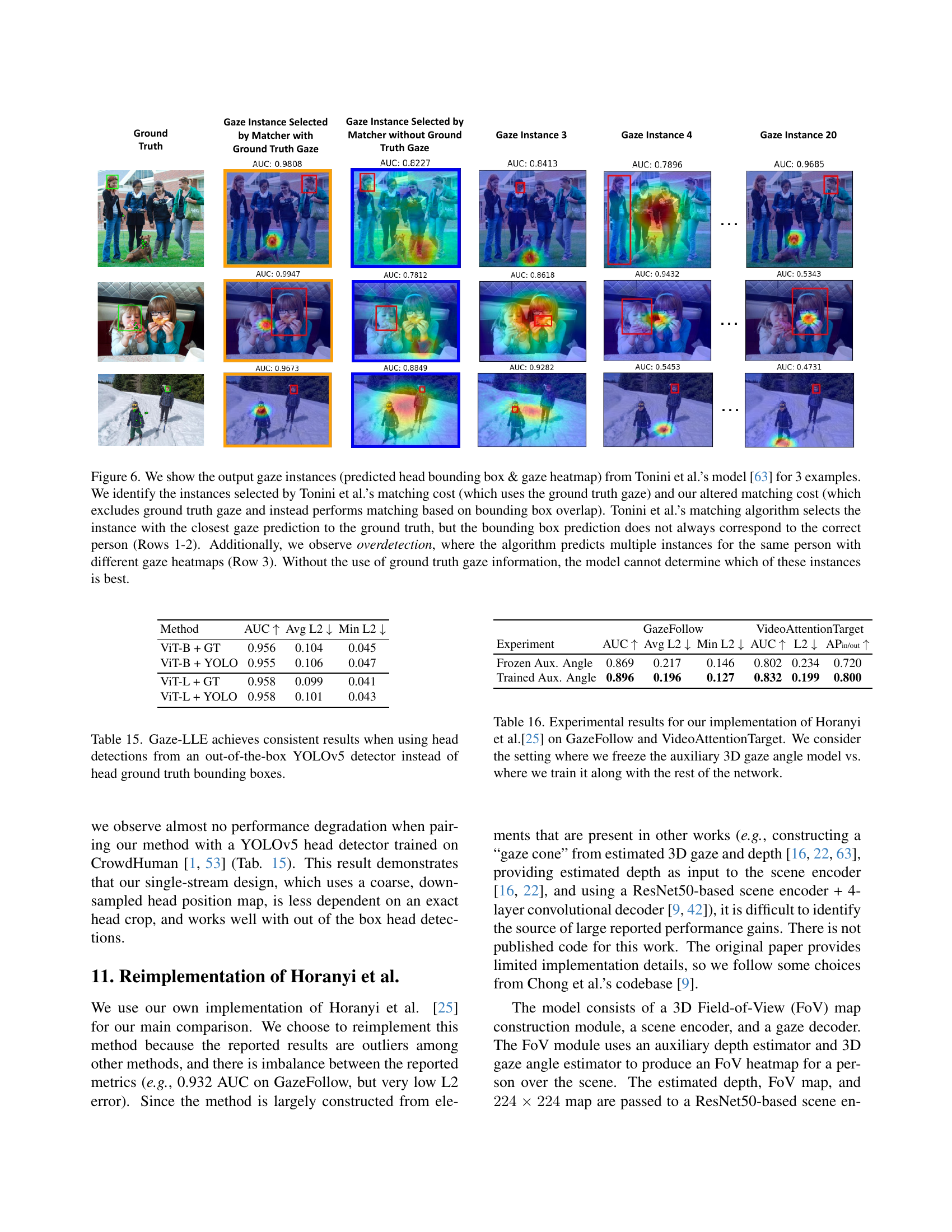
🔼 This table presents a comparison of the performance of a reimplementation of the Horanyi et al. gaze estimation model on two datasets, GazeFollow and VideoAttentionTarget. The model includes auxiliary components for estimating 3D gaze angles and depth. The table shows results under two conditions: one where the auxiliary model’s parameters are frozen during training, and one where it is trained alongside the main model. The comparison highlights how training the auxiliary model affects the overall accuracy (AUC), average L2 error, and minimum L2 error in predicting gaze targets, and also the Average Precision for ‘in/out’ classification (applicable only to VideoAttentionTarget).
read the caption
Table 16: Experimental results for our implementation of Horanyi et al.[25] on GazeFollow and VideoAttentionTarget. We consider the setting where we freeze the auxiliary 3D gaze angle model vs. where we train it along with the rest of the network.
| d_model | Params | AUC ↑ | Avg L2 ↓ | Min L2 ↓ |
|---|---|---|---|---|
| 128 | 1.2M | 0.956 | 0.106 | 0.046 |
| 256 (default) | 2.8M | 0.956 | 0.104 | 0.045 |
| 384 | 5.0M | 0.956 | 0.105 | 0.046 |
| 512 | 7.7M | 0.953 | 0.108 | 0.049 |
| 768 | 14.8M | 0.953 | 0.108 | 0.049 |
🔼 This table presents ablation studies on the dimension of the gaze estimation module within the Gaze-LLE architecture. It shows how varying the dimension (dmodel) of the module, from 128 to 768, affects the model’s performance. The evaluation metrics used are AUC, Avg L2, and Min L2, allowing for a comprehensive assessment of the impact of dmodel on accuracy and localization precision of gaze estimation. The number of parameters in the module are also provided for each dimension.
read the caption
(a) Dimension of gaze estimation module.
| Layers | Params | AUC ↑ | Avg L2 ↓ | Min L2 ↓ |
|---|---|---|---|---|
| 1 layer | 1.2M | 0.953 | 0.115 | 0.054 |
| 2 layers | 2.0M | 0.955 | 0.108 | 0.049 |
| 3 layers | 2.8M | 0.956 | 0.104 | 0.045 |
| 4 layers | 3.6M | 0.956 | 0.103 | 0.045 |
| 5 layers | 4.4M | 0.956 | 0.104 | 0.045 |
🔼 This table presents the ablation study on the number of transformer layers used in the gaze decoder. It shows how the performance (AUC, Avg L2, Min L2) changes as the number of layers increases from 1 to 5, while keeping other hyperparameters constant. The results demonstrate the impact of the number of transformer layers on the model’s accuracy and the trade-off between model complexity and performance.
read the caption
(b) Number of transformer layers.
| Backbone | Params | AUC ↑ | Avg L2 ↓ | Min L2 ↓ |
|---|---|---|---|---|
| One Human | 0.924 | 0.096 | 0.040 | |
| ViT-B | 2.8M | 0.956 | 0.104 | 0.045 |
| ViT-B + LoRA | 3.1M | 0.957 | 0.103 | 0.045 |
| ViT-L | 2.9M | 0.958 | 0.099 | 0.041 |
| ViT-L + LoRA | 3.7M | 0.960 | 0.097 | 0.040 |
🔼 This table presents an ablation study on the architecture of the Gaze-LLE model’s gaze estimation module. Specifically, it examines the impact of varying the internal dimension (dmodel) and the number of transformer layers on the model’s performance. The study uses a ViT-Base DINOv2 backbone and evaluates the results on the GazeFollow dataset. The results show that increasing either the dimension or the number of layers yields diminishing returns in performance after a certain point. Based on this analysis, the researchers selected a dmodel of 256 and 3 transformer layers as the optimal configuration for their default model.
read the caption
Table 17: We investigate the effect of different internal model dimensions and number of transformer layers for our gaze estimation module with a ViT-Base DINOv2 backbone. We observe diminishing returns as we increase the dimension and number of layers. We select dmodel=256subscript𝑑model256d_{\text{model}}=256italic_d start_POSTSUBSCRIPT model end_POSTSUBSCRIPT = 256 with 3 transformer layers as our default configuration.
Full paper#
