↗ arXiv ↗ Hugging Face ↗ Papers with Code
TL;DR#
Key Takeaways#
Why does it matter?#
BLT offers a novel approach to LLM architecture, challenging the reliance on tokenization. It demonstrates byte-level models can be competitive with, and even surpass, token-based models in performance and robustness. This opens new avenues for research in more efficient and adaptable LLMs, impacting how we build and scale these models. BLT’s dynamic compute allocation could reduce the computational costs associated with training and deploying ever-larger LLMs. Its robustness to noise has significant implications for real-world applications. The patching mechanism introduced in BLT could inspire new compression techniques and sequence modeling.
Visual Insights#

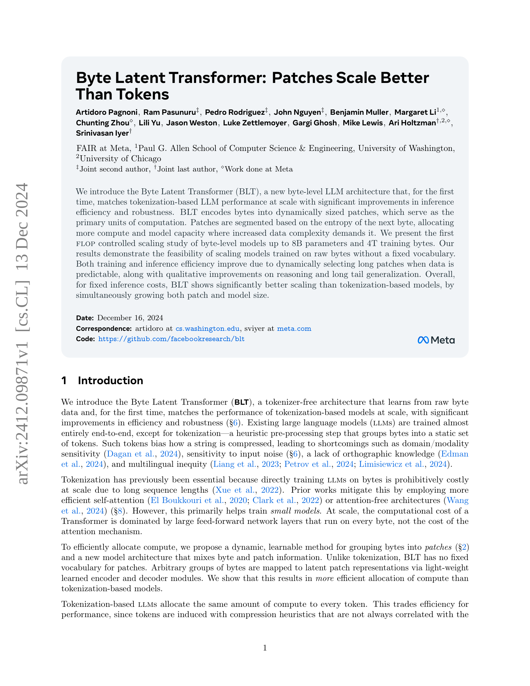
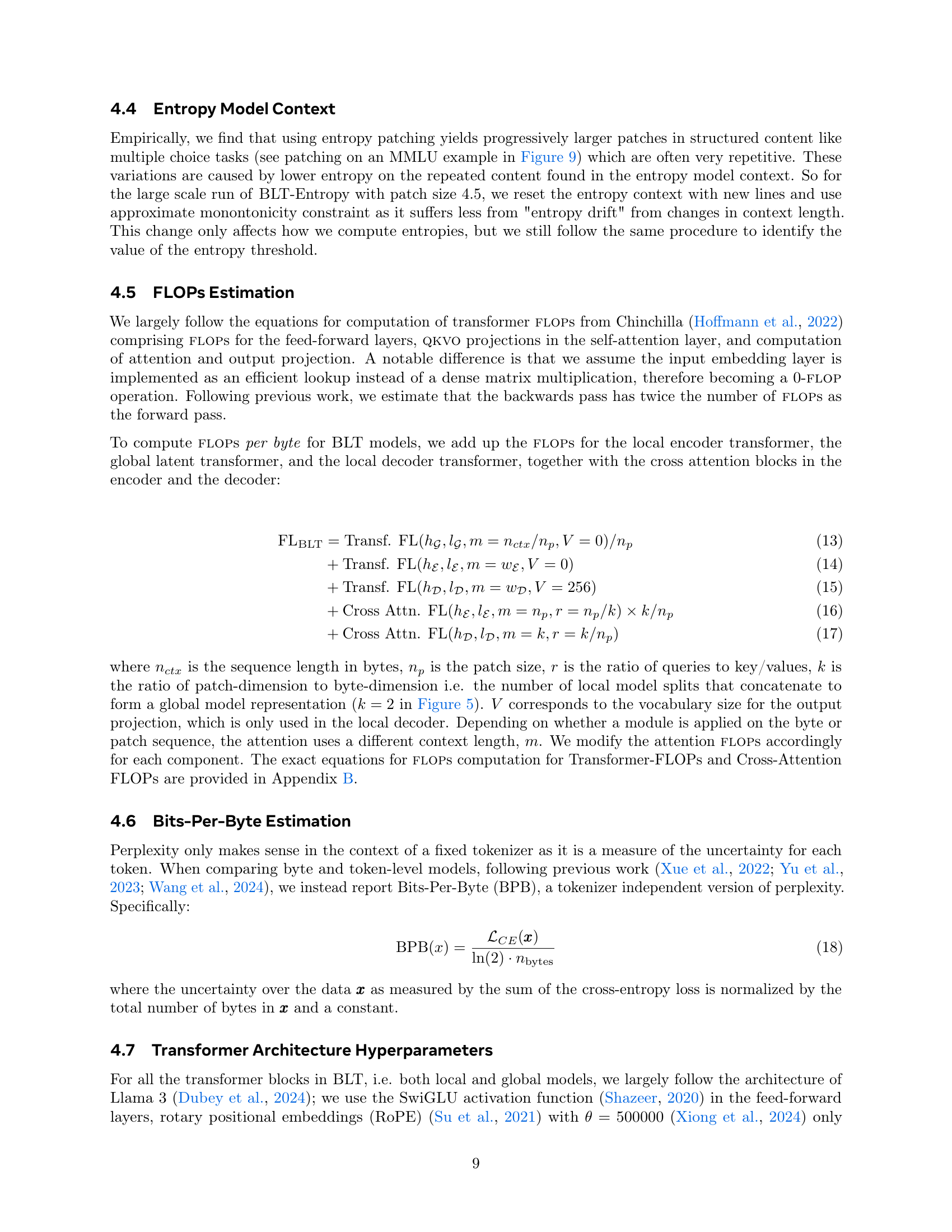
🔼 This figure presents scaling trends of byte-level language models compared to token-based models. It demonstrates that for a fixed inference FLOP budget, BLT models with patch sizes 6 and 8 outperform BPE Llama 2 and 3 models when trained on varying training data sizes. The x-axis represents the training FLOPs, and the y-axis represents the bits-per-byte (BPB). The lower the BPB, the better the performance of the model. As the training data size increases, BLT models achieve lower BPB than the other models. The vertical lines indicate the compute-optimal point for BPE and the crossover point where BLT starts outperforming BPE. The figure highlights that the BLT architecture enables scaling both model and patch size simultaneously for a fixed inference budget, unlike token-based models where the inference budget fixes the model size. The graph also indicates that larger patch sizes (e.g., 8) become more advantageous with larger inference budgets.
read the caption
Figure 1: Scaling trends for fixed inference flop models (fully) trained with varying training budgets. In token-based models, a fixed inference budget determines the model size. In contrast, the BLT architecture provides a new scaling axis allowing simultaneous increases in model and patch size while keeping the same training and inference budget. BLT patch-size (ps) 6 and 8 models quickly overtake scaling trends of bpe Llama 2 and 3. Moving to the larger inference budget makes the larger patch size 8 model more desirable sooner. Both BPE compute-optimal point and crossover point are indicated with vertical lines.
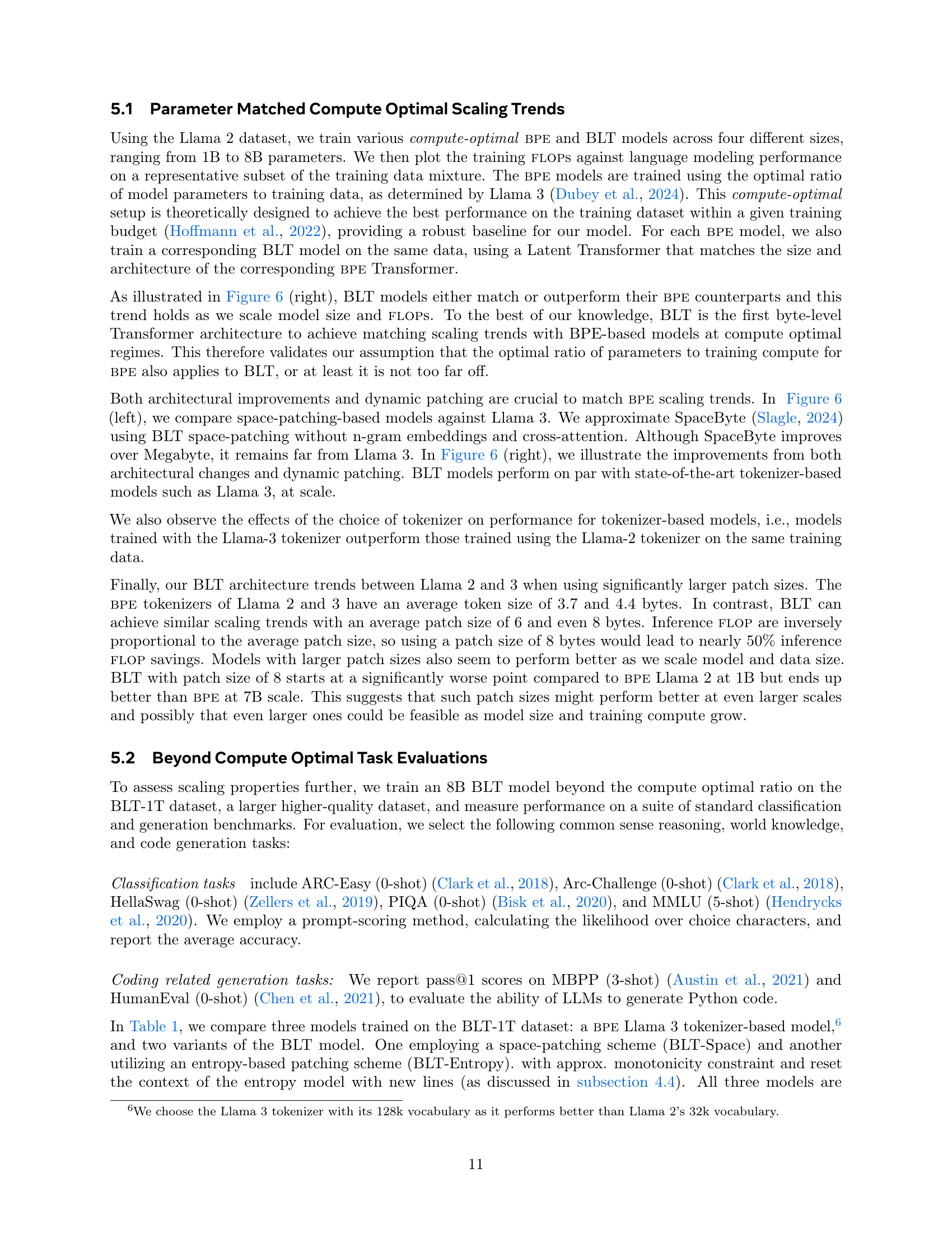
| Llama 3 (1T Tokens) | BLT-Space (6T Bytes) | BLT-Entropy (4.5T Bytes) | |
|---|---|---|---|
| Arc-E | 77.6 | 75.4 | 79.6 |
| Arc-C | 53.3 | 49.8 | 52.1 |
| HellaSwag | 79.1 | 79.6 | 80.6 |
| PIQA | 80.7 | 81.1 | 80.6 |
| MMLU | 58.1 | 54.8 | 57.4 |
| MBPP | 40.2 | 37.6 | 41.8 |
| HumanEval | 31.1 | 27.4 | 35.4 |
| Average | 60.0 | 58.0 | 61.1 |
| Bytes/Patch on Train Mix | 4.4 | 6.1 | 4.5 |
🔼 This table compares the performance of different 8B parameter language models on various benchmarks. The models include a baseline Llama 3 model using the standard Llama 3 tokenizer, and two BLT models trained on the same number of bytes but with different patching schemes: BLT-Space (space patching) and BLT-Entropy (entropy patching). The benchmarks measure zero-shot and few-shot performance on tasks involving common sense reasoning, world knowledge, and code generation. The table shows that BLT models can achieve better average performance than the baseline Llama 3 model while also potentially using significantly fewer FLOPS during inference.
read the caption
Table 1: Comparison of flop-matched BLT 8B models trained on the BLT-1T dataset comprising high-quality tokens of text and code from publicly available sources, with baseline models using the Llama 3 tokenizer. BLT performs better than Llama 3 on average, and depending on the patching scheme, achieves significant flops savings with a minor reduction in performance.
In-depth insights#
Byte-Level LLMs#
Byte-Level LLMs process text as raw bytes, avoiding tokenization. This offers advantages like robustness to noise, handling rare words, and better multilingual support. However, processing long byte sequences presents computational challenges. Some models utilize techniques like dynamic patching to group bytes and efficiently allocate compute resources. This approach has shown promising results, demonstrating competitive performance with token-based models while also offering significant inference cost reductions. Further research focuses on scaling laws and efficient training strategies for byte-level LLMs to unlock their full potential. This also presents advantages in several NLP tasks including machine translation of low resource languages.
Dynamic Patching#
Dynamic patching, as explored in the BLT architecture, revolutionizes compute allocation in LLMs. By dynamically grouping bytes into variable-length patches based on next-byte entropy, BLT focuses compute resources on complex segments, enhancing efficiency and performance. This contrasts sharply with fixed-length patching and tokenization, which allocate compute uniformly regardless of content complexity. BLT’s approach leads to improved inference efficiency, allowing for larger model sizes within the same compute budget. The entropy-based segmentation, using a small byte-level LM to predict next-byte probabilities and define patch boundaries, dynamically adjusts compute allocation based on information density, showing substantial performance improvements over static methods.
BLT Architecture#
The BLT architecture fundamentally rethinks sequence processing by using dynamically sized patches instead of fixed tokens. A small byte-level local encoder first transforms byte sequences into these patches. Then, a larger, more computationally intensive latent transformer processes the patch representations. Finally, another small byte-level decoder converts the processed patches back to bytes. This dynamic patching allows compute allocation based on data complexity, concentrating resources on less predictable areas, improving efficiency, and facilitating the processing of longer sequences. This approach also enhances robustness to noise and understanding of sub-word aspects, addressing common limitations of token-based LLMs.
Scaling & Robustness#
BLT’s dynamic patching allocates compute based on complexity, enabling efficient scaling. Unlike fixed tokenization, BLT adjusts patch size, optimizing for both model size and inference speed. This allows simultaneous scaling, unlike token-based models where a fixed inference budget dictates size. Experiments show BLT matching Llama 3 training performance with up to 50% fewer inference FLOPS. Notably, larger patch sizes in BLT show better scaling trends, suggesting potential for even greater efficiency at larger scales. This flexible scaling, coupled with robustness to input noise and awareness of sub-word units, positions BLT as a promising alternative to traditional methods.
Tokenizer-Free Future#
A tokenizer-free future for Large Language Models (LLMs) offers compelling advantages. Tokenization, a pre-processing step that segments text into discrete units, introduces limitations like vocabulary size constraints and sensitivity to noise. Eliminating this step could enhance model robustness, enabling better handling of noisy or unusual inputs, crucial for real-world applications. Furthermore, a byte-level approach allows the model to learn directly from raw data, potentially uncovering deeper character-level understanding and improving performance on tasks like phonetic transcription or orthographic analysis. By removing the fixed vocabulary, models could also gain adaptability to new data and languages, reducing the need for extensive retraining. This shift also promises improvements in training and inference efficiency by dynamically allocating compute resources based on data complexity. However, a tokenizer-free approach presents challenges such as efficiently handling long sequences and developing effective byte-level training strategies. Despite these hurdles, the potential benefits warrant further exploration into this promising direction for LLM development.
More visual insights#
More on figures

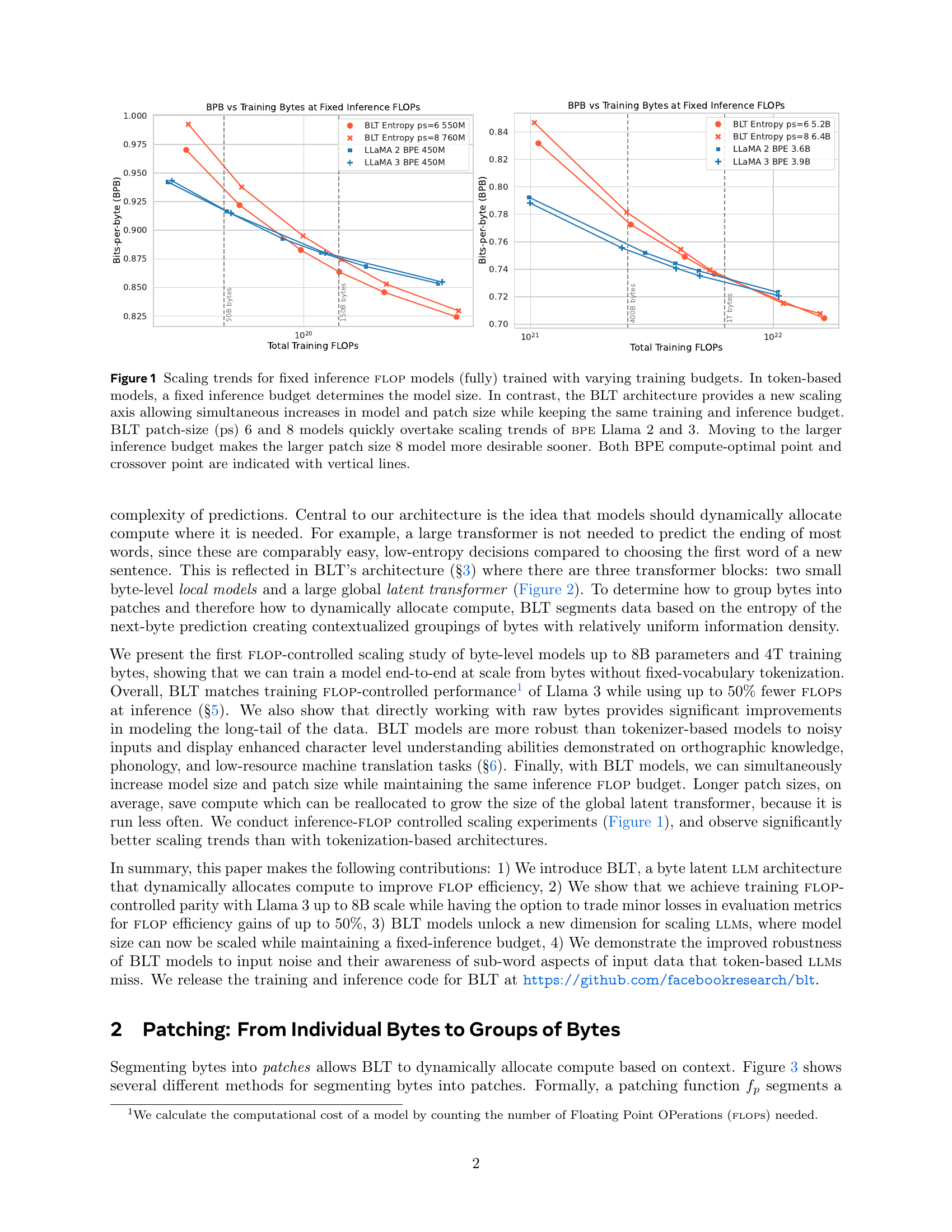
🔼 The figure shows the architecture of the Byte Latent Transformer (BLT). It consists of three main modules: 1) a Local Encoder: This module takes raw bytes as input and encodes them into patch representations. It incorporates byte n-gram embeddings and cross-attention to enhance information flow. 2) a Latent Transformer: This is the core of the model and operates on the patch representations. It’s computationally expensive and serves as a global context processor. 3) a Local Decoder: This lightweight module decodes the patch representations from the Latent Transformer and produces raw byte predictions. Unlike conventional tokenization-based models, BLT maintains direct access to byte-level details by dynamically grouping bytes into patches.
read the caption
Figure 2: BLT comprises three modules, a lightweight Local Encoder that encodes input bytes into patch representations, a computationally expensive Latent Transformer over patch representations, and a lightweight Local Decoder to decode the next patch of bytes. BLT incorporates byte n𝑛nitalic_n-gram embeddings and a cross-attention mechanism to maximize information flow between the Latent Transformer and the byte-level modules (Figure 5). Unlike fixed-vocabulary tokenization, BLT dynamically groups bytes into patches preserving access to the byte-level information.

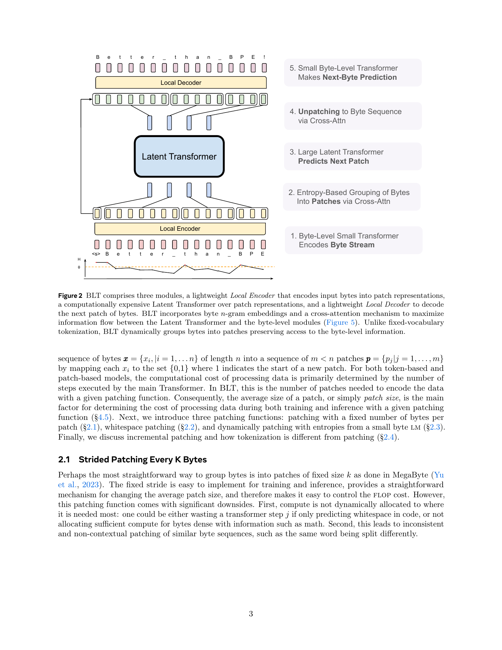
🔼 Figure 3 illustrates various methods for grouping bytes into patches, impacting computational cost. Each patch corresponds to a large transformer step, directly influencing FLOPS expenditure. Methods include: (a) 4-strided patching (MegaByte), (b) BPE tokenization (Llama-3 tokenizer), (c & d) entropy-based patching (this work), (e) space-byte patching, and (f) entropy patching with a CNN byte-level model.
read the caption
Figure 3: Patching schemes group bytes in different ways, each leading to a different number of resulting patches. Since each patch is processed using a large transformer step, the number of patches directly determines the bulk of the compute expended in terms of flops. These schemes group bytes into patches by (a) striding every four bytes (§2.1) as in MegaByte (Yu et al., 2023), (b) tokenizing with Byte-Pair Encoding (bpe), in this case the Llama-3 (Dubey et al., 2024) tokenizer, (c & d) entropy-based patching as in this work (§2.3), (e) patching on space-bytes (Slagle, 2024), (f) and patching on entropy using a small CNN byte-level model with 2-byte context.

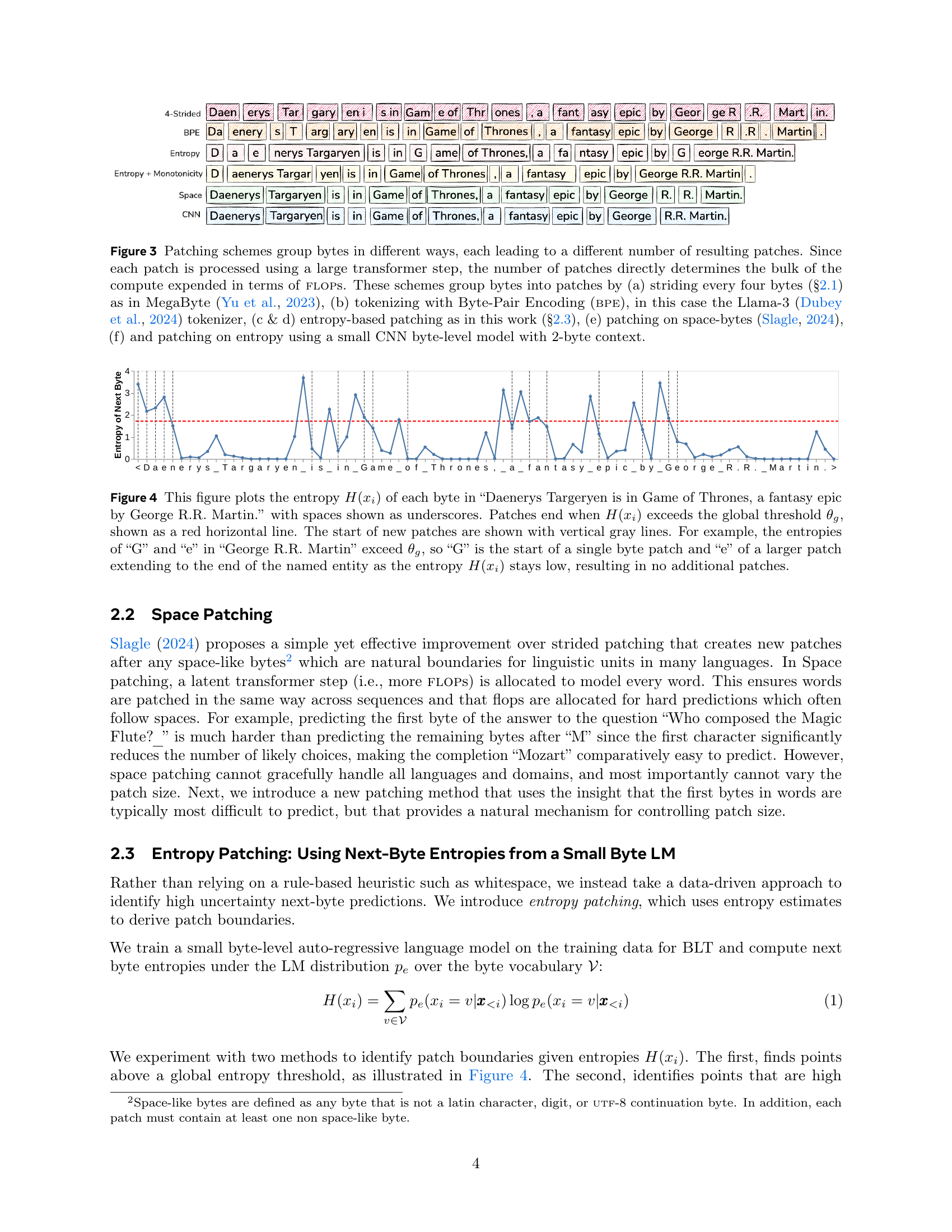
🔼 The figure shows the entropy of each byte in the given example text (‘Daenerys Targaryen is in Game of Thrones, a fantasy epic by George R.R. Martin.’). The x-axis represents each byte and the y-axis entropy. A red horizontal line shows the global threshold. When the entropy of a byte exceeds this threshold, a new patch is started, marked by a vertical gray line. Longer patches occur when the entropy stays low after the first byte. For example, ‘George R.R. Martin’ is split into multiple patches since both ‘G’ and ’e’ have entropy above the threshold, but the next few bytes stay low and extend the ’e’ patch.
read the caption
Figure 4: This figure plots the entropy H(xi)𝐻subscript𝑥𝑖H(x_{i})italic_H ( italic_x start_POSTSUBSCRIPT italic_i end_POSTSUBSCRIPT ) of each byte in “Daenerys Targeryen is in Game of Thrones, a fantasy epic by George R.R. Martin.” with spaces shown as underscores. Patches end when H(xi)𝐻subscript𝑥𝑖H(x_{i})italic_H ( italic_x start_POSTSUBSCRIPT italic_i end_POSTSUBSCRIPT ) exceeds the global threshold θgsubscript𝜃𝑔\theta_{g}italic_θ start_POSTSUBSCRIPT italic_g end_POSTSUBSCRIPT, shown as a red horizontal line. The start of new patches are shown with vertical gray lines. For example, the entropies of “G” and “e” in “George R.R. Martin” exceed θgsubscript𝜃𝑔\theta_{g}italic_θ start_POSTSUBSCRIPT italic_g end_POSTSUBSCRIPT, so “G” is the start of a single byte patch and “e” of a larger patch extending to the end of the named entity as the entropy H(xi)𝐻subscript𝑥𝑖H(x_{i})italic_H ( italic_x start_POSTSUBSCRIPT italic_i end_POSTSUBSCRIPT ) stays low, resulting in no additional patches.

🔼 The local encoder uses a cross-attention mechanism with patch representations as queries and byte representations as keys and values to transform byte representations into patch representations. Similarly, the local decoder uses a cross-attention block but reverses the roles: byte representations serve as queries while patch representations are used as keys and values. The local encoder and decoder enable the model to transition between byte-level and patch-level representations, enhancing the model’s ability to handle both granular byte-level information and higher-level patch-level abstractions. This dual-level processing empowers the model to capture intricate byte-level details while efficiently processing larger chunks of text via patches. In this figure, a Cross-Attn parameter k = 2 is used.
read the caption
Figure 5: The local encoder uses a cross-attention block with patch representations as queries, and byte representations as keys/values to encode byte representations into patch representations. The local decoder uses a similar block but with the roles reversed i.e. byte representations are now the queries and patch representations are the keys/values. Here we use Cross-Attn k=2𝑘2k=2italic_k = 2.

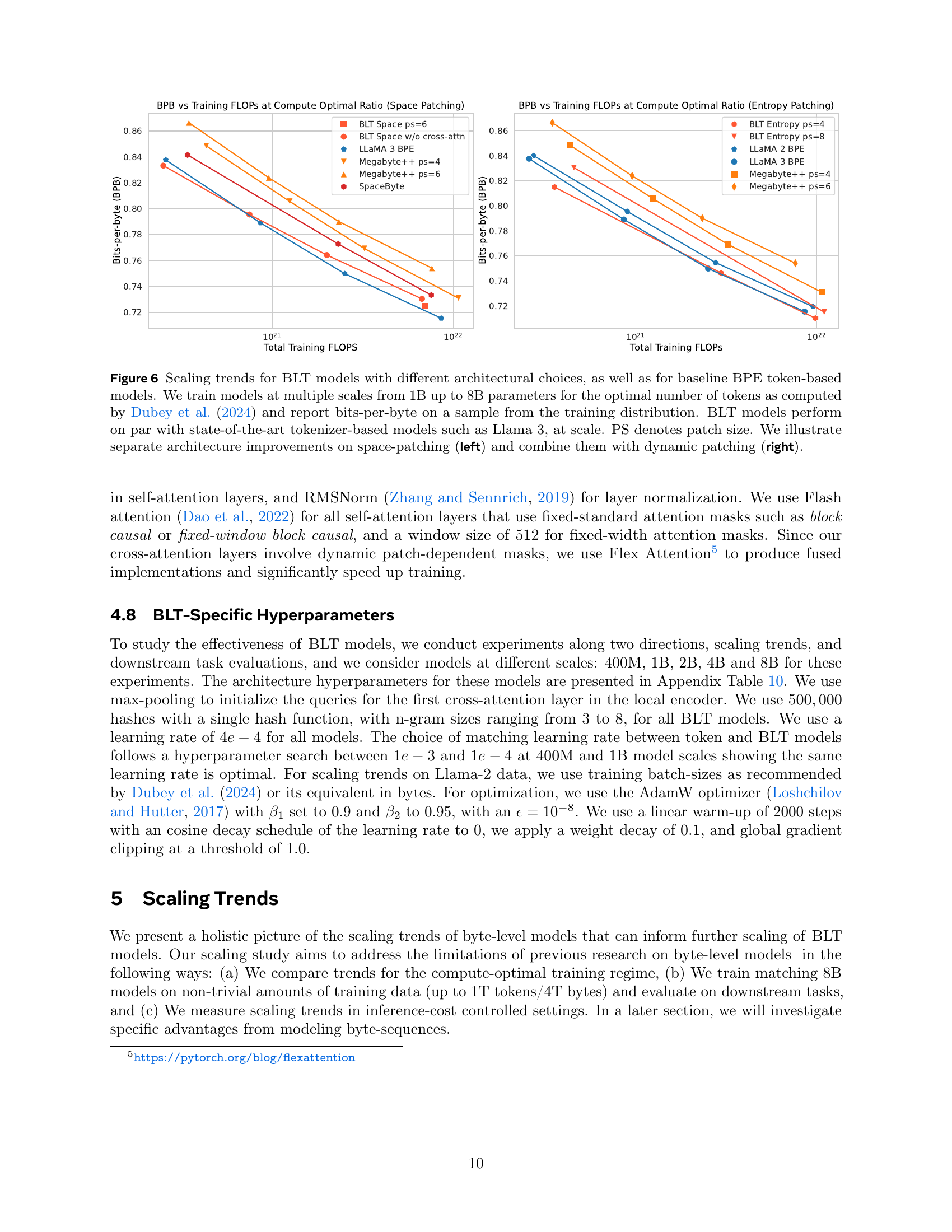
🔼 This figure compares the scaling trends between BLT models with various architectural choices, baseline BPE token-based models (like LLama 2 and 3), and other byte-level models, by plotting training FLOPS against language modeling performance (bits-per-byte). The key takeaway is that BLT models perform comparably to state-of-the-art tokenizer-based models at scale, demonstrating the viability of byte-level models. The left subplot focuses on space-patching and shows architectural improvements. The right subplot demonstrates the improvements achieved by combining architectural changes with dynamic patching.
read the caption
Figure 6: Scaling trends for BLT models with different architectural choices, as well as for baseline BPE token-based models. We train models at multiple scales from 1B up to 8B parameters for the optimal number of tokens as computed by Dubey et al. (2024) and report bits-per-byte on a sample from the training distribution. BLT models perform on par with state-of-the-art tokenizer-based models such as Llama 3, at scale. PS denotes patch size. We illustrate separate architecture improvements on space-patching (left) and combine them with dynamic patching (right).

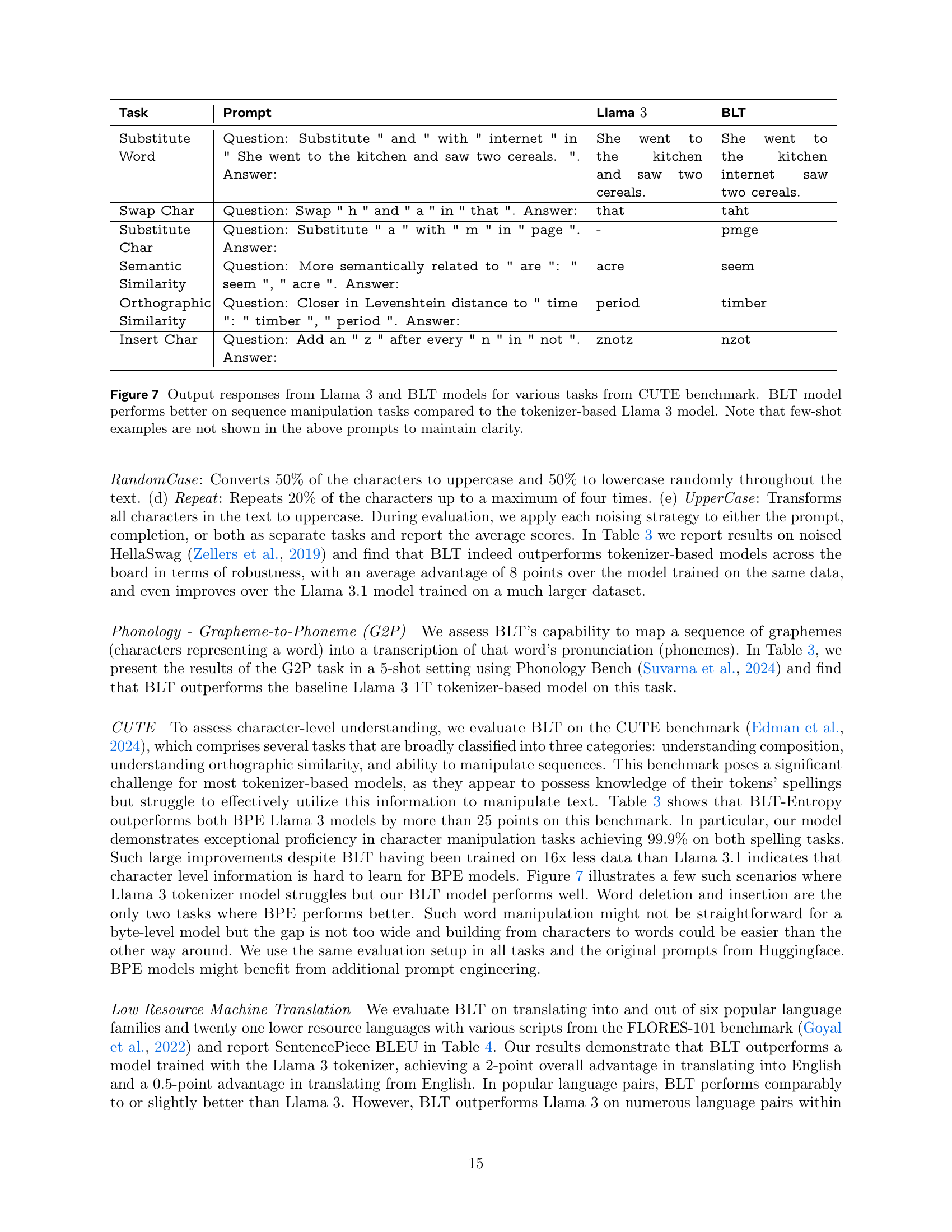
🔼 Figure 7 showcases a comparison between the responses generated by Llama 3 and BLT models on various tasks from the CUTE benchmark. These tasks evaluate character-level understanding and manipulation abilities, including substitution, swapping, semantic similarity, orthographic similarity, and insertion of characters. The prompts used for each task are shown in the figure, but few-shot examples are omitted for clarity. The results highlight BLT’s superior performance on sequence manipulation tasks, indicating a better understanding and ability to manipulate text at the character level compared to the token-based Llama 3.
read the caption
Figure 7: Output responses from Llama 3 and BLT models for various tasks from CUTE benchmark. BLT model performs better on sequence manipulation tasks compared to the tokenizer-based Llama 3 model. Note that few-shot examples are not shown in the above prompts to maintain clarity.

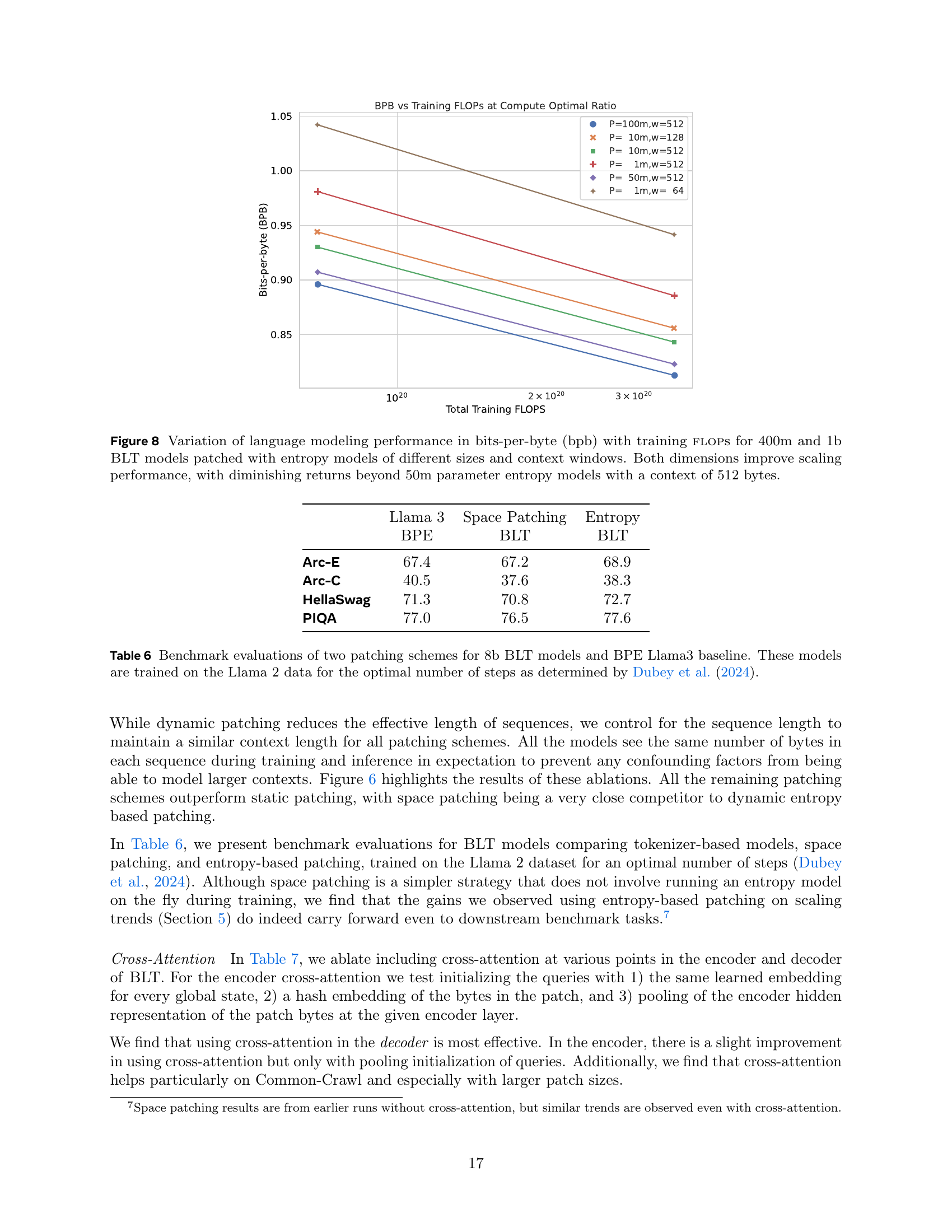
🔼 This figure analyzes the impact of entropy model size and context window length on the performance of 400 million and 1 billion parameter BLT models. The x-axis represents training FLOPS, and the y-axis represents bits-per-byte (bpb), a measure of language modeling performance. Different lines correspond to varying entropy model sizes (1m, 10m, 50m, and 100m parameters) and context window lengths (64, 128, and 512 bytes). The results indicate that increasing both entropy model size and context window length improves performance, but with diminishing returns beyond 50 million parameter entropy models with a 512-byte context window.
read the caption
Figure 8: Variation of language modeling performance in bits-per-byte (bpb) with training flops for 400m and 1b BLT models patched with entropy models of different sizes and context windows. Both dimensions improve scaling performance, with diminishing returns beyond 50m parameter entropy models with a context of 512 bytes.
More on tables
| Llama 3 |
|---|
| 1T Tokens |
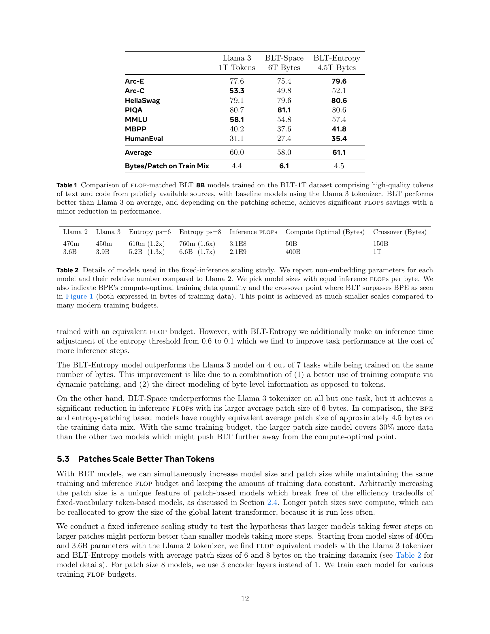
🔼 This table presents details of the models used in the fixed-inference scaling study, comparing BLT (Byte Latent Transformer) models to Llama 2 and Llama 3 models. It includes information about model parameters, training FLOPS (Floating Point Operations), and training data size. Notably, the table highlights the crossover point where BLT models outperform BPE models in terms of performance and the amount of training data required for this to happen. The table illustrates that the crossover point occurs at a much smaller scale than is typically used in current large language model training, suggesting the efficiency of the BLT approach.
read the caption
Table 2: Details of models used in the fixed-inference scaling study. We report non-embedding parameters for each model and their relative number compared to Llama 2. We pick model sizes with equal inference flops per byte. We also indicate BPE’s compute-optimal training data quantity and the crossover point where BLT surpasses BPE as seen in Figure 1 (both expressed in bytes of training data). This point is achieved at much smaller scales compared to many modern training budgets.
| BLT-Space |
|---|
| 6T Bytes |
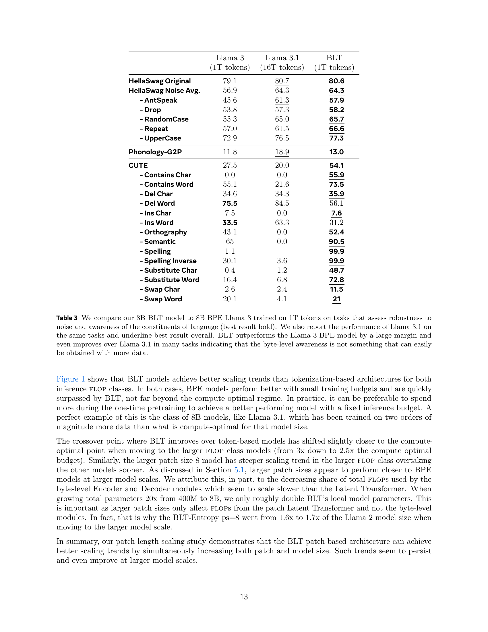
🔼 This table presents a comparison of an 8B parameter BLT model with two 8B parameter Llama 3 models on several tasks. One Llama 3 model is trained on 1 trillion tokens while another (Llama 3.1) is trained on 16 trillion tokens. The tasks include the HellaSwag benchmark with several noisy variations where characters are dropped, repeated, substituted, cased differently, or converted to ‘antspeak’ (uppercase characters separated by spaces), the grapheme-to-phoneme task from the Phonology Bench dataset, and the CUTE benchmark with several character manipulation tasks such as character and word insertion/deletion/substitution/swapping, as well as a semantic similarity and orthographic similarity task. The BLT model outperforms the Llama 3 model trained on the same amount of data by a large margin and even improves over Llama 3.1 trained on much more data in many of the tasks, especially the robustness-to-noise and character manipulation tasks, indicating that the byte-level awareness is hard to learn with BPE-based models even with substantially more training data.
read the caption
Table 3: We compare our 8B BLT model to 8B BPE Llama 3 trained on 1T tokens on tasks that assess robustness to noise and awareness of the constituents of language (best result bold). We also report the performance of Llama 3.1 on the same tasks and underline best result overall. BLT outperforms the Llama 3 BPE model by a large margin and even improves over Llama 3.1 in many tasks indicating that the byte-level awareness is not something that can easily be obtained with more data.
| BLT-Entropy |
|---|
| 4.5T Bytes |
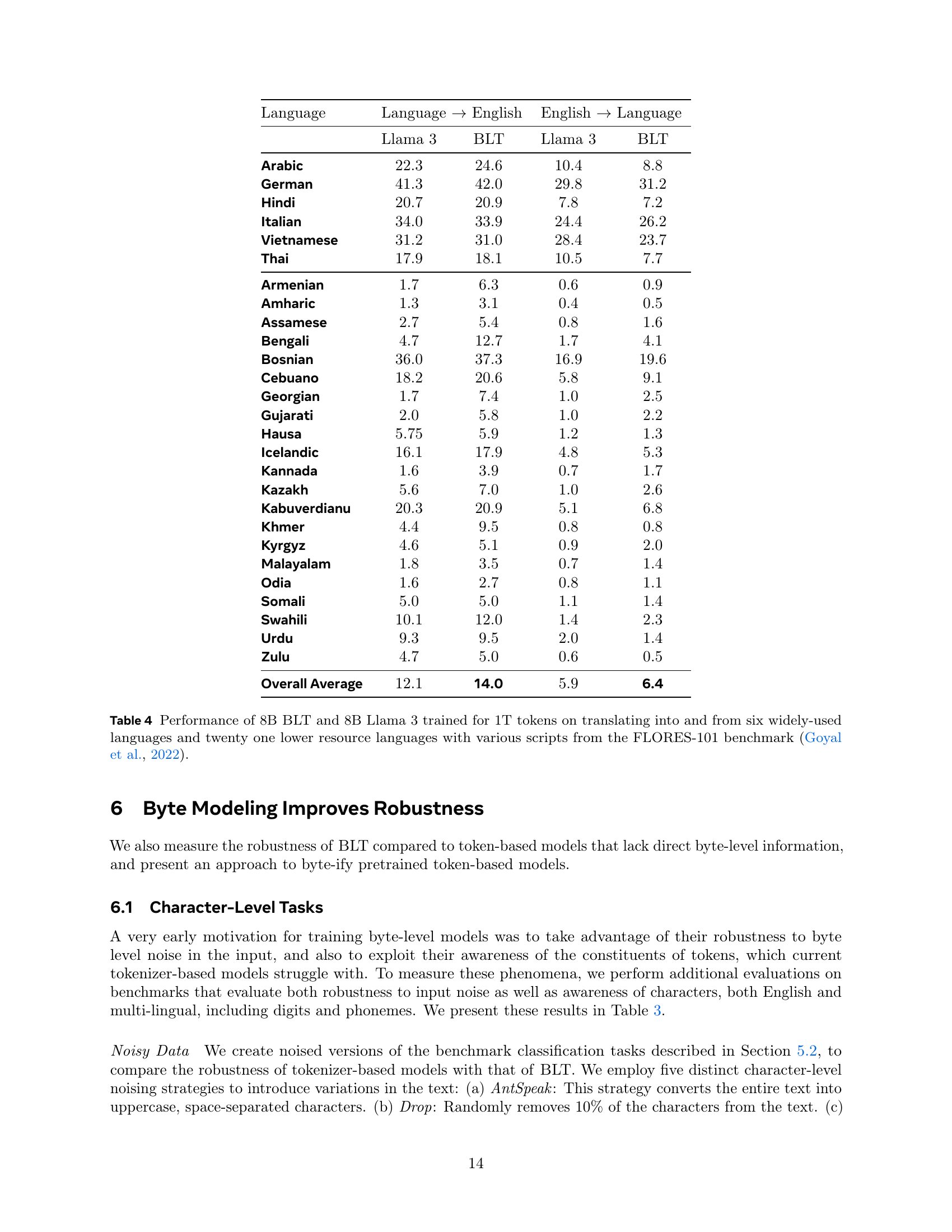
🔼 This table presents the BLEU scores of 8B BLT and 8B Llama 3 models, both trained on 1 trillion tokens, for translation tasks on the FLORES-101 benchmark. FLORES-101 includes 6 high-resource languages and 21 low-resource languages. The results are separated for translation into English and from English. This allows for evaluating the models’ performance on a diverse range of languages and scripts, highlighting byte modeling’s advantages in long-tail generalization.
read the caption
Table 4: Performance of 8B BLT and 8B Llama 3 trained for 1T tokens on translating into and from six widely-used languages and twenty one lower resource languages with various scripts from the FLORES-101 benchmark (Goyal et al., 2022).
| Llama 2 | Llama 3 | Entropy ps=6 | Entropy ps=8 | Inference FLOPs | Compute Optimal (Bytes) | Crossover (Bytes) |
|---|---|---|---|---|---|---|
| 470m | 450m | 610m (1.2x) | 760m (1.6x) | 3.1E8 | 50B | 150B |
| 3.6B | 3.9B | 5.2B (1.3x) | 6.6B (1.7x) | 2.1E9 | 400B | 1T |
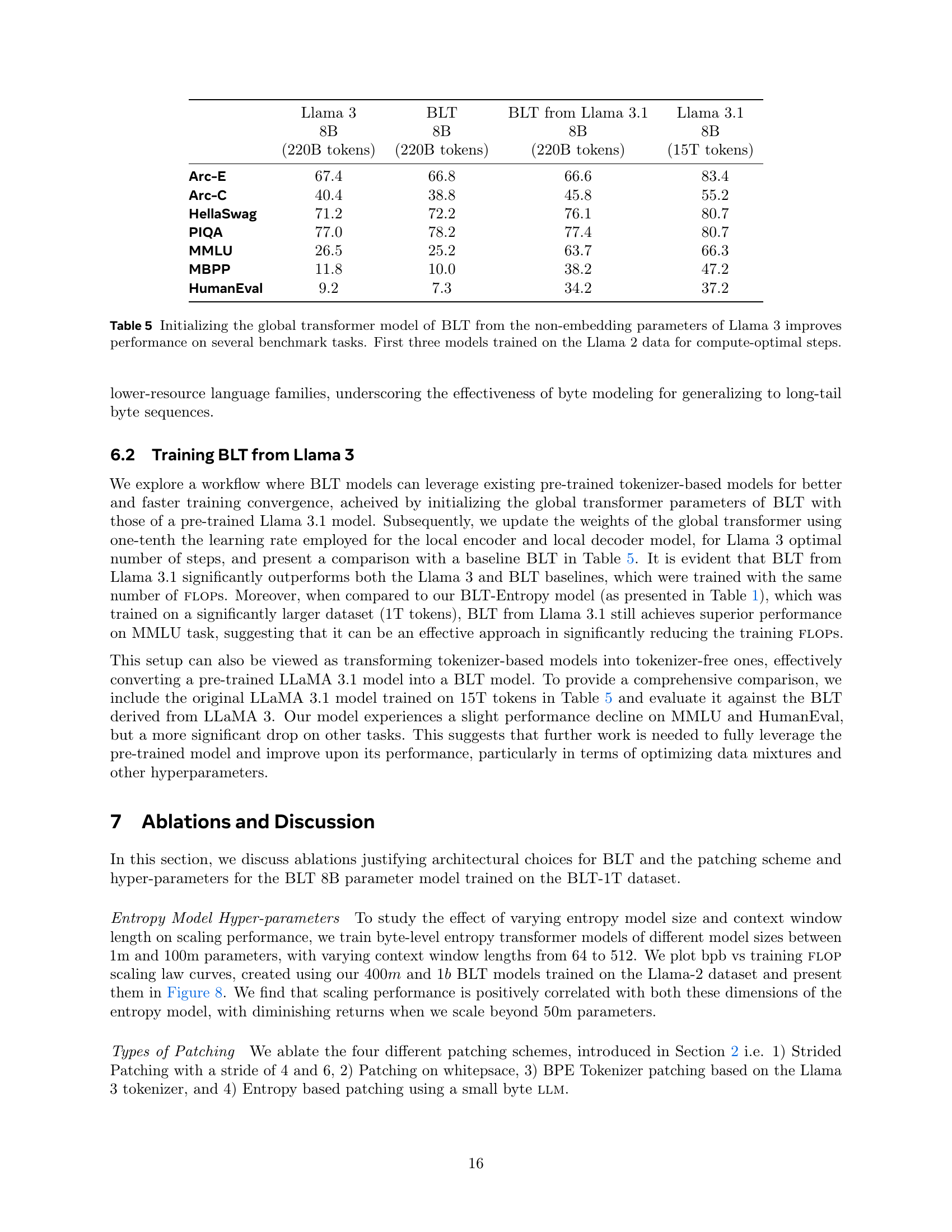
🔼 This table compares the performance of different 8B parameter models on several benchmark tasks. It includes models like LLaMA 3, BLT, and a version of BLT initialized from LLaMA 3 weights. The first three models (LLaMA 3, BLT, BLT initialized from LLaMA 3) are trained on the LLaMA 2 dataset using a compute-optimal training strategy. The last model, LLaMA 3.1, is also included for reference, and it’s trained on a significantly larger dataset (15T tokens) than the other models. The results suggest that initializing BLT from pre-trained LLaMA 3 weights leads to improved performance across different tasks.
read the caption
Table 5: Initializing the global transformer model of BLT from the non-embedding parameters of Llama 3 improves performance on several benchmark tasks. First three models trained on the Llama 2 data for compute-optimal steps.
| Llama 3 (1T tokens) | Llama 3.1 (16T tokens) | BLT (1T tokens) | |
|---|---|---|---|
| HellaSwag Original | 79.1 | 80.7 | 80.6 |
| HellaSwag Noise Avg. | 56.9 | 64.3 | 64.3 |
| - AntSpeak | 45.6 | 61.3 | 57.9 |
| - Drop | 53.8 | 57.3 | 58.2 |
| - RandomCase | 55.3 | 65.0 | 65.7 |
| - Repeat | 57.0 | 61.5 | 66.6 |
| - UpperCase | 72.9 | 76.5 | 77.3 |
| Phonology-G2P | 11.8 | 18.9 | 13.0 |
| CUTE | 27.5 | 20.0 | 54.1 |
| - Contains Char | 0.0 | 0.0 | 55.9 |
| - Contains Word | 55.1 | 21.6 | 73.5 |
| - Del Char | 34.6 | 34.3 | 35.9 |
| - Del Word | 75.5 | 84.5 | 56.1 |
| - Ins Char | 7.5 | 0.0 | 7.6 |
| - Ins Word | 33.5 | 63.3 | 31.2 |
| - Orthography | 43.1 | 0.0 | 52.4 |
| - Semantic | 65 | 0.0 | 90.5 |
| - Spelling | 1.1 | - | 99.9 |
| - Spelling Inverse | 30.1 | 3.6 | 99.9 |
| - Substitute Char | 0.4 | 1.2 | 48.7 |
| - Substitute Word | 16.4 | 6.8 | 72.8 |
| - Swap Char | 2.6 | 2.4 | 11.5 |
| - Swap Word | 20.1 | 4.1 | 21 |
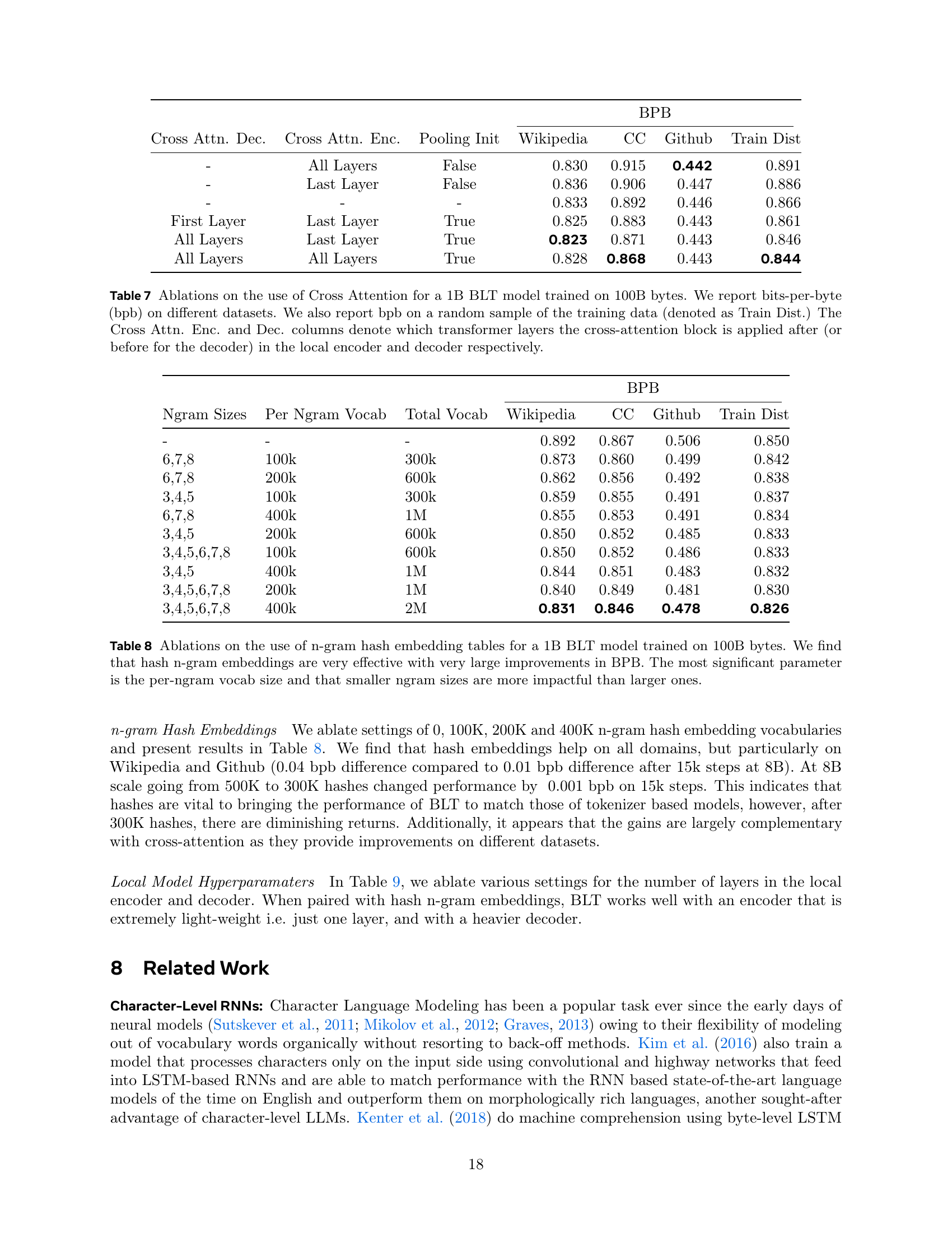
🔼 This table presents benchmark results comparing an 8B parameter BPE Llama 3 tokenizer-based model with two 8B parameter BLT models, one with Space patching and the other with Entropy patching. All models were trained on the Llama 2 dataset for an optimal number of training steps as determined by Dubey et al. (2024). The metrics used for evaluation include ARC-Easy, ARC-Challenge, HellaSwag, and PIQA. The goal is to demonstrate that dynamic entropy-based patching allows the BLT model to achieve similar or better performance compared to the BPE baseline, despite the simpler patching strategy.
read the caption
Table 6: Benchmark evaluations of two patching schemes for 8b BLT models and BPE Llama3 baseline. These models are trained on the Llama 2 data for the optimal number of steps as determined by Dubey et al. (2024).
| Llama 3 |
|---|
| (1T tokens) |
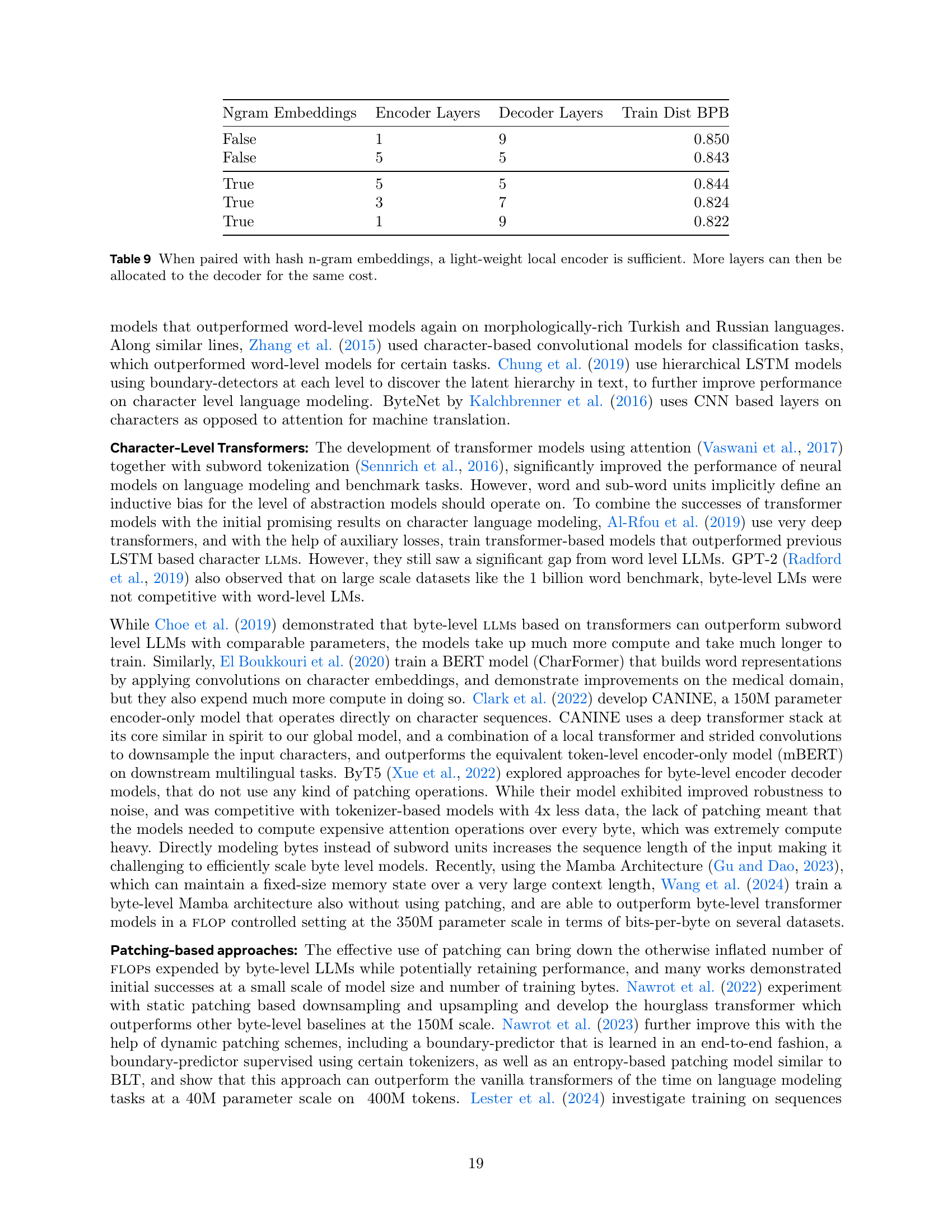
🔼 This table presents an ablation study on the effects of applying a cross-attention mechanism at different layers within the encoder and decoder modules of a 1B parameter Byte Latent Transformer (BLT) model. The model is trained on 100B bytes of text data. The table reports the bits-per-byte (bpb) performance of these models on different datasets, including Wikipedia, Common Crawl (CC), Github, and a random sample from the training data distribution (Train Dist). The table investigates whether applying cross-attention to all layers, the last layer, or the first layer of the encoder and decoder impacts performance. It also includes a ‘Pooling Init’ column which indicates an alternative initialization of the cross-attention queries for the final patch representation.
read the caption
Table 7: Ablations on the use of Cross Attention for a 1B BLT model trained on 100B bytes. We report bits-per-byte (bpb) on different datasets. We also report bpb on a random sample of the training data (denoted as Train Dist.) The Cross Attn. Enc. and Dec. columns denote which transformer layers the cross-attention block is applied after (or before for the decoder) in the local encoder and decoder respectively.
| Llama 3.1 |
|---|
| (16T tokens) |
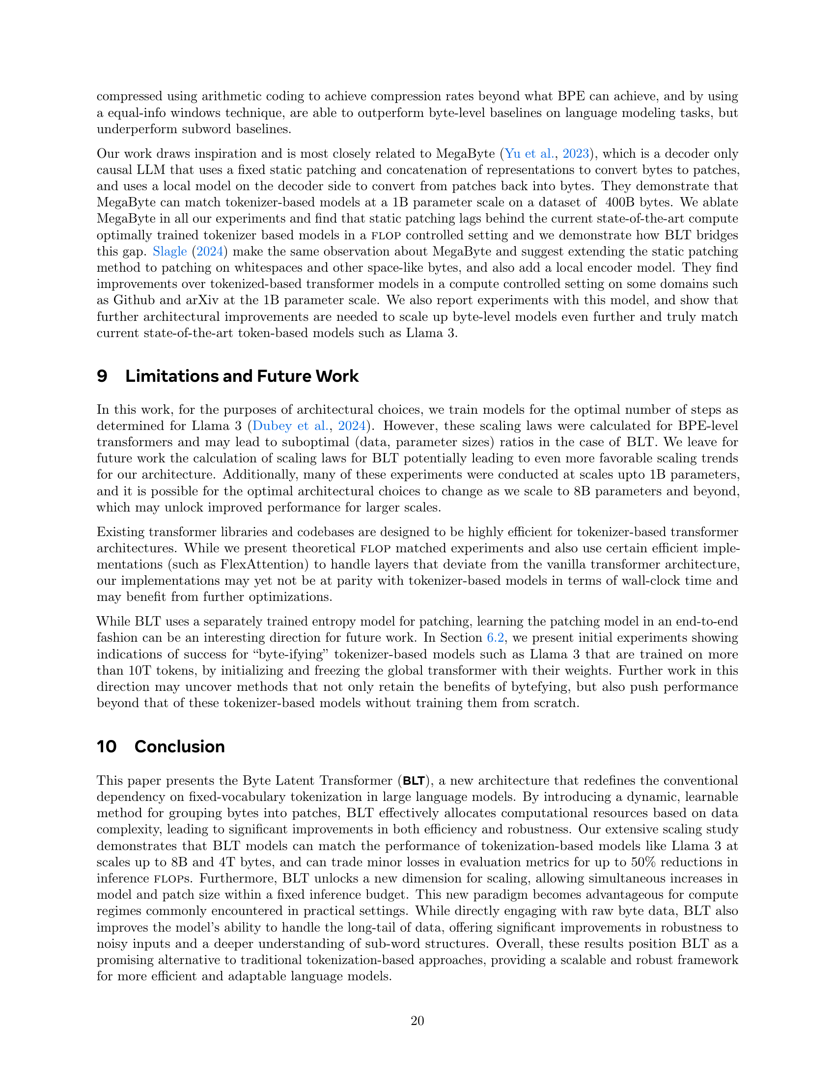
🔼 This table presents an ablation study on the use of n-gram hash embedding tables for a 1B parameter Byte Latent Transformer (BLT) model trained on 100B bytes. The table explores different n-gram sizes (3-8) and per-n-gram vocabulary sizes (50k, 100k, 200k, and 400k), evaluating their impact on bits-per-byte (BPB) across various datasets (Wikipedia, Common Crawl, GitHub, and a training data distribution). The results demonstrate that incorporating hash n-gram embeddings significantly improves language modeling performance by reducing BPB. The study also reveals that the vocabulary size allocated to each n-gram is a critical factor, with larger vocabulary sizes generally leading to better performance. Furthermore, smaller n-gram sizes appear to be more influential than larger ones in enhancing performance.
read the caption
Table 8: Ablations on the use of n-gram hash embedding tables for a 1B BLT model trained on 100B bytes. We find that hash n-gram embeddings are very effective with very large improvements in BPB. The most significant parameter is the per-ngram vocab size and that smaller ngram sizes are more impactful than larger ones.
| BLT |
|---|
| (1T tokens) |
🔼 This table presents an ablation study on the number of encoder and decoder layers in a 1B parameter BLT model trained on 100B bytes. The study investigates the impact of varying the number of layers in the local encoder and decoder modules on the model’s performance, as measured by bits-per-byte (BPB) on a held-out training data set. The table also includes a condition where n-gram embeddings are not used. The results suggest that when hash n-gram embeddings are employed, a lightweight local encoder with fewer layers is sufficient, and more layers can be allocated to the decoder for improved performance without increasing computational cost.
read the caption
Table 9: When paired with hash n-gram embeddings, a light-weight local encoder is sufficient. More layers can then be allocated to the decoder for the same cost.
| Language | Language → English | English → Language | ||
|---|---|---|---|---|
| Llama 3 | BLT | Llama 3 | BLT | |
| Arabic | 22.3 | 24.6 | 10.4 | 8.8 |
| German | 41.3 | 42.0 | 29.8 | 31.2 |
| Hindi | 20.7 | 20.9 | 7.8 | 7.2 |
| Italian | 34.0 | 33.9 | 24.4 | 26.2 |
| Vietnamese | 31.2 | 31.0 | 28.4 | 23.7 |
| Thai | 17.9 | 18.1 | 10.5 | 7.7 |
| Armenian | 1.7 | 6.3 | 0.6 | 0.9 |
| Amharic | 1.3 | 3.1 | 0.4 | 0.5 |
| Assamese | 2.7 | 5.4 | 0.8 | 1.6 |
| Bengali | 4.7 | 12.7 | 1.7 | 4.1 |
| Bosnian | 36.0 | 37.3 | 16.9 | 19.6 |
| Cebuano | 18.2 | 20.6 | 5.8 | 9.1 |
| Georgian | 1.7 | 7.4 | 1.0 | 2.5 |
| Gujarati | 2.0 | 5.8 | 1.0 | 2.2 |
| Hausa | 5.75 | 5.9 | 1.2 | 1.3 |
| Icelandic | 16.1 | 17.9 | 4.8 | 5.3 |
| Kannada | 1.6 | 3.9 | 0.7 | 1.7 |
| Kazakh | 5.6 | 7.0 | 1.0 | 2.6 |
| Kabuverdianu | 20.3 | 20.9 | 5.1 | 6.8 |
| Khmer | 4.4 | 9.5 | 0.8 | 0.8 |
| Kyrgyz | 4.6 | 5.1 | 0.9 | 2.0 |
| Malayalam | 1.8 | 3.5 | 0.7 | 1.4 |
| Odia | 1.6 | 2.7 | 0.8 | 1.1 |
| Somali | 5.0 | 5.0 | 1.1 | 1.4 |
| Swahili | 10.1 | 12.0 | 1.4 | 2.3 |
| Urdu | 9.3 | 9.5 | 2.0 | 1.4 |
| Zulu | 4.7 | 5.0 | 0.6 | 0.5 |
| Overall Average | 12.1 | 14.0 | 5.9 | 6.4 |
🔼 This table lists the architectural hyperparameters used for different Byte Latent Transformer (BLT) model sizes in FLOP-controlled experiments. It includes parameters for the local encoder, global latent transformer, and local decoder modules. Key hyperparameters include the number of layers (l), number of attention heads, hidden dimension (h), number of parameters, and cross-attention parameters (k). This table is used to detail the architecture of different sized BLT models in FLOP-controlled scaling experiments. Different configurations are shown for models with 400M, 1B, 2B, 4B, and 8B parameters. Details for the encoder, global latent transformer, decoder and cross attention modules are broken down for each model size.
read the caption
Table 10: Architectural hyper-parameters for different BLT model sizes that we train for flop-controlled experiments described in this paper.
| Task | Prompt | Llama 3 | BLT |
|---|---|---|---|
| Substitute Word | Question: Substitute " and " with " internet " in " She went to the kitchen and saw two cereals. “. Answer: | She went to the kitchen and saw two cereals. | She went to the kitchen internet saw two cereals. |
| Swap Char | Question: Swap " h " and " a " in " that “. Answer: | that | taht |
| Substitute Char | Question: Substitute " a " with " m " in " page “. Answer: | - | pmge |
| Semantic Similarity | Question: More semantically related to " are “: " seem “, " acre “. Answer: | acre | seem |
| Orthographic Similarity | Question: Closer in Levenshtein distance to " time “: " timber “, " period “. Answer: | period | timber |
| Insert Char | Question: Add an " z " after every " n " in " not “. Answer: | znotz | nzot |
🔼 This table shows FLOPS calculations of basic operations including attention, QKVO, Feed-forward, De-Embedding and Cross-Attention used in transformer and BLT model computations in this paper. The table specifies FLOPS parameters: l (layers), h (hidden dimension), hk (hidden dimension with n_heads), m (context length), dff (feed-forward dimension multiplier where dff=4), p (patch size) and r (ratio of queries to keys). It is assumed that the backward pass uses twice as much FLOPS as the forward pass in FLOPS equations.
read the caption
Table 11: flops for operations used in transformer and BLT models. l𝑙litalic_l corresponds to layers, hℎhitalic_h is the hidden dimension (hksubscriptℎ𝑘h_{k}italic_h start_POSTSUBSCRIPT italic_k end_POSTSUBSCRIPT with nheadssubscript𝑛ℎ𝑒𝑎𝑑𝑠n_{heads}italic_n start_POSTSUBSCRIPT italic_h italic_e italic_a italic_d italic_s end_POSTSUBSCRIPT heads), m𝑚mitalic_m is the context length, dff=4subscript𝑑𝑓𝑓4d_{ff}=4italic_d start_POSTSUBSCRIPT italic_f italic_f end_POSTSUBSCRIPT = 4 is the feed-forward dimension multiplier, p𝑝pitalic_p is the patch size, and r𝑟ritalic_r is the ratio of queries to keys.
| Llama 3 8B (220B tokens) | BLT 8B (220B tokens) | BLT from Llama 3.1 8B (220B tokens) | Llama 3.1 8B (15T tokens) | |
|---|---|---|---|---|
| Arc-E | 67.4 | 66.8 | 66.6 | 83.4 |
| Arc-C | 40.4 | 38.8 | 45.8 | 55.2 |
| HellaSwag | 71.2 | 72.2 | 76.1 | 80.7 |
| PIQA | 77.0 | 78.2 | 77.4 | 80.7 |
| MMLU | 26.5 | 25.2 | 63.7 | 66.3 |
| MBPP | 11.8 | 10.0 | 38.2 | 47.2 |
| HumanEval | 9.2 | 7.3 | 34.2 | 37.2 |
🔼 This table compares the bits-per-byte (BPB) performance and perplexity of different n-gram embedding strategies in a 1 billion parameter Byte Latent Transformer (BLT) model trained on 100 billion bytes of text. It specifically ablates the use of frequency-based and hash-based n-gram embedding tables, varying parameters like n-gram sizes and vocabulary size. The table also reports perplexity across different text domains like Wikipedia, Common Crawl, Github, and the training data distribution to assess the effectiveness of these strategies. This comparison highlights the efficacy of both n-gram types in enhancing language modeling performance but showcases hash n-gram embeddings as generally more beneficial due to its ability to overcome vocabulary limitations. Further analyses demonstrate that smaller n-gram sizes often yield better performance gains.
read the caption
Table 12: Ablations on the use of frequency-based as well as hash-based n-gram embedding tables for a 1B BLT model trained on 100B bytes.
Full paper#
