↗ arXiv ↗ Hugging Face ↗ Papers with Code
TL;DR#
Creating realistic 3D scenes from a single image is challenging, especially when multiple objects are involved. Existing methods, often designed for single objects, struggle with consistent object placement and appearance when applied to complex scenes. This lack of “structural awareness” leads to unrealistic or distorted images under novel viewpoints, hindering progress in applications like AR/VR.
MOVIS enhances the 3D structural awareness by incorporating depth and object masks as additional inputs to the diffusion model, and predicting object masks under target view as an auxiliary task. A structure-guided timestep sampling schedule balances learning global placements and local details. New metrics, including cross-view consistency, are introduced for better evaluation, showcasing improved performance and stronger generalization to unseen datasets. This structured approach improves object placement and appearance consistency in multi-object novel view synthesis.
Key Takeaways#
Why does it matter?#
Enhancing multi-object novel view synthesis is crucial for various applications like AR/VR and robotics. This paper’s focus on structural awareness in diffusion models addresses a significant gap in current research, paving the way for more realistic and consistent 3D scene generation. The proposed evaluation metrics for cross-view consistency also offer valuable tools for future research, enabling a more robust assessment of NVS models in complex environments and opening new avenues for research in 3D scene understanding and generation.
Visual Insights#

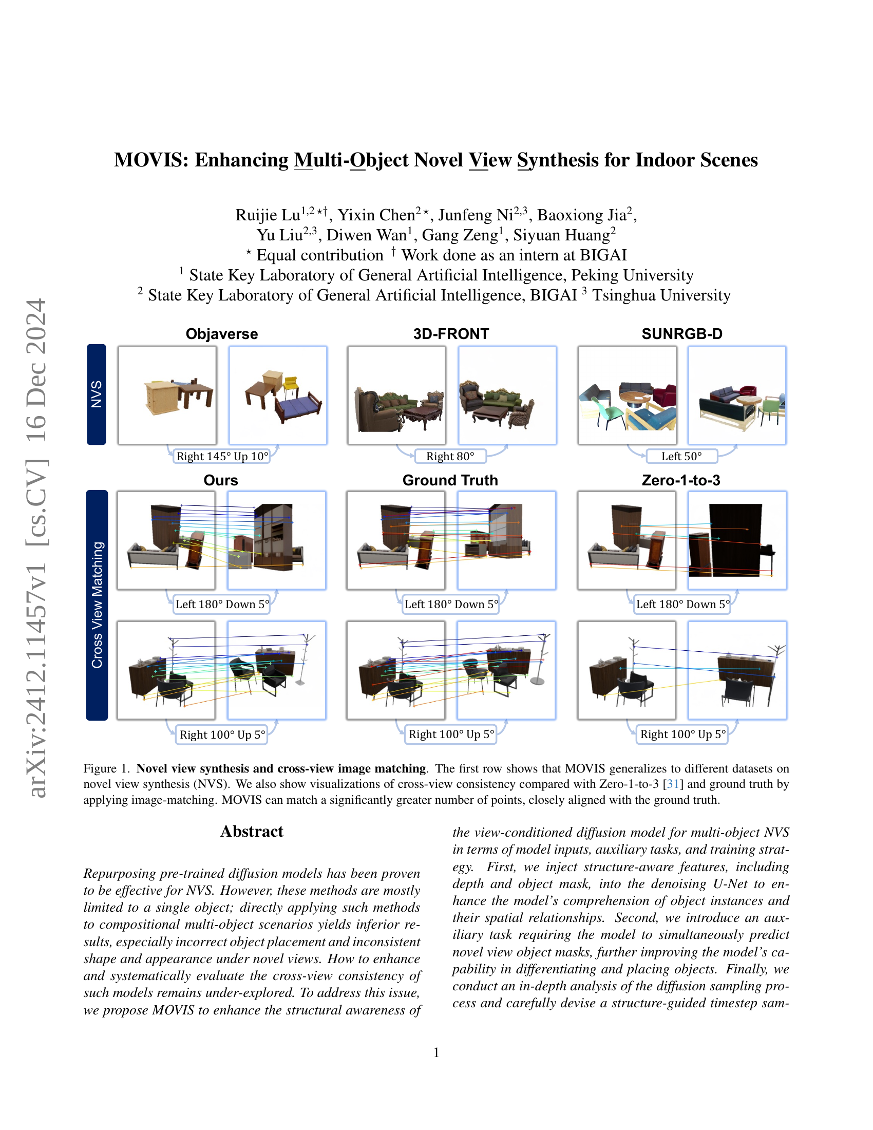
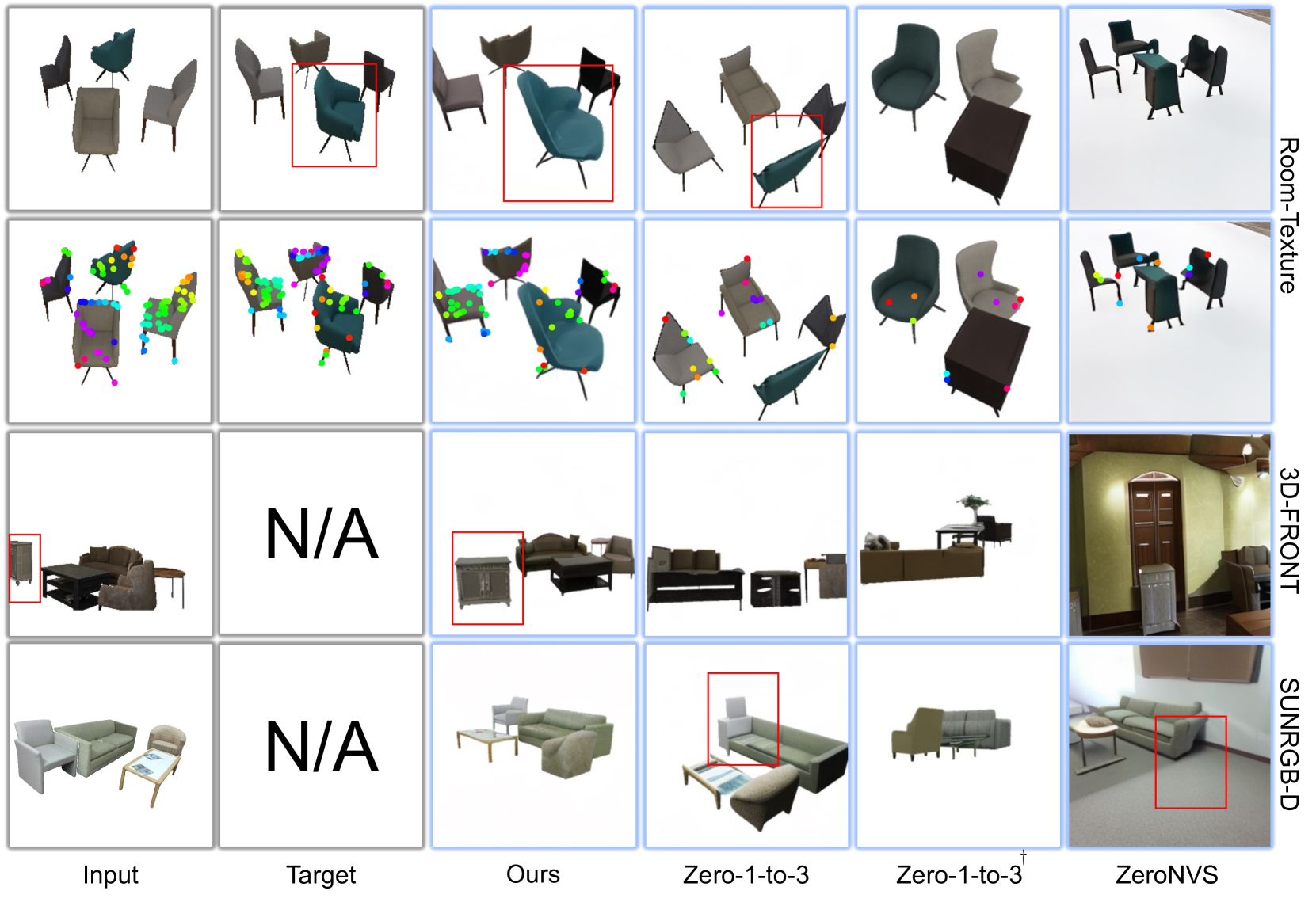
🔼 Figure 1 showcases the effectiveness of MOVIS, a novel view synthesis method, across various datasets (Objaverse, 3D-FRONT, SUNRGB-D) and compares its performance against Zero-1-to-3 and ground truth. The top row demonstrates NVS results, highlighting MOVIS’s ability to generate realistic novel views of multi-object scenes. The bottom two rows focus on cross-view consistency, showing how well the generated views align with the input view through image matching. MOVIS consistently matches a higher number of points and closely aligns with the ground truth compared to Zero-1-to-3, indicating improved structural and appearance consistency across different viewpoints.
read the caption
Figure 1: \Aclnvs and cross-view image matching. The first row shows that MOVIS generalizes to different datasets on NVS. We also show visualizations of cross-view consistency compared with Zero-1-to-3 [31] and ground truth by applying image-matching. MOVIS can match a significantly greater number of points, closely aligned with the ground truth.
| Dataset | Method | PSNR(↑) | SSIM(↑) | LPIPS(↓) | Placement(IoU(↑)) | Cross-view Consistency(Hit Rate(↑)) | Cross-view Consistency(Dist(↓)) |
|---|---|---|---|---|---|---|---|
| C3DFS | ZeroNVS | 10.704 | 0.533 | 0.481 | 21.6 | 1.2 | 130.3 |
| C3DFS | Zero-1-to-3 | 14.255 | 0.771 | 0.302 | 33.7 | 5.8 | 86.9 |
| C3DFS | Zero-1-to-3† | 14.811 | 0.794 | 0.283 | 34.4 | 1.6 | 120.3 |
| C3DFS | Ours | 17.432 | 0.825 | 0.171 | 58.1 | 37.0 | 44.8 |
| Room-Texture | ZeroNVS | 8.217 | 0.647 | 0.487 | 8.2 | 1.2 | 140.3 |
| Room-Texture | Zero-1-to-3 | 9.860 | 0.712 | 0.406 | 13.9 | 2.9 | 104.1 |
| Room-Texture | Zero-1-to-3† | 8.342 | 0.657 | 0.452 | 13.5 | 0.5 | 157.4 |
| Room-Texture | Ours | 10.014 | 0.718 | 0.366 | 24.2 | 6.1 | 78.1 |
| Objaverse | ZeroNVS | 10.557 | 0.513 | 0.486 | 17.3 | 2.3 | 126.9 |
| Objaverse | Zero-1-to-3 | 15.850 | 0.810 | 0.259 | 34.7 | 10.7 | 80.7 |
| Objaverse | Zero-1-to-3† | 15.433 | 0.815 | 0.273 | 29.7 | 1.7 | 126.7 |
| Objaverse | Ours | 17.749 | 0.840 | 0.169 | 51.3 | 50.0 | 47.2 |
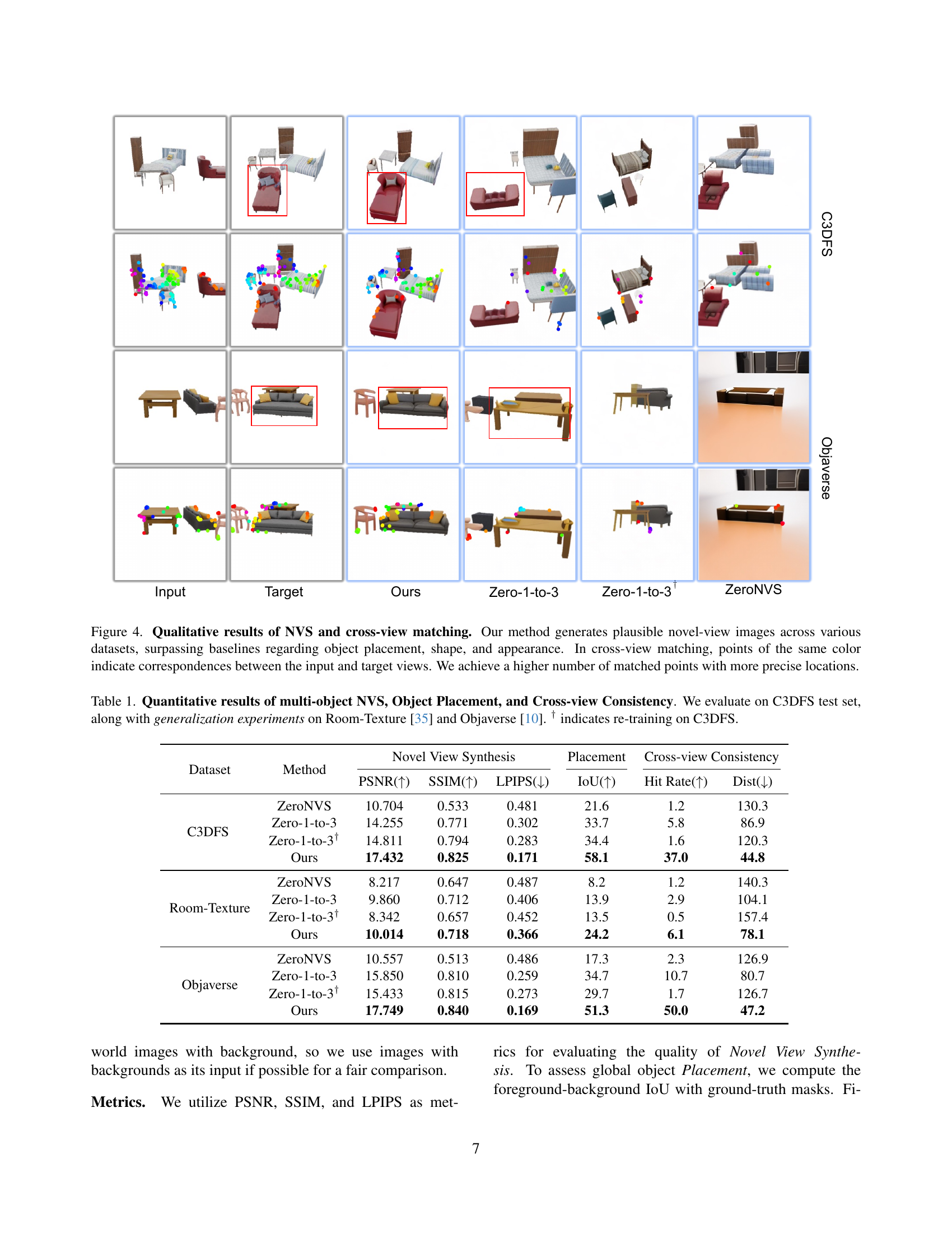
🔼 This table presents quantitative results comparing the proposed MOVIS method with ZeroNVS and Zero-1-to-3 (with and without retraining on C3DFS) across three datasets: C3DFS, Room-Texture, and Objaverse. Metrics include PSNR, SSIM, and LPIPS for novel view synthesis quality, Intersection over Union (IoU) for object placement accuracy, and Hit Rate and average matching distance (Dist) for cross-view consistency. Higher values are better for PSNR, SSIM, IoU, and Hit Rate, while lower values are better for LPIPS and Dist.
read the caption
Table 1: Quantitative results of multi-object NVS, Object Placement, and Cross-view Consistency. We evaluate on C3DFS test set, along with generalization experiments on Room-Texture [35] and Objaverse [10]. † indicates re-training on C3DFS.
In-depth insights#
Structure-Aware NVS#
Structure-aware Novel View Synthesis (NVS) focuses on generating novel views of a scene while preserving its 3D structure. This is crucial for realistic and consistent image synthesis, especially in complex multi-object scenarios. Traditional methods often struggle with object placement, distortion, and inconsistencies under novel viewpoints. Structure-aware approaches aim to mitigate these issues by incorporating explicit 3D information, such as depth maps and object masks. By leveraging such structural cues, these NVS models can better understand object relationships and spatial layouts within the scene, leading to more plausible and coherent novel view images. Furthermore, predicting object masks in the novel view serves as a useful auxiliary task to guide the model’s structure learning and object placement capabilities. Evaluating cross-view consistency through image-matching provides a robust measure of how well the generated views maintain structural integrity compared to the input. This approach marks a significant step towards enabling more realistic and consistent multi-object NVS.
Guided Timestep Sampling#
Guided timestep sampling enhances diffusion models for novel view synthesis by strategically selecting timesteps during training. Larger timesteps prioritize global object placement, crucial for multi-object scenes, while smaller timesteps refine detailed geometry and appearance. This balancing act addresses the inherent complexity of multi-object scenarios, yielding more plausible and consistent novel views. This method offers a significant advancement in synthesizing complex scenes.
Cross-View Consistency#
Cross-view consistency is crucial for multi-object novel view synthesis (NVS). It ensures plausible object placement, shape, and appearance across different viewpoints. The paper introduces image-matching techniques to quantify this consistency, measuring how well-matched points align between synthesized and ground truth images. This approach provides a more robust evaluation than traditional image-level metrics, directly addressing the challenge of maintaining structural integrity in complex scenes. By focusing on cross-view consistency, the research aims to enhance realism and reduce artifacts in multi-object NVS, paving the way for more realistic and immersive 3D experiences.
Multi-Object NVS Limits#
Multi-object Novel View Synthesis (NVS) faces inherent limits. Synthesizing plausible novel views of multiple objects requires a deep understanding of complex scene structure. This encompasses object placement, geometry, and their inter-relationships. Current methods struggle due to several factors. Firstly, occlusion poses a challenge, as objects may partially or completely obstruct one another. Accurately predicting the appearance of occluded regions necessitates strong 3D reasoning. Secondly, the interaction of light and shadow within a multi-object scene adds complexity. The interplay of light sources and object placement produces intricate shadow patterns that are difficult to model realistically. Thirdly, view consistency becomes more critical in multi-object scenes. As the viewpoint changes, the model must maintain object permanence, ensuring that objects remain consistent in shape and appearance across various views. Failure to address view consistency leads to visual artifacts and inconsistencies, breaking the illusion of realism. Addressing these limitations demands further research, potentially focusing on improved 3D representation, more sophisticated occlusion handling, and better techniques for modeling lighting effects.
Diffusion Model Gen.#
Diffusion Model Gen. likely refers to generative diffusion models, a powerful class of models capable of synthesizing high-quality images. These models learn by progressively adding noise to training images until they become pure noise, and then learning to reverse this process to generate new images from random noise. Key strengths include high-quality output and diverse sample generation. However, they can be computationally expensive during both training and inference. Further research focuses on improving sampling efficiency and incorporating conditional information to control the generation process, enabling tasks like novel view synthesis and image editing explored in the paper.
More visual insights#
More on figures

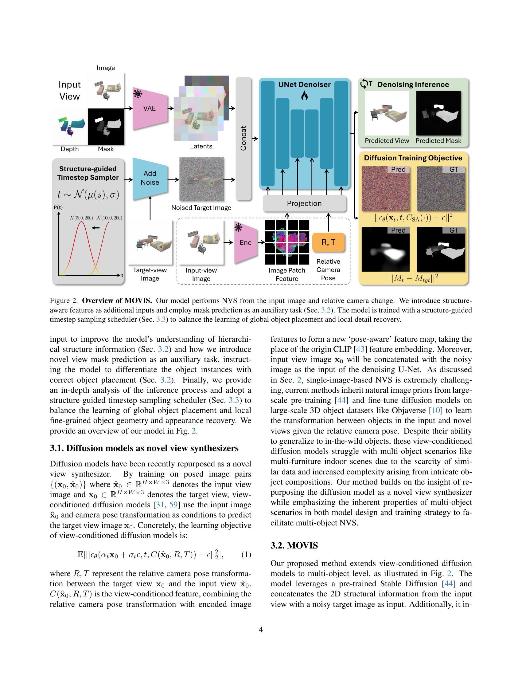
🔼 MOVIS performs novel view synthesis by taking an input image and relative camera change as input. It incorporates structure-aware features (depth and object mask) and predicts a novel view mask as an auxiliary task. The model uses a structure-guided timestep sampling scheduler to balance learning global object placement and local detail recovery.
read the caption
Figure 2: Overview of MOVIS. Our model performs NVS from the input image and relative camera change. We introduce structure-aware features as additional inputs and employ mask prediction as an auxiliary task (Sec. 3.2). The model is trained with a structure-guided timestep sampling scheduler (Fig. 3) to balance the learning of global object placement and local detail recovery.

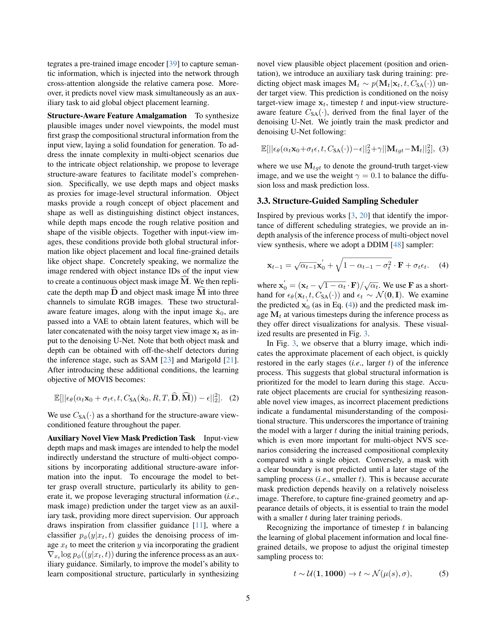
🔼 This figure visualizes the inference process of a diffusion model for novel view synthesis, demonstrating how object placement and mask prediction evolve during denoising. Early inference steps (large t) prioritize global object placement, resulting in blurry object shapes. Later steps (small t) refine object details and produce sharper masks. The visualization compares models trained with and without a ‘shifted’ timestep sampling scheduler. The shifted scheduler prioritizes larger t initially, gradually decreasing, allowing the model to first learn object placement, then fine-grained details and mask prediction. Results show that training with a shifted scheduler leads to better mask predictions and more detailed object reconstructions. The images of the chair visualize how the prediction of object and the object mask are evolving at different time steps.
read the caption
Figure 3: Visualization of inference. The early stage of the denoising process focuses on restoring global object placements, while the prediction of object masks requires a relatively noiseless image to recover fine-grained geometry. This motivates us to seek a balanced timestep sampling scheduler during training. The model trained w/ shift yields better mask prediction and thus recovers an image with more details and sharp object boundary. The w/o shift here refers to not shifting the μ𝜇\muitalic_μ value.

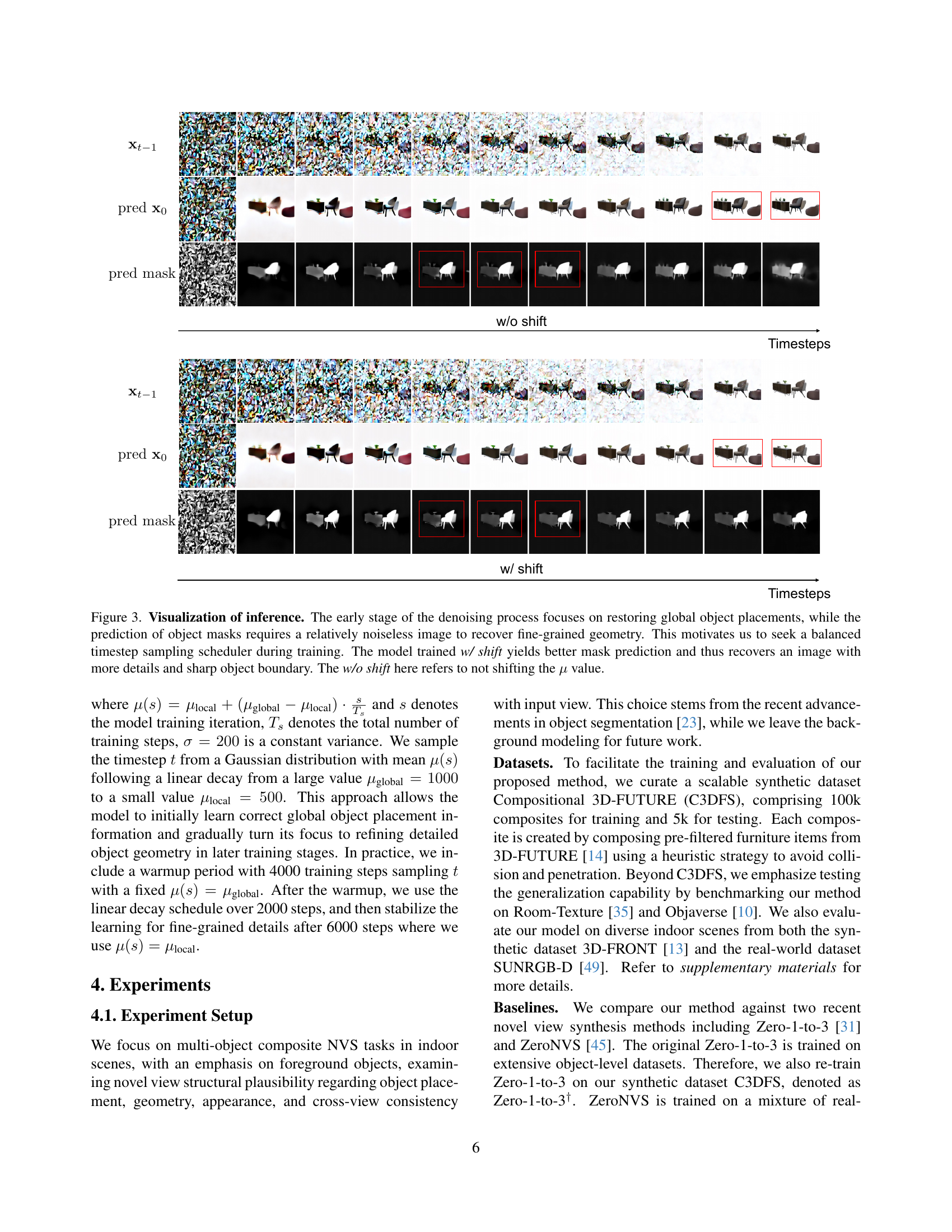
🔼 This figure presents qualitative results of Novel View Synthesis (NVS) generated by the proposed MOVIS model, compared to baseline models (Zero-1-to-3, Zero-1-to-3+, and ZeroNVS) on three different datasets: C3DFS, Objaverse and an unspecified dataset. The first column displays input images, the second shows target images (ground truth), and the subsequent columns show results generated by each method. The figure demonstrates that MOVIS generates more plausible images compared to other methods, particularly in terms of object placement, shape, and appearance. This figure also includes visualizations of cross-view image matching, where points of the same color connect corresponding features between input and novel view images. The results demonstrate that MOVIS achieves more and precise matches compared to baselines, further indicating improved cross-view consistency.
read the caption
Figure 4: Qualitative results of NVS and cross-view matching. Our method generates plausible novel-view images across various datasets, surpassing baselines regarding object placement, shape, and appearance. In cross-view matching, points of the same color indicate correspondences between the input and target views. We achieve a higher number of matched points with more precise locations.

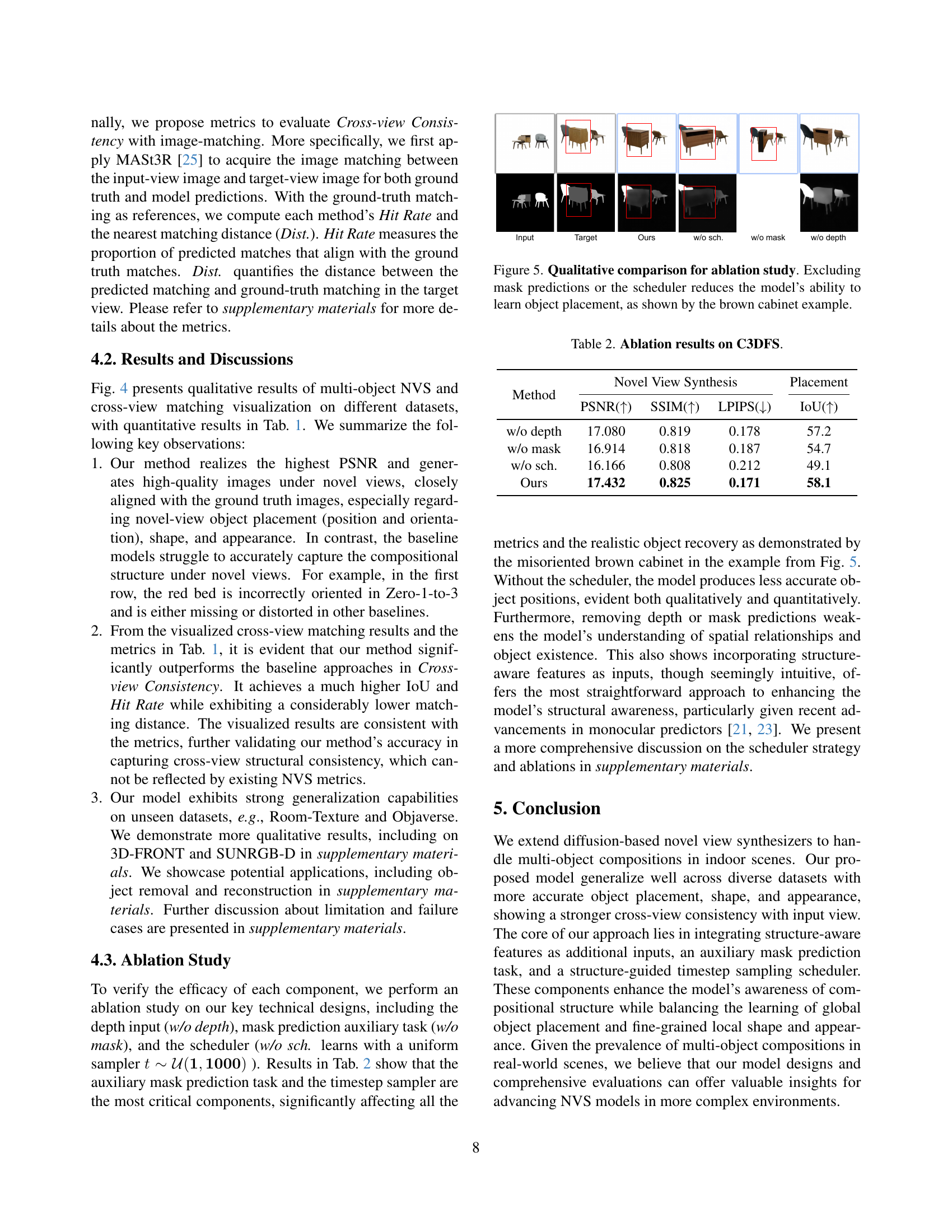
🔼 This figure presents a qualitative comparison of the results obtained from different ablation settings of the proposed MOVIS model. The ablations involve removing specific components of the model, such as the structure-aware features (depth and mask), the auxiliary mask prediction task, and the structure-guided timestep sampling scheduler. The figure showcases the impact of each component on the model’s performance, particularly in terms of object placement, shape, and appearance in novel view synthesis. The ‘w/o shift’ label indicates the use of a uniform timestep sampling strategy, as described in the main paper. The visualizations demonstrate that both the auxiliary mask prediction task and the timestep sampler are crucial components of the model, significantly impacting the accuracy of object placement. As shown in the example of the brown cabinet, excluding either of these components leads to noticeably incorrect or distorted object orientations.
read the caption
Figure 5: Qualitative comparison for ablation study. Excluding mask predictions or the scheduler reduces the model’s ability to learn object placement, as shown by the brown cabinet example.
🔼 This figure illustrates three different timestep sampling strategies, which determine how the timestep t is sampled during the training process of the diffusion model. The x-axis represents training steps, while the y-axis represents the mean (μ) of the Gaussian distribution from which t is sampled. The variance is fixed at 200. The orange line represents the KMS (Keeping Mean Static) strategy, where the mean is kept constant at 1000. The blue line stands for LIND (Linear Increase and Decline). It starts with the mean at 1000 and linearly decreases it to 500 until 6000 steps before keeping it static. The green line shows LDC (Linear Decline Common Parts), where the mean starts at 1000 and linearly declines to 500. This is also visually represented in the paper’s Figure 3.
read the caption
Figure S.6: Illustration of different timestep sampling strategies.
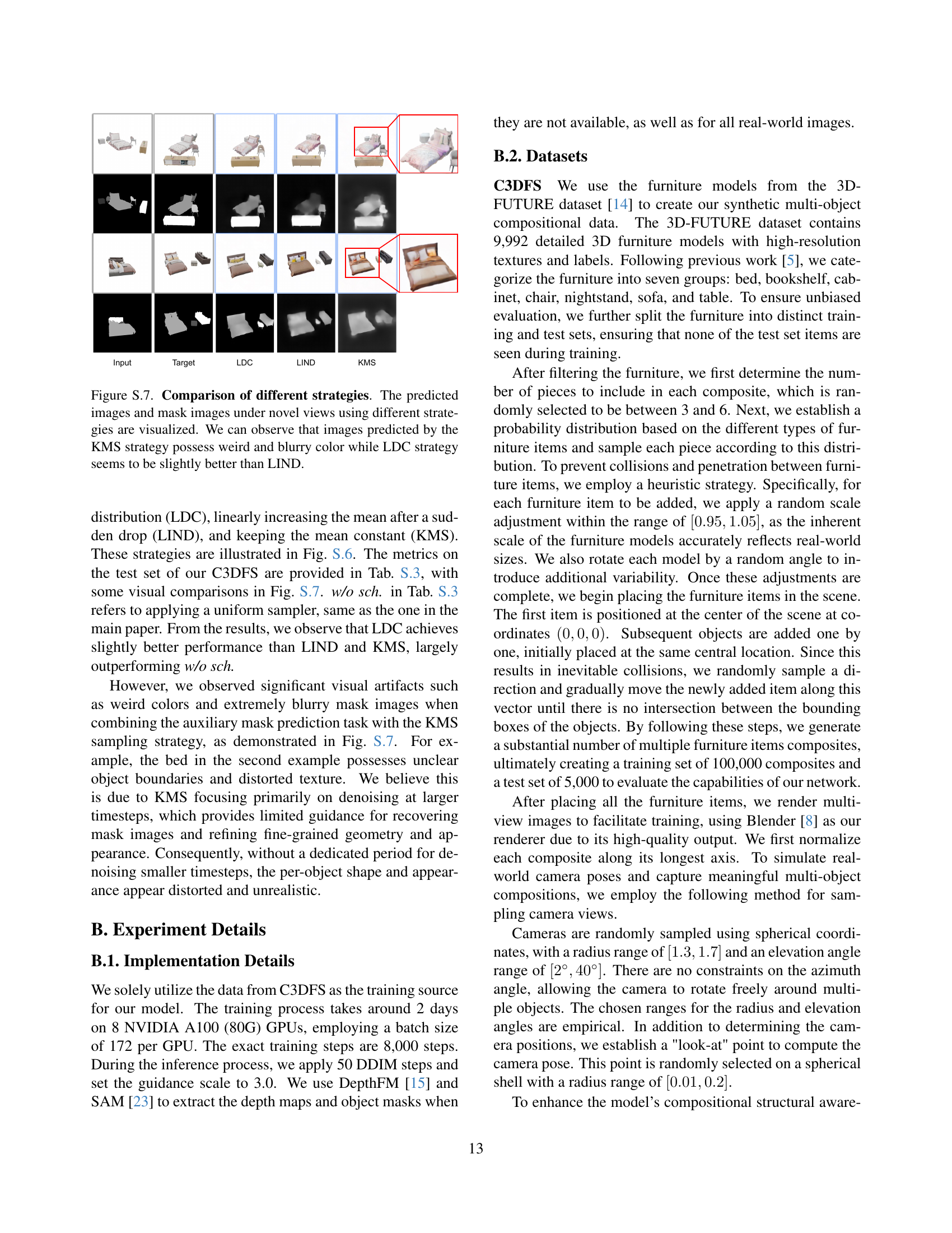
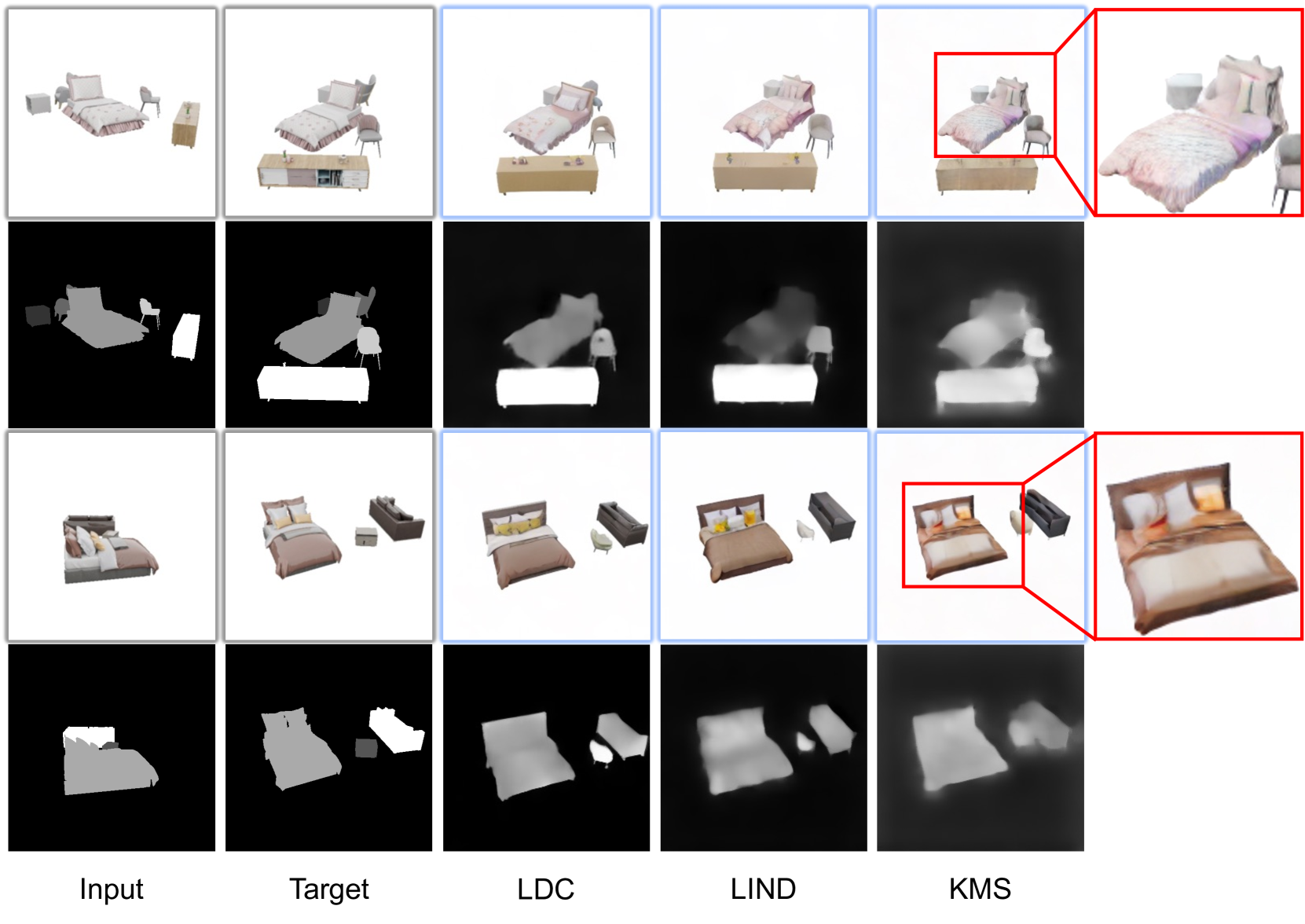
🔼 This figure shows a comparison of novel view synthesis results using different timestep sampling strategies during the denoising diffusion process. Images and predicted masks under novel viewpoints are displayed for KMS (constant mean), LIND (linear increasing after drop), and LDC (linearly decreasing mean) strategies. The input, target, and predicted images, along with the predicted object masks, are presented for each strategy. Qualitative differences can be observed, particularly in color and mask sharpness. Images generated with KMS exhibit unnatural colors and blurry masks. LDC generally produces sharper and more realistic novel view images compared to LIND and KMS.
read the caption
Figure S.7: Comparison of different strategies. The predicted images and mask images under novel views using different strategies are visualized. We can observe that images predicted by the KMS strategy possess weird and blurry color while LDC strategy seems to be slightly better than LIND.

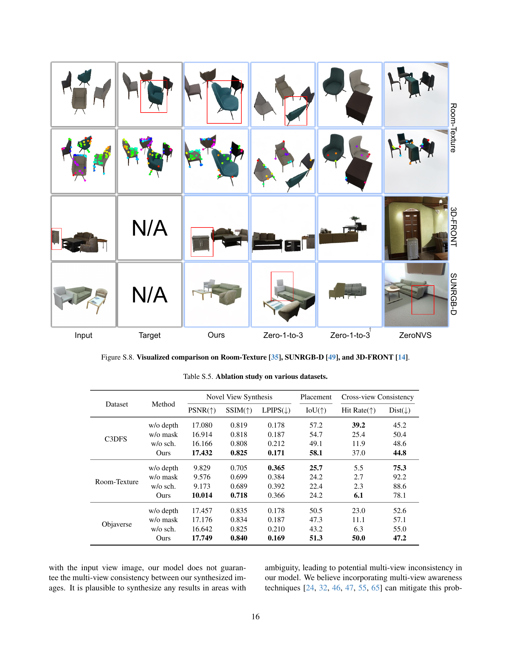
🔼 This figure presents a visual comparison of the proposed method’s performance against baseline models on three datasets: Room-Texture, SUNRGB-D, and 3D-FRONT. Each dataset showcases various indoor scenes with multiple objects. For each scene, the input image, target image, the results generated by the proposed method, Zero-1-to-3, Zero-1-to-3+ and ZeroNVS are presented along with their corresponding predicted object masks. Note: ‘N/A’ indicates that the specific viewpoint is not available in the dataset.
read the caption
Figure S.8: Visualized comparison on Room-Texture [35], SUNRGB-D [49], and 3D-FRONT [14].

🔼 This figure illustrates the model’s capability to synthesize plausible novel views of multi-object indoor scenes from various camera positions. Each block of images demonstrates the NVS results for a single scene. The top part of each block showcases the randomly sampled camera viewpoints and their corresponding synthesized images. The bottom part displays the input image (leftmost), a predicted novel view image (middle), and the ground-truth novel view image (rightmost). The first five examples (first five rows) use scenes from the SUNRGB-D dataset, and the last three examples (last three rows) use scenes from the 3D-FRONT dataset. The figure emphasizes the model’s capability in maintaining the geometry and structure of the objects under novel view points and demonstrate the novel view synthesis quality of the proposed model.
read the caption
Figure S.9: Continuous rotation examples on SUNRGB-D and 3D-FRONT. We rotate the camera around the multi-object composites, successfully synthesizing plausible novel-view images across a wide range of camera pose variations. This first five examples are from SUNRGB-D, and the last three examples are from 3D-FRONT.

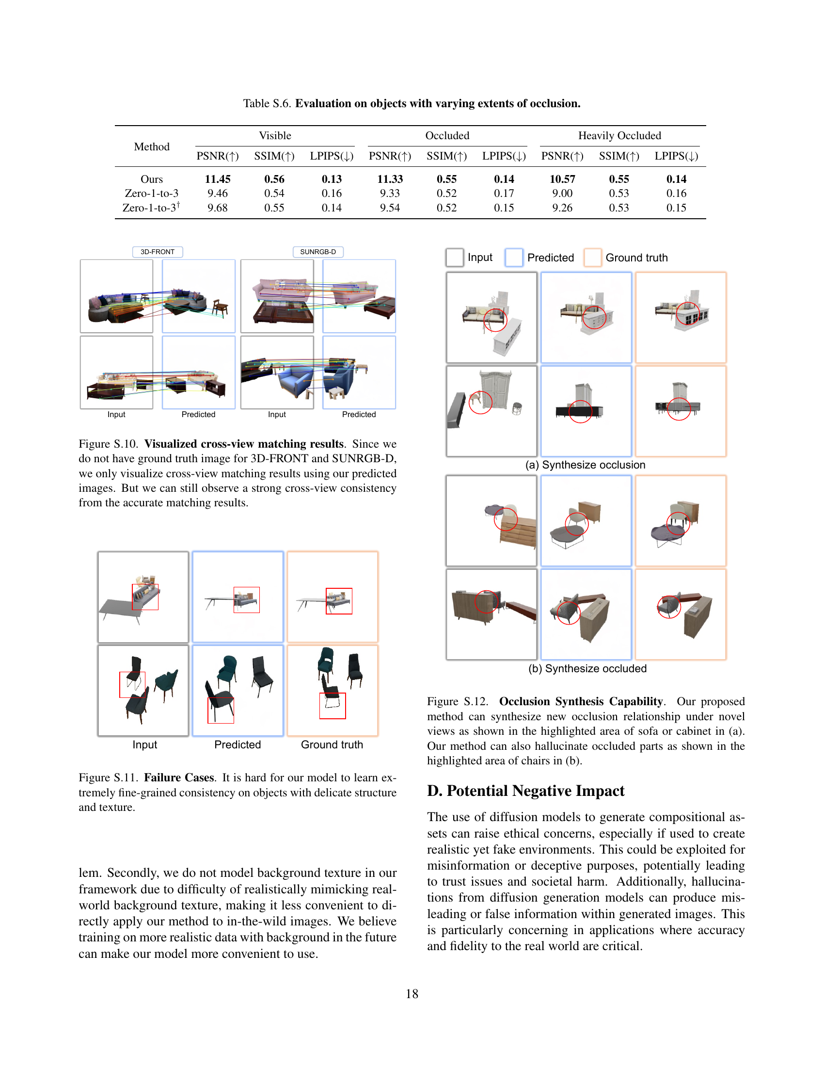
🔼 This figure visualizes the cross-view matching results produced by the proposed model on the 3D-FRONT and SUNRGB-D datasets. Since ground truth images are not available for these datasets for comparison, the matching is performed using the model’s predicted images. Despite the lack of ground truth, the results exhibit strong cross-view consistency as indicated by accurate matching points. The visualizations showcase the model’s capability to maintain consistent object placement and shape across different viewpoints, even without access to ground truth data. The top image uses 3D-FRONT data and the bottom image uses SUNRGB-D data.
read the caption
Figure S.10: Visualized cross-view matching results. Since we do not have ground truth image for 3D-FRONT and SUNRGB-D, we only visualize cross-view matching results using our predicted images. But we can still observe a strong cross-view consistency from the accurate matching results.

🔼 This figure showcases two failure cases of the proposed model for novel view synthesis. The first example focuses on a sofa with colorful pillows, where the model struggles to accurately capture the delicate texture and structure of the pillows. Although the overall placement of the sofa is reasonable, the fine-grained details are not consistent with the ground truth. The second example features chairs with slim legs. Similar to the first case, the model’s prediction is approximately correct regarding chair placement, but it fails to perfectly synthesize the slim legs, resulting in a less realistic appearance compared to the target image. These examples highlight the model’s limitation in learning extremely fine-grained consistency on objects with complex structures and textures.
read the caption
Figure S.11: Failure Cases. It is hard for our model to learn extremely fine-grained consistency on objects with delicate structure and texture.

🔼 This figure demonstrates the model’s ability to handle object occlusions. Subfigure (a) showcases the model’s capacity to generate novel view images with plausible occlusions that were not present in the original input view. Specifically, the highlighted area of the sofa and cabinet demonstrates the model generating appropriate occlusion relationships in the novel view, showing the sofa arm correctly occluding the side of the cabinet, even though the cabinet’s side is visible in the original view. Subfigure (b) illustrates the model’s ability to hallucinate previously occluded object parts in the novel view. The highlighted chairs are shown completely, including the parts occluded by the table in the input view. Thus, the figure conveys that the model can create plausible occlusions in new viewpoints and fill in missing information for previously hidden objects.
read the caption
Figure S.12: Occlusion Synthesis Capability. Our proposed method can synthesize new occlusion relationship under novel views as shown in the highlighted area of sofa or cabinet in (a). Our method can also hallucinate occluded parts as shown in the highlighted area of chairs in (b).

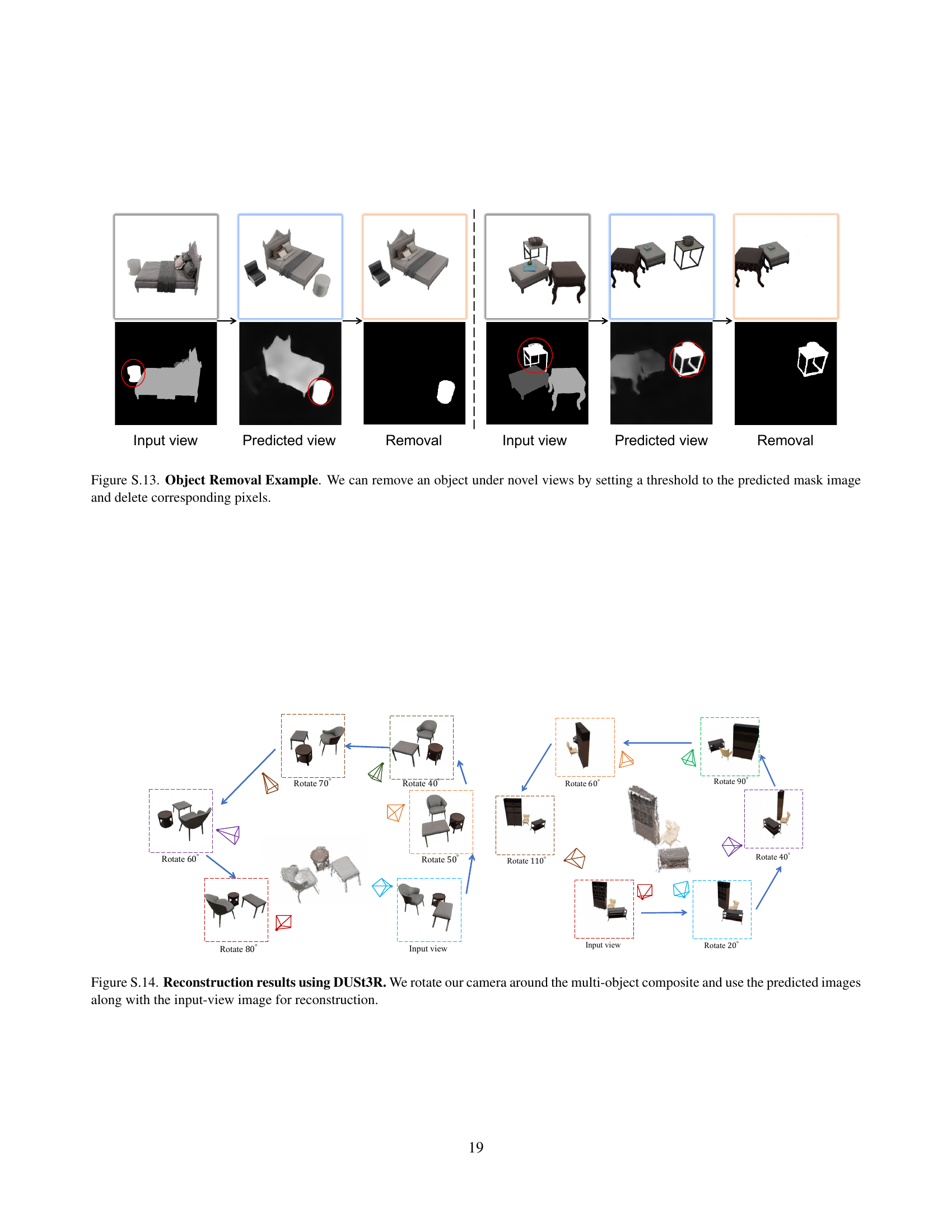
🔼 This figure showcases the object removal capabilities of the proposed model under novel viewpoints. In the first example, the method successfully removes the pillows from the bed by setting a threshold to the predicted mask image and masking out corresponding pixels. Similarly, in the second example, the table is removed from the scene. This demonstrates that by using the predicted mask image, it’s possible to remove an object in the novel view image as if it was never there.
read the caption
Figure S.13: Object Removal Example. We can remove an object under novel views by setting a threshold to the predicted mask image and delete corresponding pixels.

🔼 This figure showcases 3D reconstruction results derived from novel view images generated by the proposed model, MOVIS, using an off-the-shelf 3D reconstruction method, DUSt3R [58]. The top row depicts a bedroom scene, while the bottom row represents a living room. In both scenarios, the input view image is provided alongside multiple novel view images generated by MOVIS. These novel views, along with the original input view, are then used as input for DUSt3R to reconstruct the 3D scene. This demonstrates the potential application of MOVIS in 3D scene reconstruction tasks. The relative camera pose between each novel-view image and the input-view image is visualized with arrows and rotation angles.
read the caption
Figure S.14: Reconstruction results using DUSt3R. We rotate our camera around the multi-object composite and use the predicted images along with the input-view image for reconstruction.

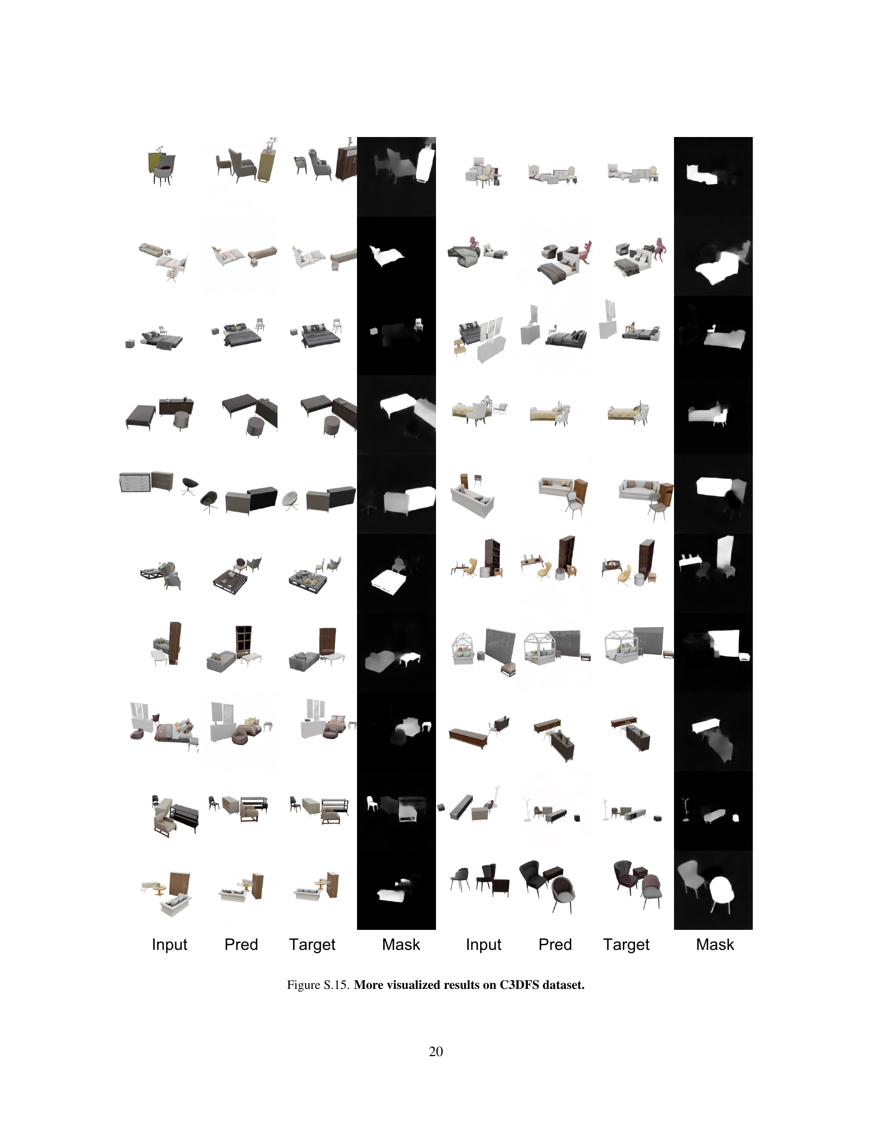
🔼 This figure supplements Figure 4 in the main paper, providing more visualized results of the proposed model’s novel view synthesis capabilities on the Compositional 3D-FUTURE (C3DFS) dataset. Each row showcases a different multi-object scene. From left to right, the columns display the input image, the predicted novel view image, the target novel view image (ground truth), and the predicted object mask for the novel view. The figure demonstrates the model’s ability to generate plausible and consistent novel views, with accurate placement and appearance of objects in the scene, as compared to the ground truth. The inclusion of the predicted mask visualization further showcases the model’s object-level understanding.
read the caption
Figure S.15: More visualized results on C3DFS dataset.
More on tables
| Method | Novel View Synthesis | Placement | |
|---|---|---|---|
| PSNR(↑) | SSIM(↑) | LPIPS(↓) | |
| w/o depth | 17.080 | 0.819 | 0.178 |
| w/o mask | 16.914 | 0.818 | 0.187 |
| w/o sch. | 16.166 | 0.808 | 0.212 |
| Ours | 17.432 | 0.825 | 0.171 |
🔼 This table presents the ablation study results on the Compositional 3D-FUTURE (C3DFS) dataset to evaluate the effectiveness of each proposed component within the MOVIS model. These components include: - Depth input (w/o depth): Evaluates performance when depth information is excluded. - Mask prediction (w/o mask): Evaluates performance when the auxiliary mask prediction task is not used. - Scheduler (w/o sch.): Evaluates performance using a standard uniform timestep sampler t~U(1, 1000) instead of the proposed structure-guided scheduler. The table compares the performance of each ablated version against the full MOVIS model across four metrics: - PSNR (Peak Signal-to-Noise Ratio) - SSIM (Structural Similarity Index) - LPIPS (Learned Perceptual Image Patch Similarity) - IoU (Intersection over Union) for object placement. Higher PSNR, SSIM, and IoU values indicate better performance, while lower LPIPS is desirable.
read the caption
Table 2: Ablation results on C3DFS.
| Dataset | Method | Novel View Synthesis | ||
|---|---|---|---|---|
| PSNR(↑) | SSIM(↑) | LPIPS(↓) | ||
| C3DFS | w/o sch. | 16.166 | 0.808 | 0.212 |
| KMS | 17.148 | 0.823 | 0.175 | |
| LIND | 17.279 | 0.824 | 0.172 | |
| LDC | 17.432 | 0.825 | 0.171 |
🔼 This table presents an ablation study on different timestep sampling strategies for training the diffusion model in multi-object novel view synthesis. It evaluates the impact of four different sampling strategies including a uniform sampler, Karras et al. 11, linearly increasing the mean after sudden drop (LIND), and linear declining scheduler (LDC) on novel view synthesis quality and object placement accuracy. The evaluation metrics include PSNR, SSIM, LPIPS for image quality, and IoU for object placement. The results show that incorporating sampling strategies significantly improves performance, with LDC achieving the best results across all metrics.
read the caption
Table S.3: Ablation on different strategies. Incorporating sampling strategies significantly improves the model performance, while the linear decline (LDC) achieves the best.
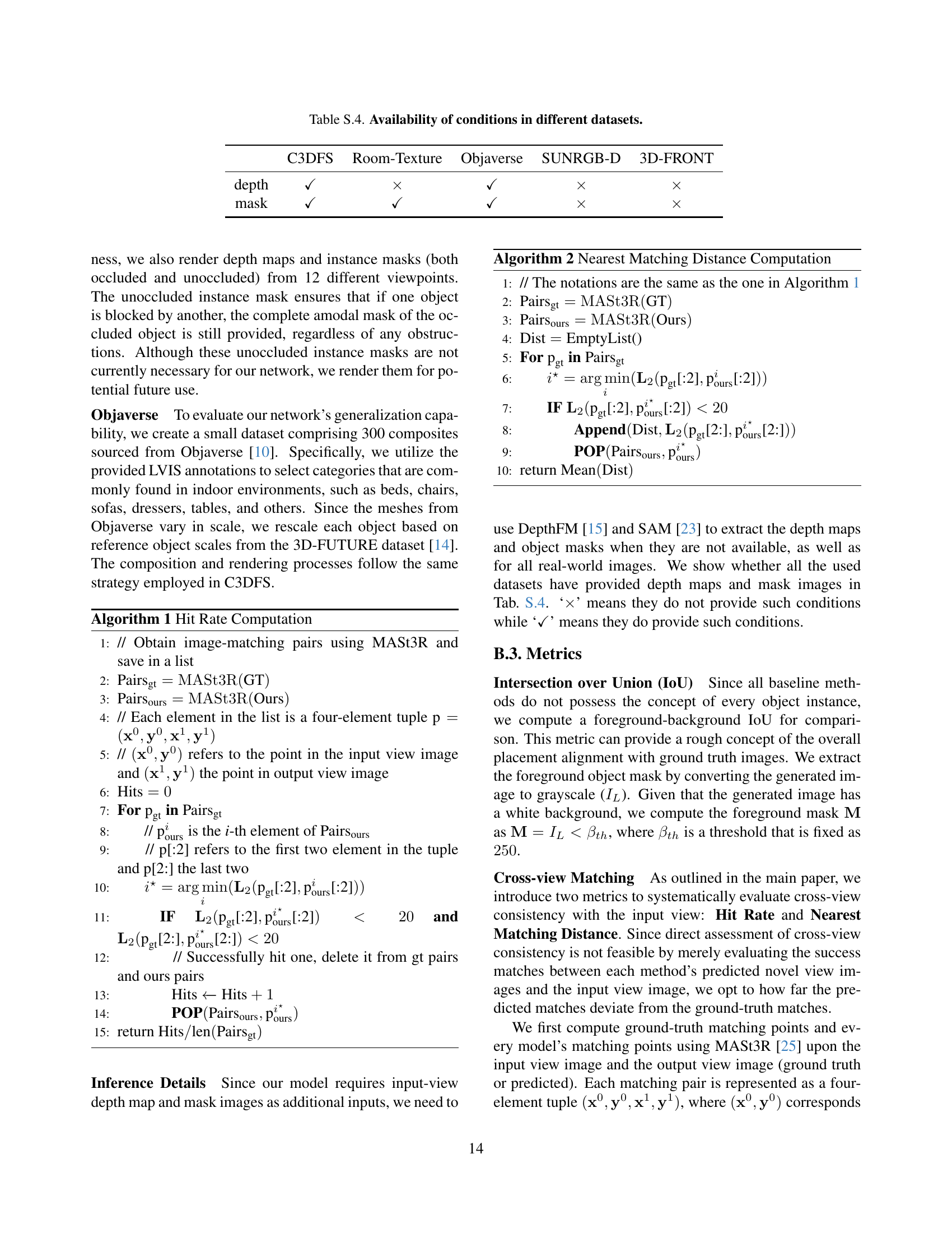
| C3DFS | Room-Texture | Objaverse | SUNRGB-D | 3D-FRONT | |
|---|---|---|---|---|---|
| depth | ✓ | × | ✓ | × | × |
| mask | ✓ | ✓ | ✓ | × | × |
🔼 This table indicates whether depth and mask information are provided by default in the five datasets used in this paper (C3DFS, Room-Texture, Objaverse, SUNRGB-D, and 3D-FRONT). An ‘x’ indicates that the dataset does not inherently provide the information, while a checkmark indicates that it does.
read the caption
Table S.4: Availability of conditions in different datasets.
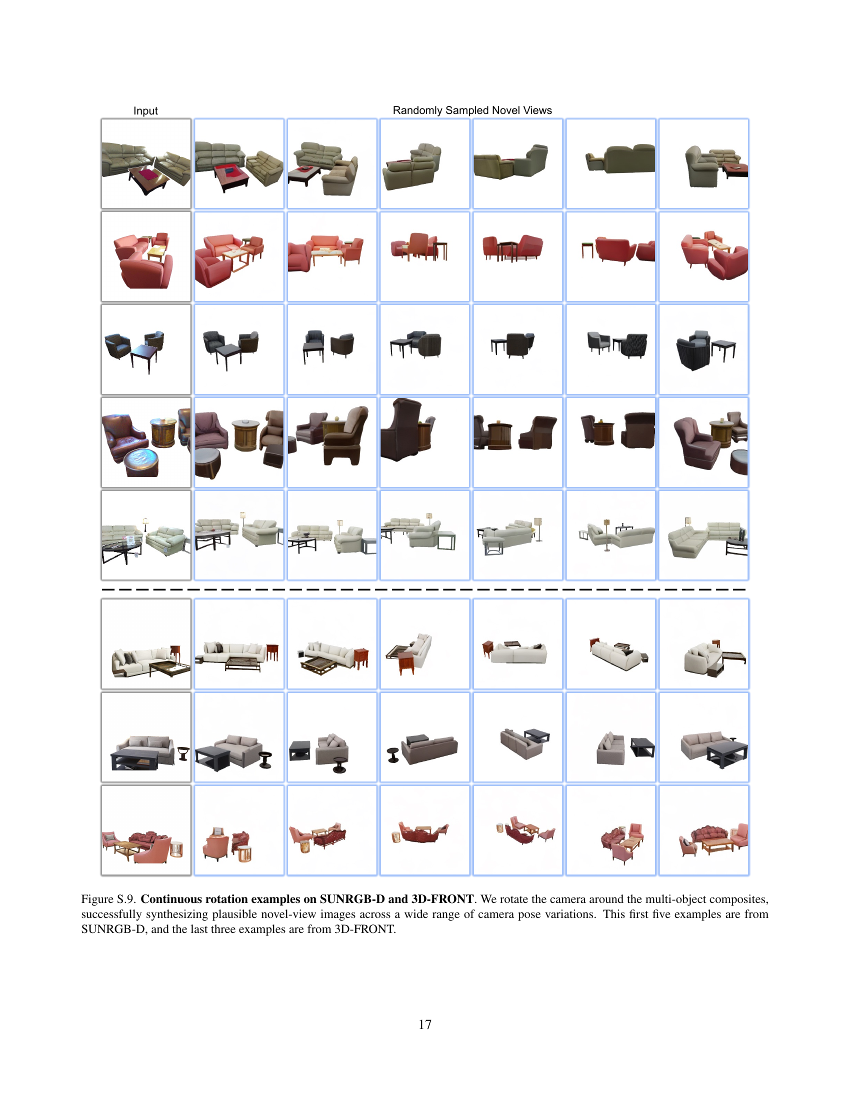
| Dataset | Method | Novel View Synthesis | Placement | Cross-view Consistency |
|---|---|---|---|---|
| PSNR(↑) | SSIM(↑) | LPIPS(↓) | ||
| C3DFS | w/o depth | 17.080 | 0.819 | 0.178 |
| w/o mask | 16.914 | 0.818 | 0.187 | |
| w/o sch. | 16.166 | 0.808 | 0.212 | |
| Ours | 17.432 | 0.825 | 0.171 | |
| Room-Texture | w/o depth | 9.829 | 0.705 | 0.365 |
| w/o mask | 9.576 | 0.699 | 0.384 | |
| w/o sch. | 9.173 | 0.689 | 0.392 | |
| Ours | 10.014 | 0.718 | 0.366 | |
| Objaverse | w/o depth | 17.457 | 0.835 | 0.178 |
| w/o mask | 17.176 | 0.834 | 0.187 | |
| w/o sch. | 16.642 | 0.825 | 0.210 | |
| Ours | 17.749 | 0.840 | 0.169 |
🔼 This table presents the ablation study results of the proposed method on three datasets: C3DFS, Room-Texture, and Objaverse. The ablation study is conducted by removing one component at a time including depth input, mask prediction, and sampling scheduler, to evaluate the individual contribution of each component to the model’s performance in novel view synthesis. The evaluation metrics include PSNR, SSIM, LPIPS for image quality, IoU for object placement accuracy, Hit Rate and average nearest matching distance (Dist) for cross-view consistency.
read the caption
Table S.5: Ablation study on various datasets.
| Method | Visible | Occluded | Heavily Occluded | |||||||
|---|---|---|---|---|---|---|---|---|---|---|
| PSNR(↑) | SSIM(↑) | LPIPS(↓) | PSNR(↑) | SSIM(↑) | LPIPS(↓) | PSNR(↑) | SSIM(↑) | LPIPS(↓) | ||
| — | — | — | — | — | — | — | — | — | — | — |
| Ours | 11.45 | 0.56 | 0.13 | 11.33 | 0.55 | 0.14 | 10.57 | 0.55 | 0.14 | |
| Zero-1-to-3 | 9.46 | 0.54 | 0.16 | 9.33 | 0.52 | 0.17 | 9.00 | 0.53 | 0.16 | |
| Zero-1-to-3† | 9.68 | 0.55 | 0.14 | 9.54 | 0.52 | 0.15 | 9.26 | 0.53 | 0.15 |
🔼 This table evaluates the performance of different novel view synthesis models on objects with varying levels of occlusion in the input view. It breaks down the results into three categories: objects that are fully visible, objects that are partially occluded, and objects that are heavily occluded. For each category and each method, the table reports PSNR, SSIM, and LPIPS scores, providing a comprehensive evaluation of how well the models handle different occlusion scenarios.
read the caption
Table S.6: Evaluation on objects with varying extents of occlusion.
Full paper#
