↗ arXiv ↗ Hugging Face ↗ Papers with Code
TL;DR#
Videos are complex, and analyzing them frame-by-frame ignores how frames relate to each other. Tokenization, which converts video to compact representations, addresses this by capturing temporal dynamics. However, current video tokenizers often lack open access or struggle to balance performance and flexibility. This hinders research in video-related fields like generation and understanding, where efficient representations are key. Existing methods often treat frames independently using image tokenizers. This overlooks relationships between frames. Other video-specific tokenizers may be closed-source or show limited performance. Thus, there is a need for efficient, adaptable, and publicly available tools for video tokenization. This allows researchers to build on established tools. Open access is crucial to speeding the field’s growth.
This paper introduces VidTok, a new open-source video tokenizer designed to be both versatile and high-performing. It cleverly combines 2D convolutions for spatial processing and 3D convolutions for temporal fusion. This hybrid architecture reduces computational costs without sacrificing quality. For discrete tokens, VidTok leverages Finite Scalar Quantization (FSQ), enhancing training stability. It also uses a two-stage training strategy, first training on low-resolution videos, then fine-tuning on higher resolutions. This method greatly speeds training. VidTok excels in both continuous and discrete tokenization benchmarks, beating current top performers. It is publicly available, aiming to be a cornerstone tool for future video research.
Key Takeaways#
Why does it matter?#
VidTok’s open-source nature democratizes access to cutting-edge video tools, enabling broader participation in video-centric research. It addresses the increasing need for efficient video representation learning, crucial for various applications. Its innovative architecture and training strategies offer valuable insights for model efficiency. By making state-of-the-art video tokenization widely accessible, it facilitates advancements in video generation, understanding, and other related research.
Visual Insights#

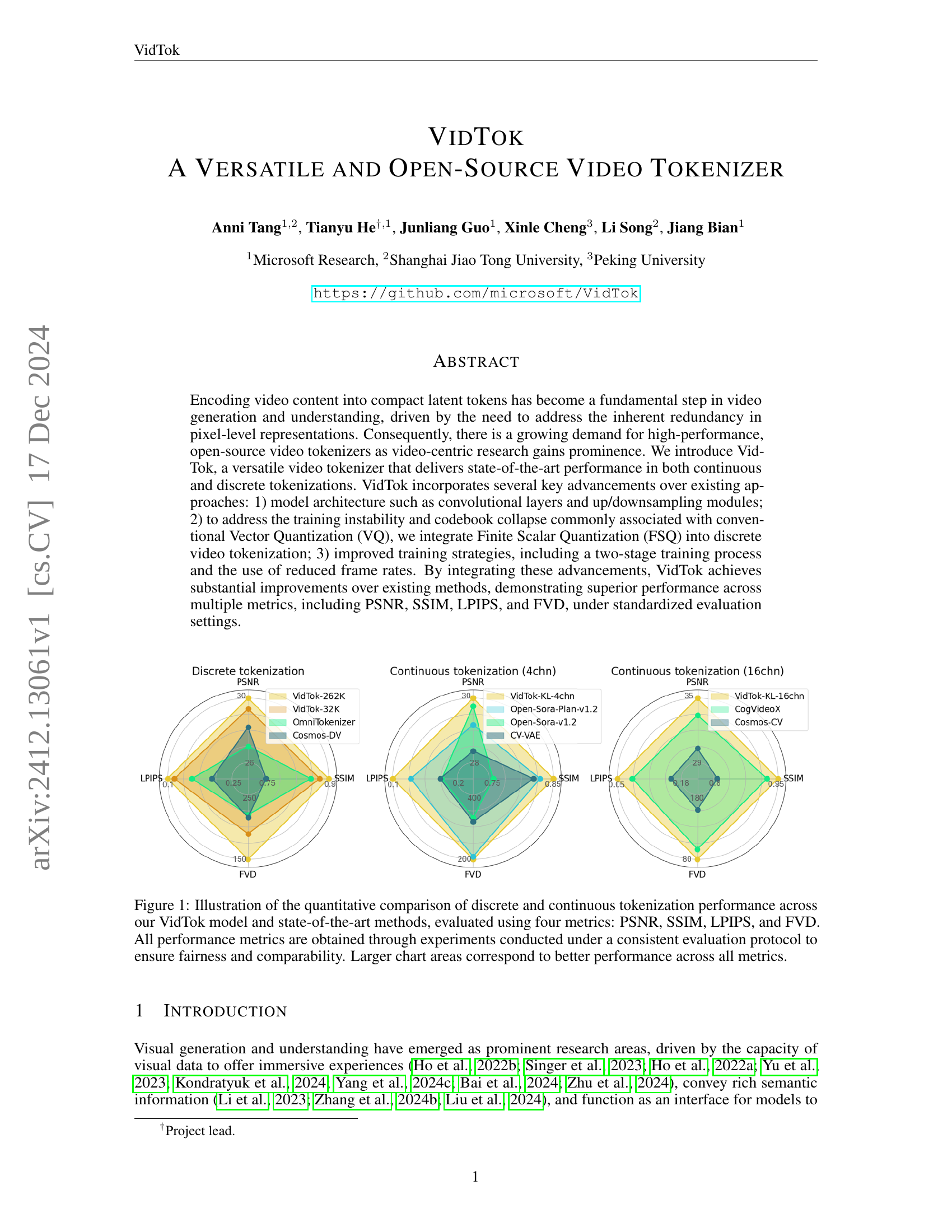
🔼 This figure provides a quantitative comparison of VidTok and other state-of-the-art video tokenizers. The comparison is split into three radar charts, one for discrete tokenization, and two for continuous tokenization (4 channel and 16 channel). Each radar chart is measured across four metrics (PSNR, SSIM, LPIPS, and FVD). The area within the radar chart polygon indicates the relative performance across each metric where a larger area denotes better performance. VidTok appears to generally outperform the other methods.
read the caption
Figure 1: Illustration of the quantitative comparison of discrete and continuous tokenization performance across our VidTok model and state-of-the-art methods, evaluated using four metrics: PSNR, SSIM, LPIPS, and FVD. All performance metrics are obtained through experiments conducted under a consistent evaluation protocol to ensure fairness and comparability. Larger chart areas correspond to better performance across all metrics.
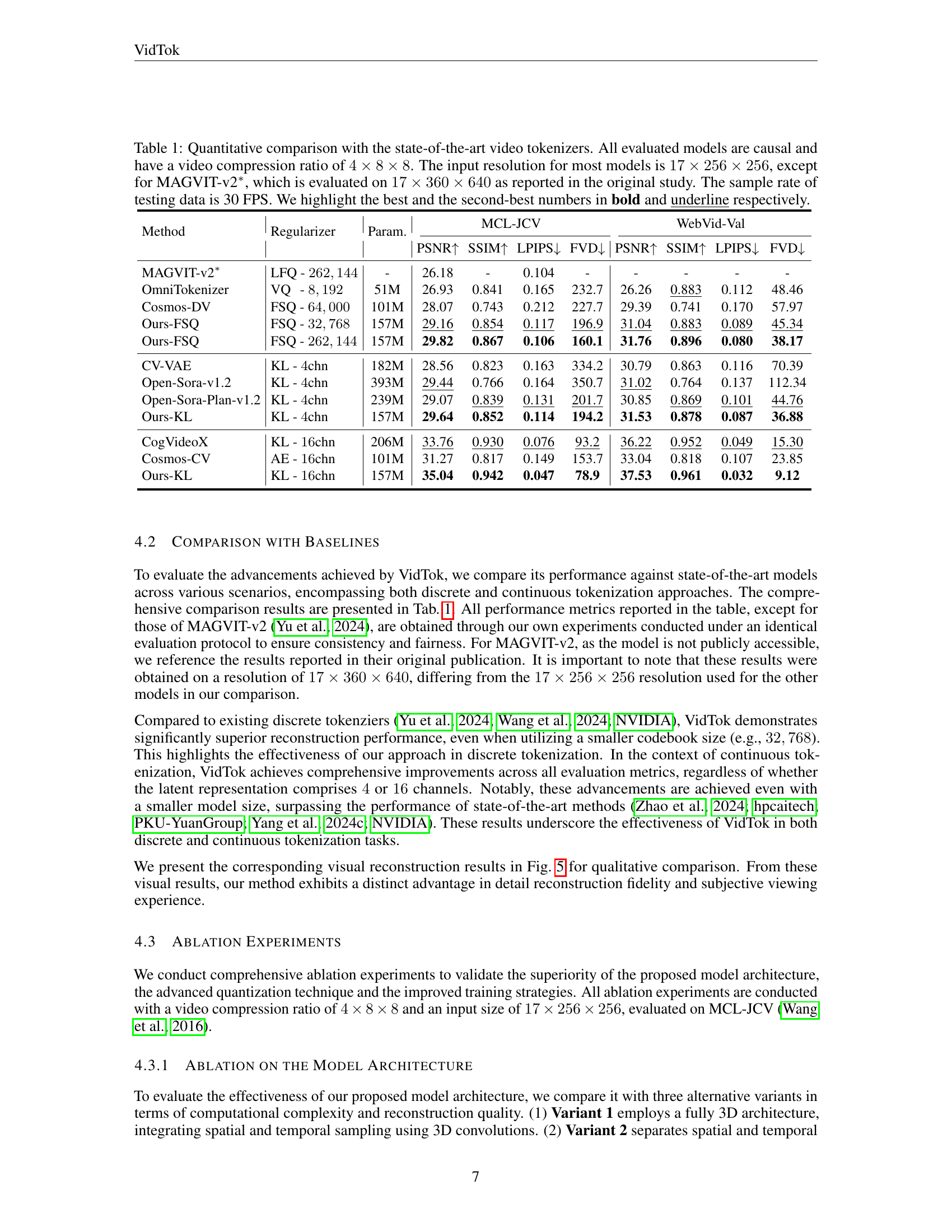
| Method | Regularizer | Param. | MCL-JCV | WebVid-Val | ||||||
|---|---|---|---|---|---|---|---|---|---|---|
| PSNR↑ | SSIM↑ | LPIPS↓ | FVD↓ | PSNR↑ | SSIM↑ | LPIPS↓ | FVD↓ | |||
| MAGVIT-v2∗ | LFQ - 262,144 | - | 26.18 | - | 0.104 | - | - | - | - | - |
| OmniTokenizer | VQ - 8,192 | 51M | 26.93 | 0.841 | 0.165 | 232.7 | 26.26 | 0.883 | 0.112 | 48.46 |
| Cosmos-DV | FSQ - 64,000 | 101M | 28.07 | 0.743 | 0.212 | 227.7 | 29.39 | 0.741 | 0.170 | 57.97 |
| Ours-FSQ | FSQ - 32,768 | 157M | 29.16 | 0.854 | 0.117 | 196.9 | 31.04 | 0.883 | 0.089 | 45.34 |
| Ours-FSQ | FSQ - 262,144 | 157M | 29.82 | 0.867 | 0.106 | 160.1 | 31.76 | 0.896 | 0.080 | 38.17 |
| CV-VAE | KL - 4chn | 182M | 28.56 | 0.823 | 0.163 | 334.2 | 30.79 | 0.863 | 0.116 | 70.39 |
| Open-Sora-v1.2 | KL - 4chn | 393M | 29.44 | 0.766 | 0.164 | 350.7 | 31.02 | 0.764 | 0.137 | 112.34 |
| Open-Sora-Plan-v1.2 | KL - 4chn | 239M | 29.07 | 0.839 | 0.131 | 201.7 | 30.85 | 0.869 | 0.101 | 44.76 |
| Ours-KL | KL - 4chn | 157M | 29.64 | 0.852 | 0.114 | 194.2 | 31.53 | 0.878 | 0.087 | 36.88 |
| CogVideoX | KL - 16chn | 206M | 33.76 | 0.930 | 0.076 | 93.2 | 36.22 | 0.952 | 0.049 | 15.30 |
| Cosmos-CV | AE - 16chn | 101M | 31.27 | 0.817 | 0.149 | 153.7 | 33.04 | 0.818 | 0.107 | 23.85 |
| Ours-KL | KL - 16chn | 157M | 35.04 | 0.942 | 0.047 | 78.9 | 37.53 | 0.961 | 0.032 | 9.12 |
🔼 This table presents a quantitative comparison of VidTok with state-of-the-art causal video tokenizers, using a video compression ratio of 4x8x8. Metrics include PSNR, SSIM, LPIPS, and FVD, evaluated on MCL-JCV and WebVid-Val datasets at 30 FPS. Input resolution is 17x256x256, except for MAGVIT-v2*, which uses 17x360x640 as reported in its original study. Best and second-best results are highlighted.
read the caption
Table 1: Quantitative comparison with the state-of-the-art video tokenizers. All evaluated models are causal and have a video compression ratio of 4×8×84884\times 8\times 84 × 8 × 8. The input resolution for most models is 17×256×2561725625617\times 256\times 25617 × 256 × 256, except for MAGVIT-v2∗, which is evaluated on 17×360×6401736064017\times 360\times 64017 × 360 × 640 as reported in the original study. The sample rate of testing data is 30 FPS. We highlight the best and the second-best numbers in bold and underline respectively.
In-depth insights#
Video Tokenization#
Video tokenization transforms raw video data into compact latent tokens, offering a more efficient representation for video generation and understanding. This approach addresses the inherent redundancy in pixel-level representations, crucial for resource-intensive tasks. Existing image tokenizers fall short when applied to videos due to their inability to capture temporal dynamics and consistency. VidTok introduces novel solutions to overcome these limitations. Its architecture decouples spatial and temporal sampling, utilizing 2D convolutions for spatial processing and an AlphaBlender for temporal processing, thereby reducing computational demands without sacrificing quality. FSQ addresses training instability and codebook collapse commonly associated with traditional VQ methods, improving efficiency in discrete tokenization. Furthermore, a two-stage training strategy, coupled with reduced frame rate training data, enhances motion dynamic representation and speeds up training, making VidTok a versatile, efficient, and effective video tokenizer.
VidTok Advancements#
VidTok introduces key advancements in video tokenization. Its hybrid architecture, combining 2D and 3D convolutions, balances efficiency and performance. Using Finite Scalar Quantization (FSQ) improves discrete tokenization by directly optimizing an implicit codebook, enhancing stability and utilization compared to traditional Vector Quantization (VQ). A two-stage training process, starting with lower resolution and fine-tuning on higher resolution, cuts computational costs significantly. Training with reduced frame rates further improves motion dynamics representation. These combined advancements position VidTok as a versatile, high-performing video tokenizer for various applications.
FSQ for Stability#
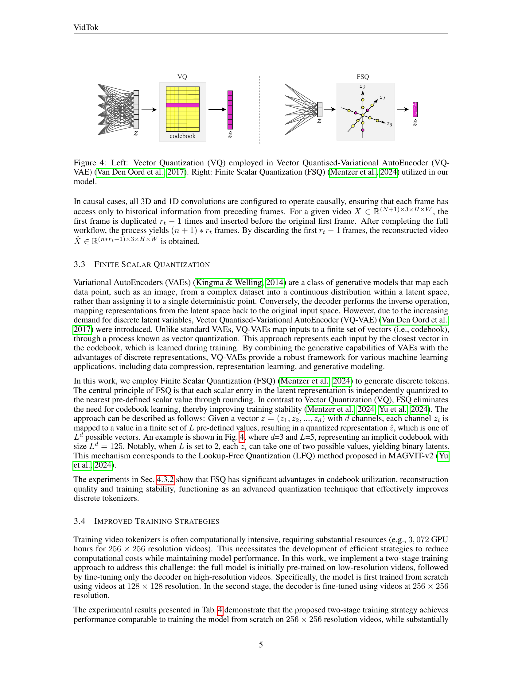
FSQ (Finite Scalar Quantization) offers a compelling alternative to traditional Vector Quantization (VQ) methods for video tokenization by directly quantizing latent representations to pre-defined scalar values. This eliminates the need for learning a codebook, a process often plagued by instability and codebook collapse. By simplifying the quantization mechanism, FSQ enhances training stability and improves codebook utilization, leading to higher fidelity reconstructions. This stability is crucial for generating high-quality video tokens, enabling a more robust foundation for downstream tasks such as video generation and understanding. Furthermore, the implicit nature of FSQ’s codebook avoids explicit storage, making the approach more memory-efficient. These advantages position FSQ as a highly promising technique for enhancing video tokenization and facilitating advancements in video-related research.
Two-Stage Training#
Two-stage training significantly reduces computational costs while maintaining performance. Initially, the full model is pre-trained on low-resolution videos. Subsequently, only the decoder is fine-tuned on high-resolution videos. This approach cuts training time in half compared to training solely on high-resolution videos. Furthermore, this strategy facilitates adaptation to new domains without retraining the entire model, preserving compatibility with the initial latent space. The fixed encoder enables latent models trained in the shared space to be reused across resolutions and domains. This modular training approach allows for efficient resource utilization and scalability.
Open-Source VidTok#
VidTok’s open-source nature democratizes cutting-edge video technology. Researchers and developers gain access to a high-performing, versatile tokenizer, fostering innovation. Its availability lowers the barrier to exploring video generation, understanding, and advanced editing techniques. This accelerates research, leading to breakthroughs in areas like video diffusion models. By open-sourcing VidTok, wider community contributions and scrutiny can enhance robustness and capabilities, impacting applications across multiple domains.
More visual insights#
More on figures

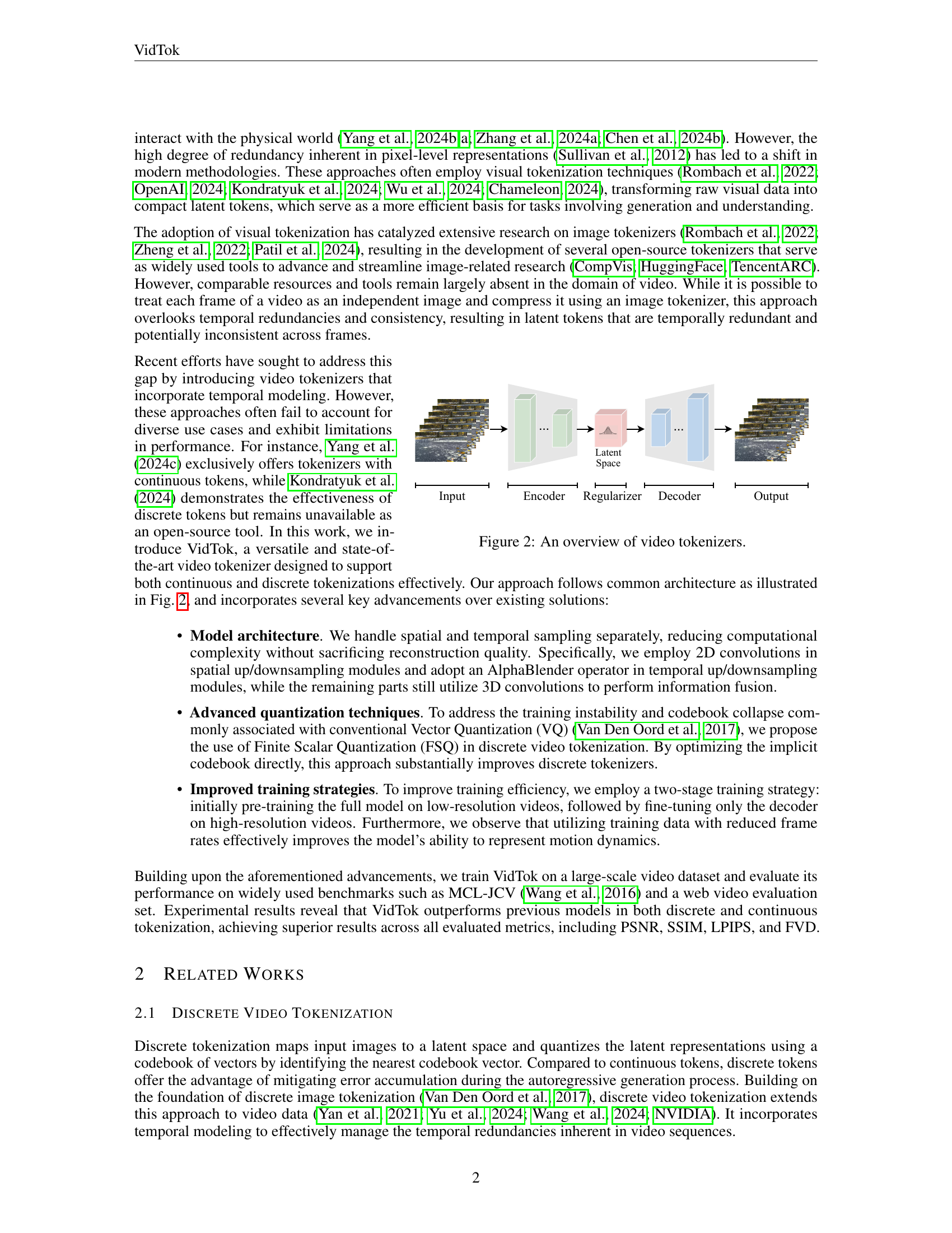
🔼 This figure presents a high-level overview of the typical architecture of a video tokenizer. The diagram illustrates the key components and the flow of information during the tokenization and reconstruction process. A video input is first fed into an encoder, which compresses the video into a compact representation within a latent space. Within this latent space, a regularizer is often applied to enforce certain properties or constraints, such as sparsity or smoothness. Finally, a decoder takes the regularized latent representation and reconstructs the original video. Depending on the specific model, the latent space can be either continuous or discrete, and the architecture may operate in a causal or non-causal manner.
read the caption
Figure 2: An overview of video tokenizers.

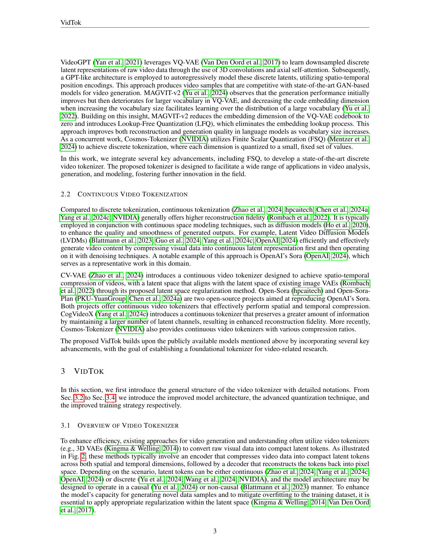
🔼 The figure presents the architecture of the video tokenizer, VidTok. It visually illustrates the flow of data through the model, highlighting the components responsible for temporal and spatial compression and decompression. The model takes a video input of size T×H×W (Time × Height × Width) and compresses it into a latent representation of smaller dimensions using an encoder with 2D convolutions and an AlphaBlender operator. It then reconstructs the original video from the latent representation using a decoder with a similar structure, including 2D convolutions and AlphaBlender. In the context of causal video processing, additional considerations are introduced. The first frame is processed differently to allow the model to function for single images as well. The diagram also depicts the specific modules used for temporal upsampling and downsampling. The improved model architecture uses a combination of 2D and 3D convolutional layers to reduce computational demands without compromising performance.
read the caption
Figure 3: The improved model architecture. In the context of a causal setting, consider an input with dimensions T×H×W=17×256×256𝑇𝐻𝑊17256256T\times H\times W=17\times 256\times 256italic_T × italic_H × italic_W = 17 × 256 × 256. Assuming a temporal compression factor of 4444 and a spatial compression factor of 8888, the intermediate latent representation is reduced to dimensions T×H×W=5×32×32𝑇𝐻𝑊53232T\times H\times W=5\times 32\times 32italic_T × italic_H × italic_W = 5 × 32 × 32.

🔼 The figure provides a visual comparison of two quantization methods used in the proposed video tokenizer model, VidTok. Vector Quantization (VQ), shown on the left, maps latent vectors to entries in a learned codebook. This is the method used in VQ-VAE (Vector Quantised-Variational AutoEncoder). Finite Scalar Quantization (FSQ), shown on the right, directly quantizes each scalar value in the latent space to predefined discrete levels and does not require learning a codebook. VidTok uses FSQ. FSQ enhances training stability and improves codebook utilization.
read the caption
Figure 4: Left: Vector Quantization (VQ) employed in Vector Quantised-Variational AutoEncoder (VQ-VAE) (Van Den Oord et al., 2017). Right: Finite Scalar Quantization (FSQ) (Mentzer et al., 2024) utilized in our model.

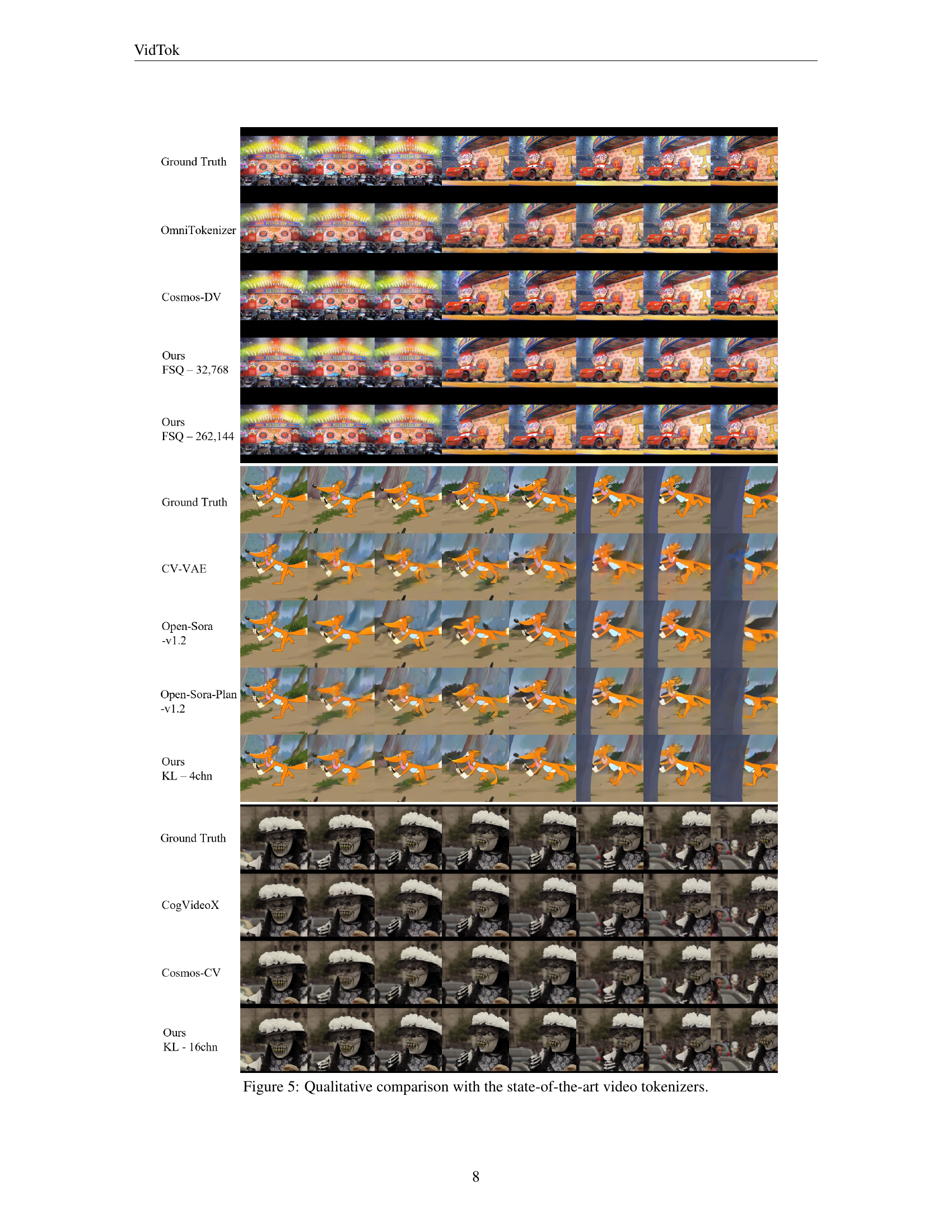
🔼 Qualitative comparison of VidTok with state-of-the-art video tokenizers, showcasing the effectiveness of VidTok in reconstructing video frames with high fidelity. The comparison includes various state-of-the-art models such as OmniTokenizer, Cosmos-DV, CV-VAE, Open-Sora-v1.2, Open-Sora-Plan-v1.2, and CogVideoX, across a range of video content. The reconstructed frames by each model are juxtaposed with the original frames, allowing a clear assessment of their performance.
read the caption
Figure 5: Qualitative comparison with the state-of-the-art video tokenizers.

🔼 This figure shows the impact of using different frame rates for the training data on the performance of a video tokenizer model. The top row displays the ground truth frames. The middle row shows the reconstructed frames when the model was trained with data at 8 frames per second (FPS). The bottom row shows the results when trained with data at 3 FPS. The comparison suggests that training with a lower frame rate (3 FPS) leads to better capturing of motion dynamics, resulting in improved reconstruction, especially noticeable in the fox’s legs and tail. This observation implies that a lower frame rate during training might encourage the model to focus more on the overall motion flow rather than fine-grained details within individual frames.
read the caption
Figure 6: The influence of different sample rates on model performance during training. The second row presents the test results obtained using training data with a sample rate of 8 FPS, while the third row shows the test results using training data with a sample rate of 3 FPS. The results demonstrate that employing training data with reduced frame rates enhances the model’s capacity to effectively capture motion dynamics.
More on tables
| Method | Param. | FLOPs | PSNR↑ | SSIM↑ | LPIPS↓ | FVD↓ |
|---|---|---|---|---|---|---|
| Variant 1 | 245M | 16.98 T | 29.39 | 0.847 | 0.117 | 176.9 |
| Variant 2 | 142M | 7.17 T | 29.36 | 0.846 | 0.119 | 185.7 |
| Variant 3 | 126M | 10.18 T | 29.26 | 0.846 | 0.120 | 200.6 |
| Ours | 157M | 10.35 T | 29.64 | 0.852 | 0.114 | 194.2 |
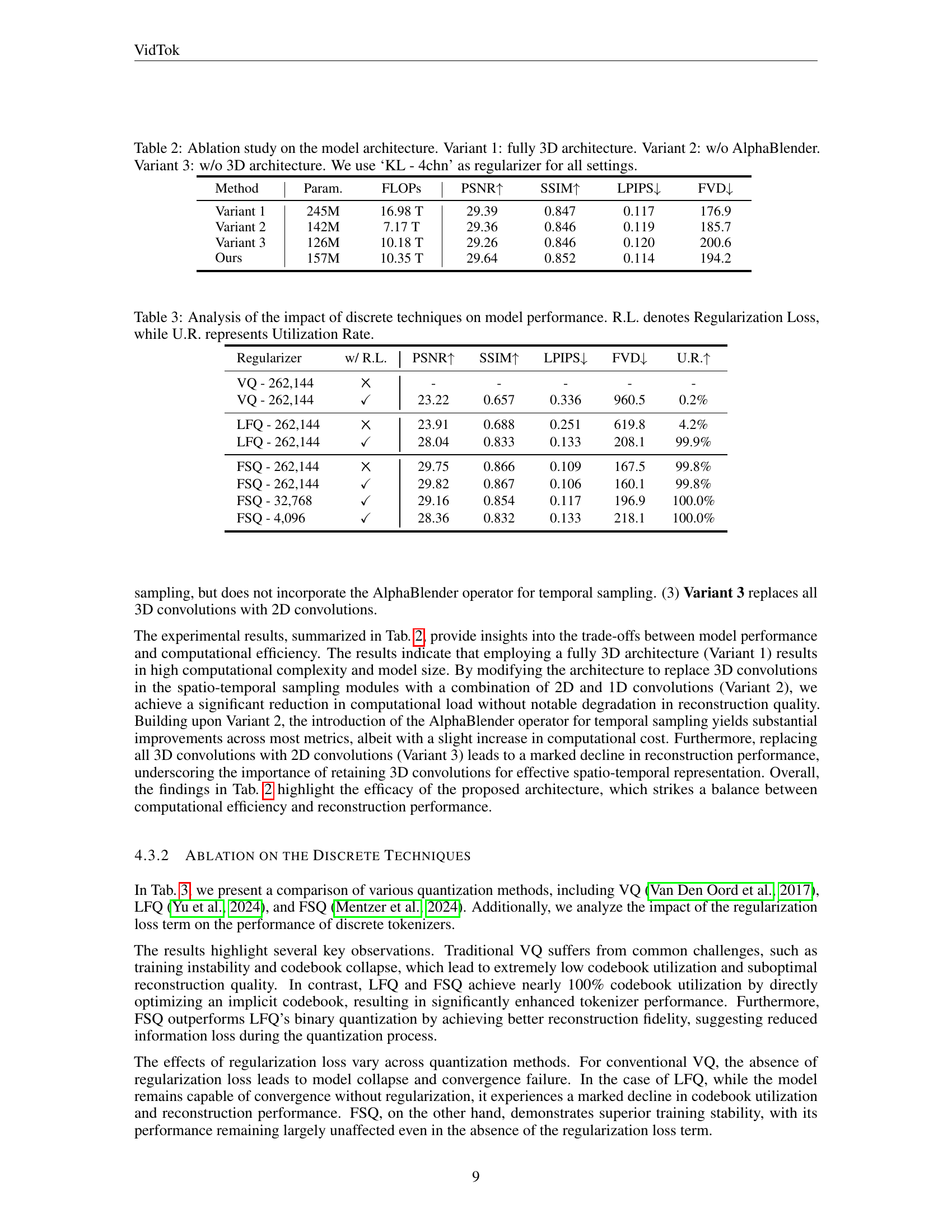
🔼 This table presents an ablation study on the model architecture for video tokenization, comparing the performance of four different architectures. All models are trained using ‘KL - 4chn’ as regularizer. Variant 1 uses a fully 3D architecture for spatial and temporal sampling. Variant 2 separates spatial and temporal sampling using 2D and 1D convolutions but without AlphaBlender. Variant 3 replaces all 3D convolutions with 2D convolutions. The proposed Ours model utilizes a combination of 2D and 1D convolutions with the AlphaBlender operator for temporal upsampling and downsampling, while other parts leverage 3D convolutions for information fusion. The table compares the number of parameters (Param.), FLOPS (floating point operations per second), Peak Signal-to-Noise Ratio (PSNR), Structural Similarity Index Measure (SSIM), Learned Perceptual Image Patch Similarity (LPIPS), and Fréchet Video Distance (FVD). The results demonstrate that the proposed architecture strikes a balance between computational efficiency and reconstruction performance.
read the caption
Table 2: Ablation study on the model architecture. Variant 1: fully 3D architecture. Variant 2: w/o AlphaBlender. Variant 3: w/o 3D architecture. We use ‘KL - 4chn’ as regularizer for all settings.
| Regularizer | w/ R.L. | PSNR↑ | SSIM↑ | LPIPS↓ | FVD↓ | U.R.↑ |
|---|---|---|---|---|---|---|
| VQ - 262,144 | \usym2613 | - | - | - | - | - |
| VQ - 262,144 | ✓ | 23.22 | 0.657 | 0.336 | 960.5 | 0.2% |
| LFQ - 262,144 | \usym2613 | 23.91 | 0.688 | 0.251 | 619.8 | 4.2% |
| LFQ - 262,144 | ✓ | 28.04 | 0.833 | 0.133 | 208.1 | 99.9% |
| FSQ - 262,144 | \usym2613 | 29.75 | 0.866 | 0.109 | 167.5 | 99.8% |
| FSQ - 262,144 | ✓ | 29.82 | 0.867 | 0.106 | 160.1 | 99.8% |
| FSQ - 32,768 | ✓ | 29.16 | 0.854 | 0.117 | 196.9 | 100.0% |
| FSQ - 4,096 | ✓ | 28.36 | 0.832 | 0.133 | 218.1 | 100.0% |
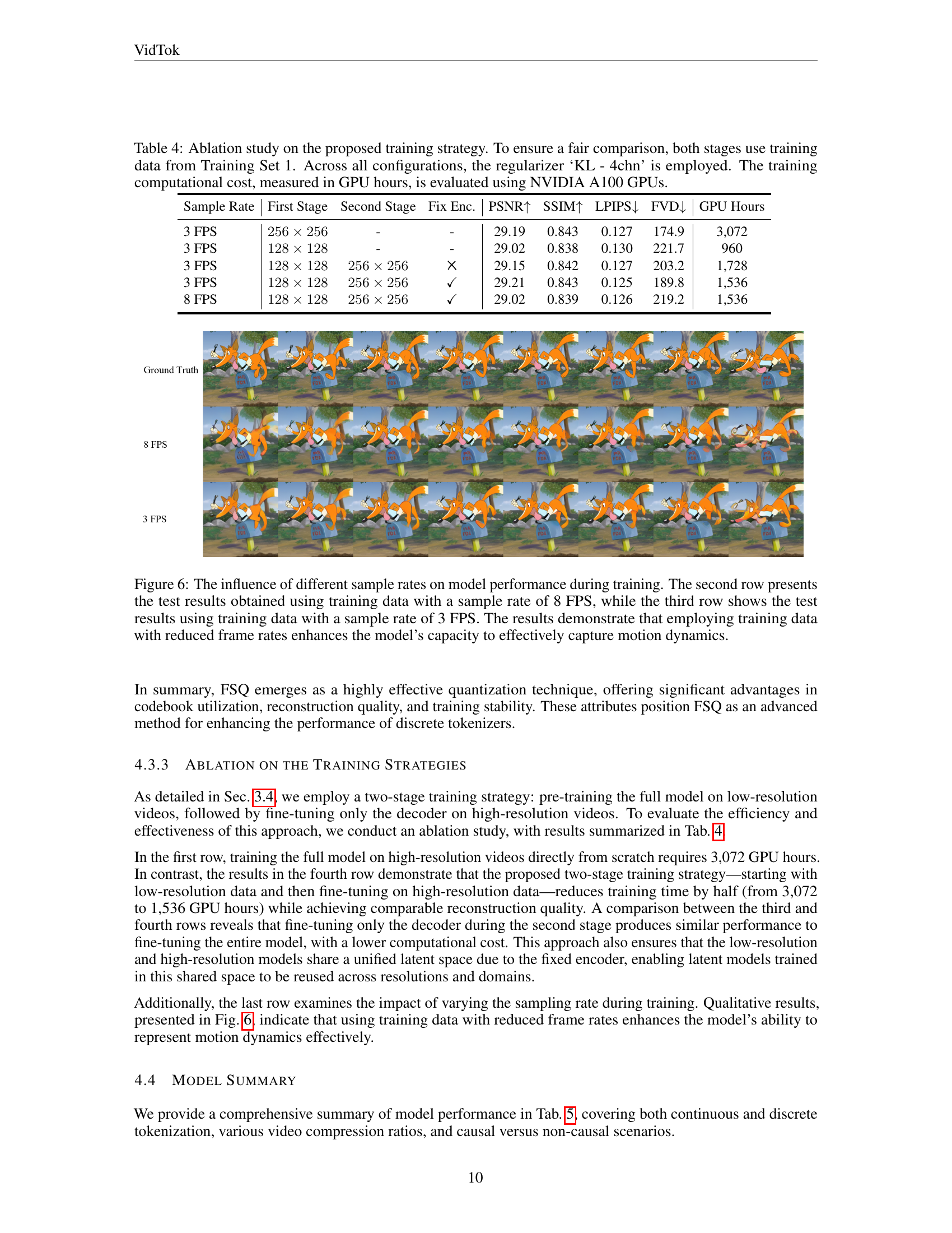
🔼 This table shows the ablation study conducted on discrete techniques including VQ, LFQ, and FSQ, demonstrating FSQ’s significant advantages over existing discrete tokenization techniques in terms of codebook utilization, reconstruction quality, and training stability. The presence or absence of regularization loss is also considered during the ablation analysis.
read the caption
Table 3: Analysis of the impact of discrete techniques on model performance. R.L. denotes Regularization Loss, while U.R. represents Utilization Rate.
| Sample Rate | First Stage | Second Stage | Fix Enc. | PSNR↑ | SSIM↑ | LPIPS↓ | FVD↓ | GPU Hours |
|---|---|---|---|---|---|---|---|---|
| 3 FPS | 256x256 | - | - | 29.19 | 0.843 | 0.127 | 174.9 | 3,072 |
| 3 FPS | 128x128 | - | - | 29.02 | 0.838 | 0.130 | 221.7 | 960 |
| 3 FPS | 128x128 | 256x256 | \usym2613 | 29.15 | 0.842 | 0.127 | 203.2 | 1,728 |
| 3 FPS | 128x128 | 256x256 | ✓ | 29.21 | 0.843 | 0.125 | 189.8 | 1,536 |
| 8 FPS | 128x128 | 256x256 | ✓ | 29.02 | 0.839 | 0.126 | 219.2 | 1,536 |
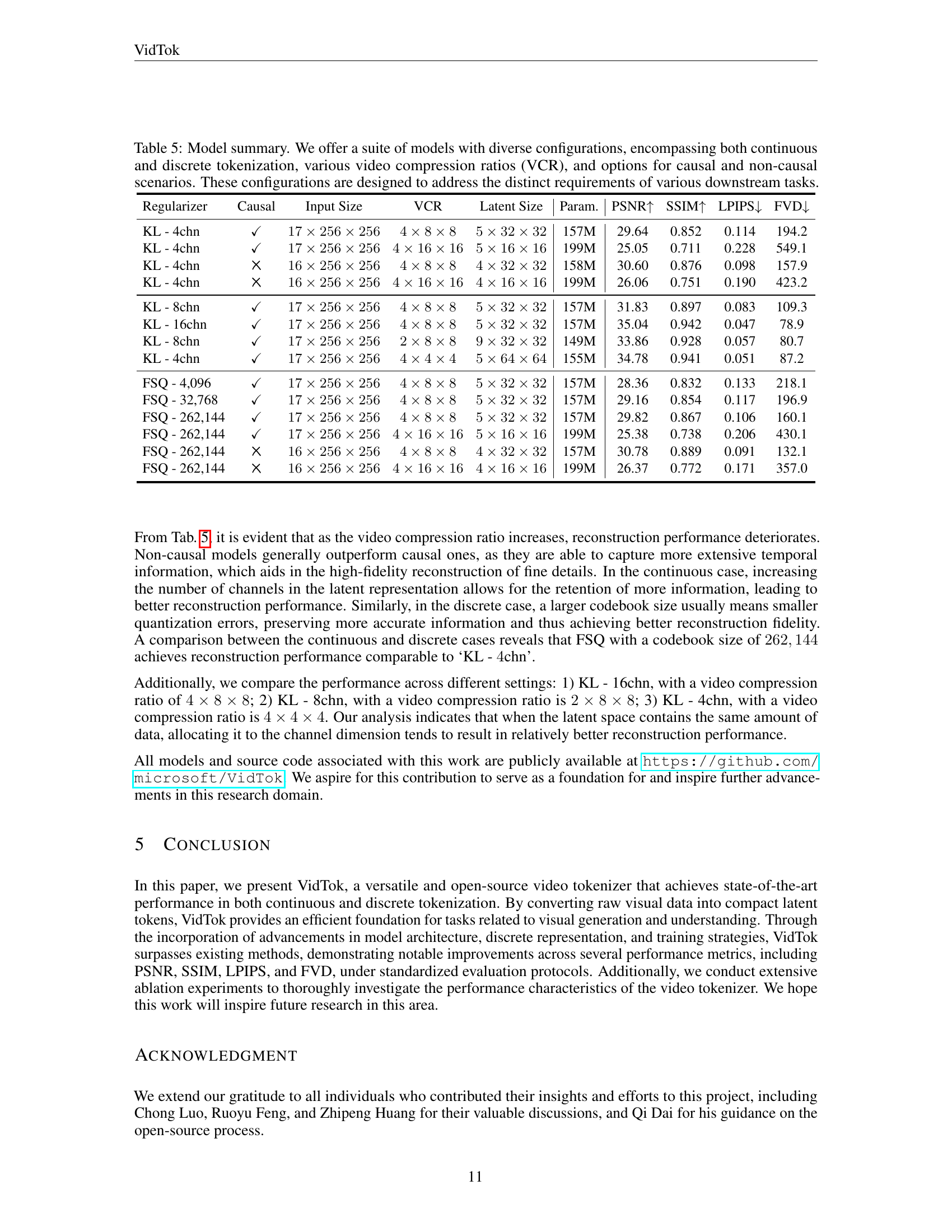
🔼 This table presents the ablation study on the two-stage training strategy proposed in the paper. The first stage involves training the full model on low-resolution videos (128x128), while the second stage involves fine-tuning only the decoder on high-resolution videos (256x256). The table compares different training settings, including single-stage training on high-resolution videos, two-stage training with or without fixed encoder, and varying sample rates. The results demonstrate that the two-stage training strategy with a fixed encoder achieves similar performance to single-stage training on high resolution but at roughly half the training time.
read the caption
Table 4: Ablation study on the proposed training strategy. To ensure a fair comparison, both stages use training data from Training Set 1. Across all configurations, the regularizer ‘KL - 4chn’ is employed. The training computational cost, measured in GPU hours, is evaluated using NVIDIA A100 GPUs.
| Regularizer | Causal | Input Size | VCR | Latent Size | Param. | PSNR↑ | SSIM↑ | LPIPS↓ | FVD↓ |
|---|---|---|---|---|---|---|---|---|---|
| KL - 4chn | ✓ | 17×256×256 | 4×8×8 | 5×32×32 | 157M | 29.64 | 0.852 | 0.114 | 194.2 |
| KL - 4chn | ✓ | 17×256×256 | 4×16×16 | 5×16×16 | 199M | 25.05 | 0.711 | 0.228 | 549.1 |
| KL - 4chn | \usym2613 | 16×256×256 | 4×8×8 | 4×32×32 | 158M | 30.60 | 0.876 | 0.098 | 157.9 |
| KL - 4chn | \usym2613 | 16×256×256 | 4×16×16 | 4×16×16 | 199M | 26.06 | 0.751 | 0.190 | 423.2 |
| KL - 8chn | ✓ | 17×256×256 | 4×8×8 | 5×32×32 | 157M | 31.83 | 0.897 | 0.083 | 109.3 |
| KL - 16chn | ✓ | 17×256×256 | 4×8×8 | 5×32×32 | 157M | 35.04 | 0.942 | 0.047 | 78.9 |
| KL - 8chn | ✓ | 17×256×256 | 2×8×8 | 9×32×32 | 149M | 33.86 | 0.928 | 0.057 | 80.7 |
| KL - 4chn | ✓ | 17×256×256 | 4×4×4 | 5×64×64 | 155M | 34.78 | 0.941 | 0.051 | 87.2 |
| FSQ - 4,096 | ✓ | 17×256×256 | 4×8×8 | 5×32×32 | 157M | 28.36 | 0.832 | 0.133 | 218.1 |
| FSQ - 32,768 | ✓ | 17×256×256 | 4×8×8 | 5×32×32 | 157M | 29.16 | 0.854 | 0.117 | 196.9 |
| FSQ - 262,144 | ✓ | 17×256×256 | 4×8×8 | 5×32×32 | 157M | 29.82 | 0.867 | 0.106 | 160.1 |
| FSQ - 262,144 | ✓ | 17×256×256 | 4×16×16 | 5×16×16 | 199M | 25.38 | 0.738 | 0.206 | 430.1 |
| FSQ - 262,144 | \usym2613 | 16×256×256 | 4×8×8 | 4×32×32 | 157M | 30.78 | 0.889 | 0.091 | 132.1 |
| FSQ - 262,144 | \usym2613 | 16×256×256 | 4×16×16 | 4×16×16 | 199M | 26.37 | 0.772 | 0.171 | 357.0 |
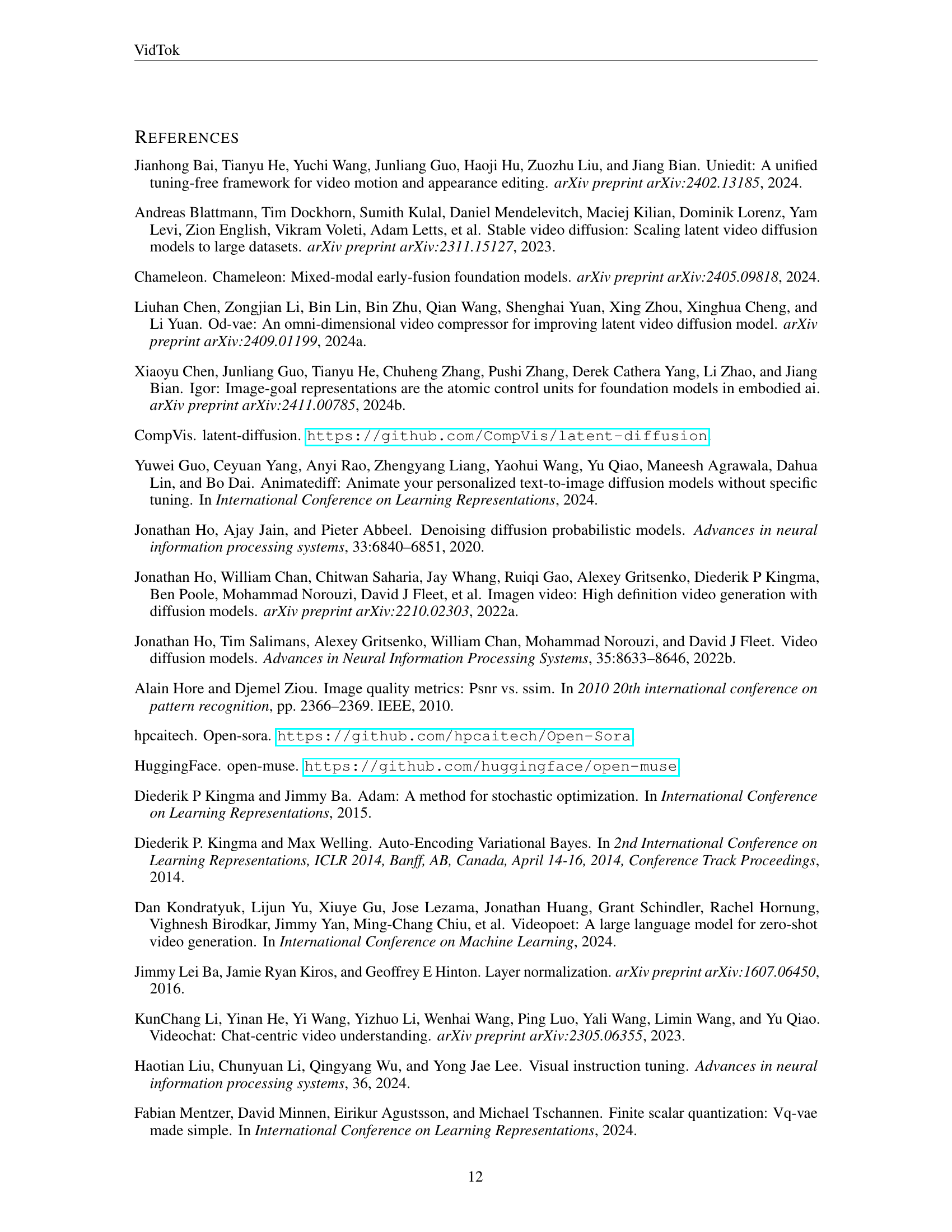
🔼 This table provides a comprehensive overview of the different VidTok model configurations. It shows variations based on continuous vs. discrete tokenization, different video compression ratios (how much the video is compressed), whether the model is causal (processes information sequentially) or non-causal (processes information in any order), the latent space size, model parameters, and performance metrics (PSNR, SSIM, LPIPS, and FVD). This variety allows users to select the best model for their specific needs, whether it’s high-fidelity reconstruction or efficient compression.
read the caption
Table 5: Model summary. We offer a suite of models with diverse configurations, encompassing both continuous and discrete tokenization, various video compression ratios (VCR), and options for causal and non-causal scenarios. These configurations are designed to address the distinct requirements of various downstream tasks.
Full paper#
