↗ arXiv ↗ Hugging Face ↗ Papers with Code
TL;DR#
Large language models (LLMs) have achieved remarkable success, but recent research indicates their deep layers are often underutilized. Pre-LN, a common normalization technique in LLMs, leads to diminishing gradients in deeper layers, hindering their learning. This inefficiency wastes computational resources and limits potential model performance. While Post-LN maintains strong deep layer gradients, it suffers from vanishing gradients in early layers. Existing research often frames this inefficiency as a compression opportunity, overlooking the potential of unlocking these layers’ full capacity.
This paper introduces Mix-LN, a novel normalization technique that combines Pre-LN and Post-LN. Mix-LN applies Post-LN in initial layers and Pre-LN in later layers. This creates more uniform gradient norms, allowing both shallow and deep layers to contribute effectively. Experiments across various LLM sizes show that Mix-LN consistently outperforms Pre-LN and Post-LN. It achieves better pre-training results, more effective supervised fine-tuning, and enhanced reinforcement learning from human feedback (RLHF). The findings underscore the importance of high-quality deep layers for powerful LLMs, offering a promising way to improve performance without increasing model size.
Key Takeaways#
Why does it matter?#
Mix-LN’s impact is significant for LLM training. It addresses a critical training shortfall by improving deep layer utilization. This leads to enhanced model capacity and efficiency without architectural changes. This opens new research avenues into normalization techniques, inspiring further exploration of methods for maximizing network potential. The demonstration of improved fine-tuning and RLHF performance with Mix-LN highlights its practical relevance for LLM deployment, particularly in resource-intensive scenarios.
Visual Insights#

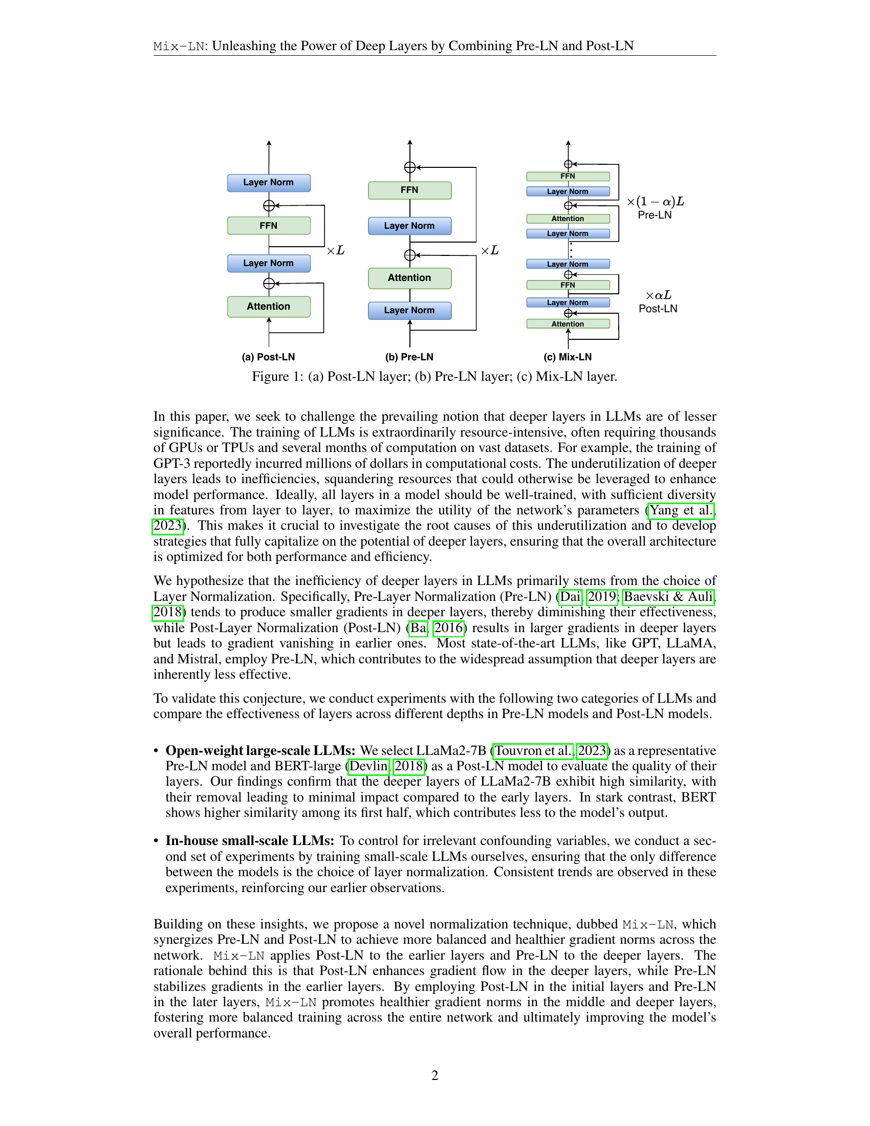
🔼 This figure visually represents the architecture of three different layer normalization techniques within the context of transformer layers: Post-LN, Pre-LN and Mix-LN. Post-LN applies layer normalization after the residual connection adding the output of the attention or FFN block to the input of the block, Pre-LN applies it before the residual connection and Mix-LN combines Post-LN and Pre-LN within the same model. Mix-LN applies Post-LN to the earlier layers and Pre-LN to the deeper layers, in order to ensure more uniform gradients across layers. In the figure, ‘x’ represents the input to the layer, ‘Layer Norm’ is the layer normalization operation, and both ‘Attention’ and ‘FFN’ represent multi-head attention and feed-forward network blocks, respectively.
read the caption
Figure 1: (a) Post-LN layer; (b) Pre-LN layer; (c) Mix-LN layer.
| LLaMA-71M | LLaMA-130M | LLaMA-250M | LLaMA-1B | |
|---|---|---|---|---|
| Training Tokens | 1.1B | 2.2B | 3.9B | 5B |
| Post-LN | 35.18 | 26.95 | 1409.09 | 1411.54 |
| DeepNorm | 34.87 | 27.17 | 22.77 | 1410.94 |
| Pre-LN | 34.77 | 26.78 | 21.92 | 18.65 |
| Mix-LN | 33.12 | 26.07 | 21.39 | 18.18 |
🔼 This table presents a comparison of perplexity scores achieved by different normalization methods (Post-LN, DeepNorm, Pre-LN, and Mix-LN) when applied to various LLaMA models of different sizes (71M, 130M, 250M, and 1B parameters). The training was conducted with varying numbers of training tokens depending on the model size. Lower perplexity scores indicate better performance.
read the caption
Table 1: Perplexity (↓↓\downarrow↓) comparison of various normalization methods across various LLaMA sizes.
In-depth insights#
Pre-LN Inadequacy#
Pre-LN’s limitations stem from its impact on gradient flow in deep networks. While it mitigates vanishing gradients in initial layers, it inadvertently reduces gradients in deeper layers. This creates an imbalance, where earlier layers dominate learning while deeper layers contribute less. Consequently, the full potential of the network remains untapped, hindering performance. This issue is not merely a compression opportunity, but a training deficiency that needs addressing. The deeper layers’ underutilization in Pre-LN models signifies a crucial area for improvement in training deep networks. Mix-LN addresses this by combining Pre-LN and Post-LN to improve gradient flow.
Mix-LN Synergy#
Mix-LN synergistically combines the strengths of Pre-LN and Post-LN. Pre-LN’s stable early-layer gradients and Post-LN’s robust deep-layer gradients are leveraged for enhanced overall performance. This synergy addresses the ineffectiveness of deeper layers in LLMs trained with Pre-LN by mitigating gradient degradation. The strategic application of Post-LN to initial layers and Pre-LN to deeper layers facilitates balanced gradient flow throughout the model. Mix-LN further stabilizes training dynamics associated with Post-LN, thus enabling efficient utilization of all model layers. Consequently, this method fosters improved feature diversity and richness across layers, leading to more robust and effective LLM training. This synergy contributes to more nuanced and generalized predictions, notably improving performance across various tasks and model sizes.
Gradient Balancing#
Gradient balancing is crucial for effective deep learning model training. It addresses issues like vanishing or exploding gradients, especially in deep networks. Techniques like Mix-LN combine the strengths of pre- and post-layer normalization to ensure more uniform gradient norms across layers. This balances training across all layers, preventing underutilization of deeper layers and improving overall model capacity and performance. It helps avoid training instabilities associated with some normalization methods. Improved gradient flow allows all layers to contribute more effectively, especially during fine-tuning and reinforcement learning stages, impacting areas like natural language processing and computer vision.
LLM Enhancement#
Mix-LN significantly enhances LLMs by optimizing deep layer training. Pre-LN’s gradient limitations hinder deep layer effectiveness, while Post-LN causes gradient vanishing in early layers. Mix-LN strategically combines both, applying Post-LN initially and Pre-LN later. This balances gradient flow, maximizing deep layer contribution and overall model capacity. Experimental results across various model sizes and tasks demonstrate consistent perplexity reduction and performance gains in fine-tuning and RLHF, confirming Mix-LN’s effectiveness in unlocking LLM potential.
Normalization Limits#
Normalization, while crucial in LLMs, faces limitations primarily due to gradient behavior. Pre-LN excels in early layers, mitigating vanishing gradients but hampering deeper layer effectiveness. Post-LN suffers from training instability, hindering convergence in larger models. These issues highlight a trade-off, where each technique’s strength becomes its weakness. Mix-LN leverages this dynamic, using Post-LN for initial layers to address early vanishing gradients, and Pre-LN for deeper layers to optimize gradient flow, allowing each technique to supplement the other.
More visual insights#
More on figures

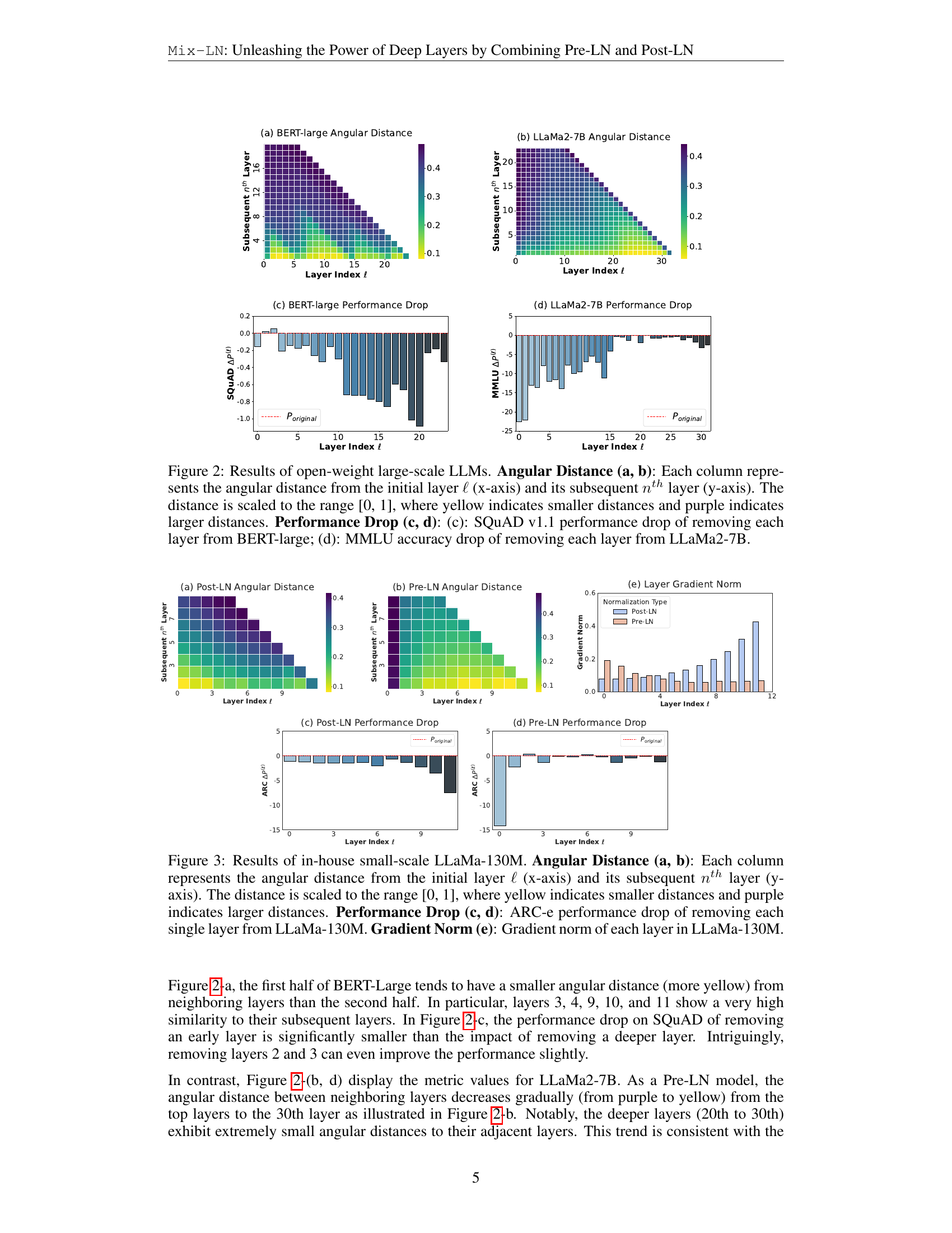
🔼 This figure presents an analysis of two large language models (LLMs), BERT-large and LLaMa2-7B, using two metrics: Angular Distance and Performance Drop. Angular Distance measures the similarity between the activations of a layer and a subsequent layer. A smaller distance (yellow) implies greater similarity and potentially redundancy. Performance drop measures the decrease in model performance when a specific layer is removed. A larger drop indicates the layer is more important. Subfigures (a) and (c) show these metrics for BERT-large (a Post-LN model), while (b) and (d) show the same for LLaMa2-7B (a Pre-LN model). The results demonstrate the differing behavior of layer effectiveness between these normalization methods.
read the caption
Figure 2: Results of open-weight large-scale LLMs. Angular Distance (a, b): Each column represents the angular distance from the initial layer ℓℓ\ellroman_ℓ (x-axis) and its subsequent nthsuperscript𝑛𝑡ℎn^{th}italic_n start_POSTSUPERSCRIPT italic_t italic_h end_POSTSUPERSCRIPT layer (y-axis). The distance is scaled to the range [0, 1], where yellow indicates smaller distances and purple indicates larger distances. Performance Drop (c, d): (c): SQuAD v1.1 performance drop of removing each layer from BERT-large; (d): MMLU accuracy drop of removing each layer from LLaMa2-7B.

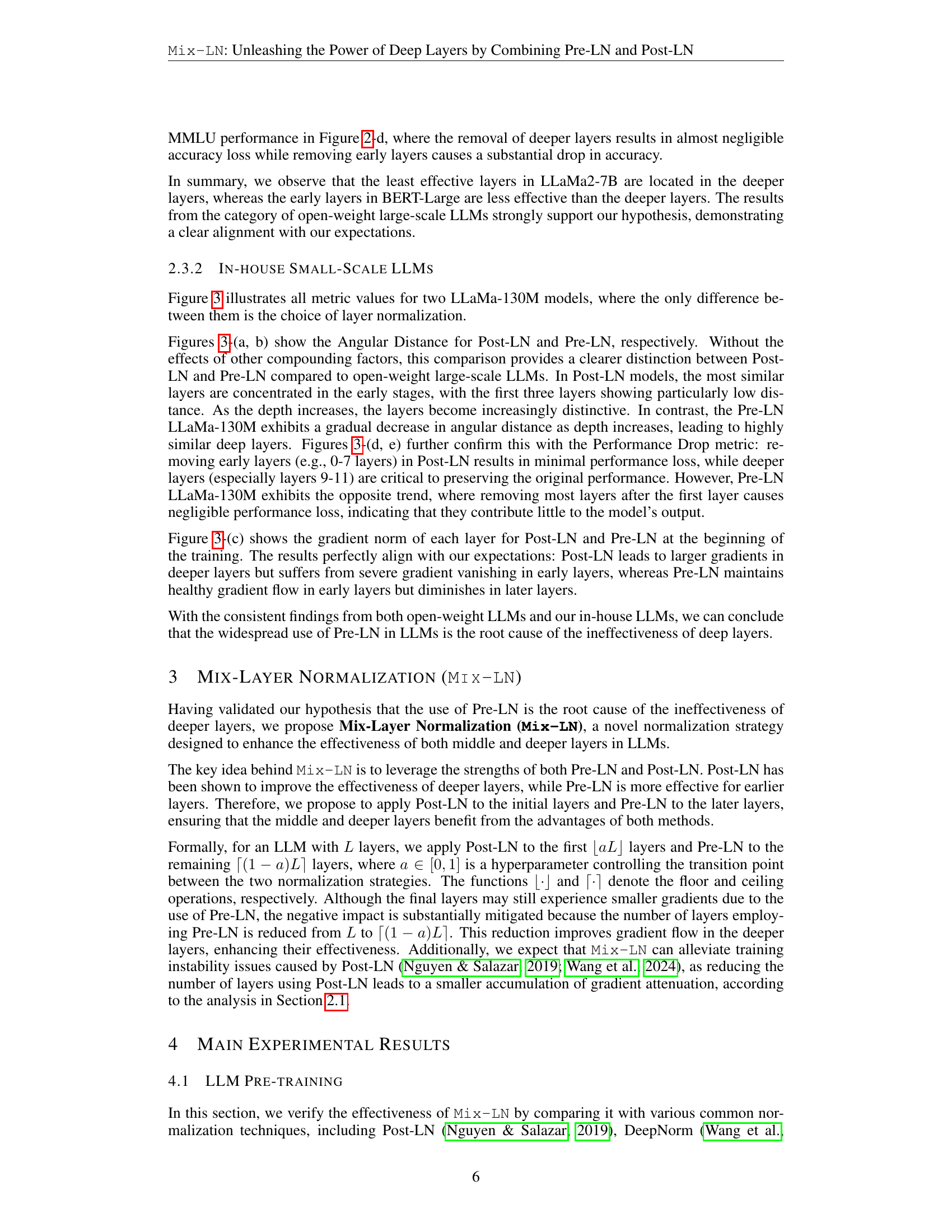
🔼 This figure presents an analysis of in-house trained small-scale LLaMa-130M models, comparing the effectiveness of different normalization methods (Pre-LN, Post-LN, and Mix-LN). Subfigures (a) and (b) visualize the angular distance between layer representations, demonstrating how layer similarity changes with depth in different normalization schemes. Yellow indicates high similarity, purple indicates low similarity. Subfigures (c) and (d) show the performance drop (ARC-e score) resulting from removing individual layers, indicating each layer’s importance. Subfigure (e) displays the gradient norm of each layer for both Post-LN and Pre-LN at the beginning of training, illustrating the impact of normalization on gradient flow.
read the caption
Figure 3: Results of in-house small-scale LLaMa-130M. Angular Distance (a, b): Each column represents the angular distance from the initial layer ℓℓ\ellroman_ℓ (x-axis) and its subsequent nthsuperscript𝑛𝑡ℎn^{th}italic_n start_POSTSUPERSCRIPT italic_t italic_h end_POSTSUPERSCRIPT layer (y-axis). The distance is scaled to the range [0, 1], where yellow indicates smaller distances and purple indicates larger distances. Performance Drop (c, d): ARC-e performance drop of removing each single layer from LLaMa-130M. Gradient Norm (e): Gradient norm of each layer in LLaMa-130M.
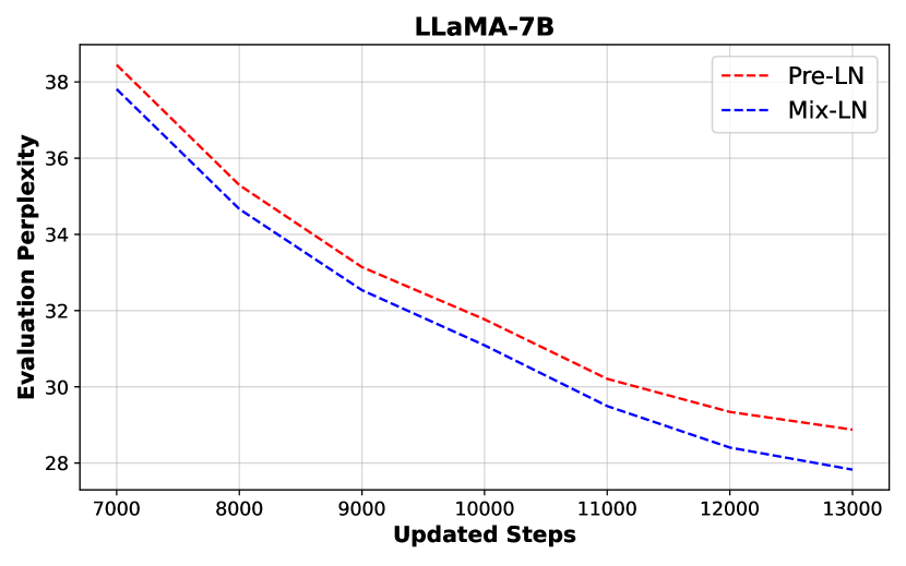
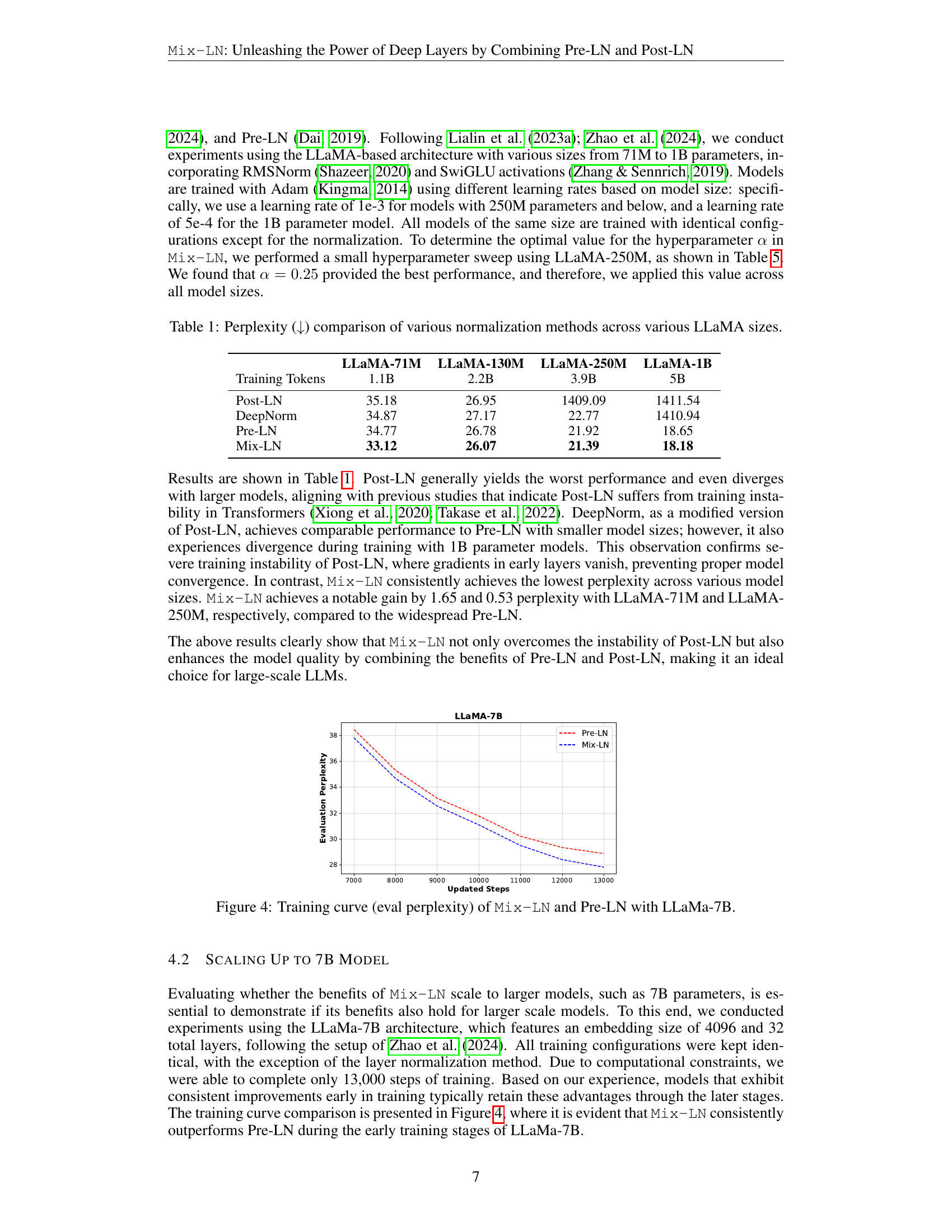
🔼 This figure presents the training curves of LLaMa-7B models using two different layer normalization methods: Mix-LN (proposed method) and the standard Pre-LN. The y-axis represents the evaluation perplexity (lower is better), and the x-axis represents the number of training steps. The plot visually demonstrates that Mix-LN consistently achieves lower perplexity than Pre-LN throughout the training process, suggesting its effectiveness in improving the model’s performance.
read the caption
Figure 4: Training curve (eval perplexity) of Mix-LN and Pre-LN with LLaMa-7B.

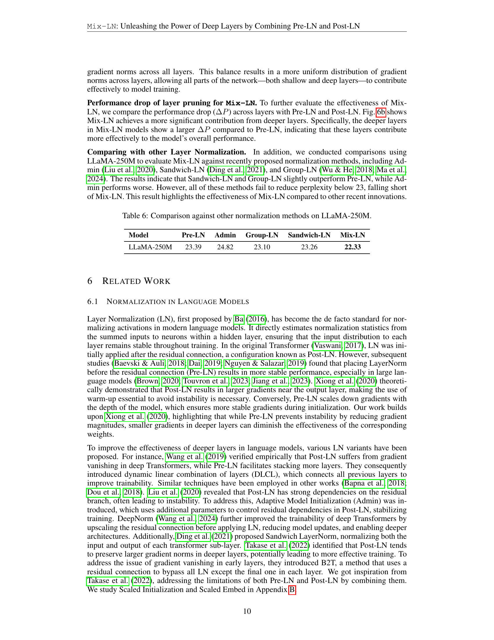
🔼 This figure visualizes the angular distance between the hidden states of different layers in the LLaMA-130M model, comparing Pre-LN, Post-LN, and Mix-LN normalization methods. Each cell (ℓ,n)(ℓ,n)(’ell’, ’n’) in a heatmap represents the angular distance between the input to layer ℓℓ’ell’ and the input to layer ℓ+nℓ+n’ell’ + ’n’. A smaller distance (yellow) indicates higher similarity between layer representations, while a larger distance (purple) suggests greater dissimilarity. Mix-LN tends to produce larger angular distances (more dissimilarity), particularly in the deeper layers, than the other methods, while Post-LN shows high similarity (smaller angular distances) mostly in the earlier layers. This observation illustrates how Mix-LN creates more diversity of learned representations across layers.
read the caption
Figure 5: Angular distance from initial layer ℓℓ\ellroman_ℓ (x-axis) with block size n𝑛nitalic_n (y-axis) of LLaMA-130M.

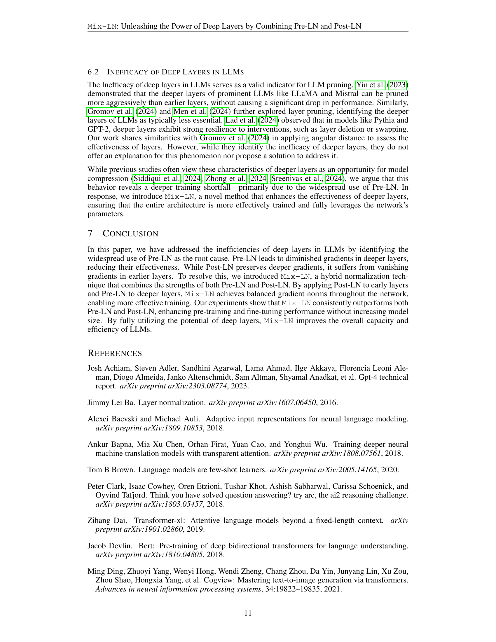
🔼 This figure, located in Section 5 (Analysis and More Evaluations), visualizes the gradient norms of layers within the LLaMA-250M model. It compares the gradient norms of each layer under various layer normalization techniques including Pre-LN, Post-LN and the proposed Mix-LN. The figure is intended to show the impact of different normalization techniques on gradient flow and stability of training.
read the caption
(a) Layer gradient norm of LLaMA-250M with various normalization techniques.

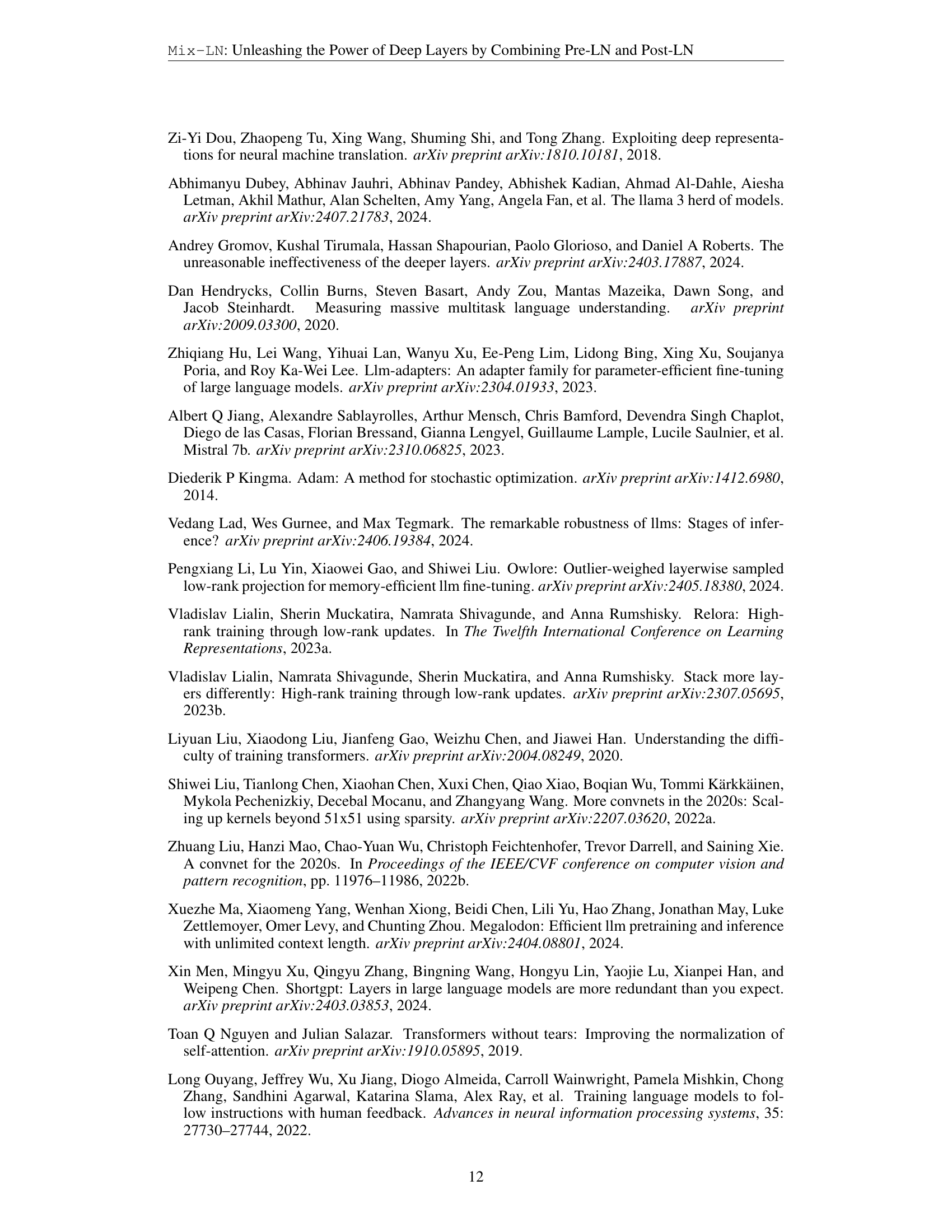
🔼 This figure compares the performance drop (reduction in ARC-e accuracy after supervised fine-tuning) when individual layers are pruned from a 130M parameter LLaMA model. Three normalization methods are compared: Pre-LN, Post-LN, and the proposed Mix-LN. The x-axis represents the index of the layer being pruned, and the y-axis represents the change in ARC-e score. A larger drop indicates the layer is more important for performance. Mix-LN shows greater performance drops for deeper layers than Pre-LN, suggesting that deeper layers are better utilized and contribute more meaningfully when using Mix-LN.
read the caption
(b) Performance drop comparison of LLaMA-130M across layers for Pre-LN, Post-LN, and Mix-LN.
More on tables
| Method | MMLU | BoolQ | ARC-e | PIQA | Hellaswag | OBQA | Winogrande | Avg. |
|---|---|---|---|---|---|---|---|---|
| LLaMA-250M | ||||||||
| Post-LN | 22.95 | 37.83 | 26.94 | 52.72 | 26.17 | 11.60 | 49.56 | 32.54 |
| DeepNorm | 23.60 | 37.86 | 36.62 | 61.10 | 25.69 | 15.00 | 49.57 | 35.63 |
| Pre-LN | 24.93 | 38.35 | 40.15 | 63.55 | 26.34 | 16.20 | 49.01 | 36.93 |
| Mix-LN | 26.53 | 56.12 | 41.68 | 66.34 | 30.16 | 18.00 | 50.56 | 41.34 |
| LLaMA-1B | ||||||||
| Post-LN | 22.95 | 37.82 | 25.08 | 49.51 | 25.04 | 13.80 | 49.57 | 31.96 |
| DeepNorm | 23.35 | 37.83 | 27.06 | 52.94 | 26.19 | 11.80 | 49.49 | 32.67 |
| Pre-LN | 26.54 | 62.20 | 45.70 | 67.79 | 30.96 | 17.40 | 50.51 | 43.01 |
| Mix-LN | 27.99 | 61.93 | 48.11 | 68.50 | 31.35 | 18.80 | 55.93 | 44.66 |
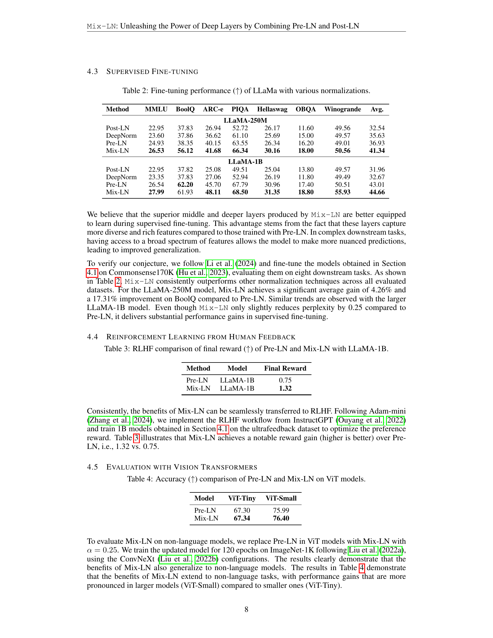
🔼 This table presents the fine-tuning performance of LLaMa models with different normalization methods on eight downstream tasks: MMLU, BoolQ, ARC-e, PIQA, HellaSwag, OBQA, and Winogrande. It includes results for two LLaMa model sizes (250M and 1B parameters) and four normalization strategies (Post-LN, DeepNorm, Pre-LN, and Mix-LN). The average performance across all tasks is also provided. Higher scores indicate better performance.
read the caption
Table 2: Fine-tuning performance (↑↑\uparrow↑) of LLaMa with various normalizations.
| Method | Model | Final Reward |
|---|---|---|
| Pre-LN | LLaMA-1B | 0.75 |
| Mix-LN | LLaMA-1B | 1.32 |
🔼 This table compares the final reward achieved by Large Language Models (LLMs) after Reinforcement Learning from Human Feedback (RLHF) training. Specifically, it presents the results for LLaMA-1B models trained with two different layer normalization methods: Pre-LN (Pre-Layer Normalization) and Mix-LN (the proposed method). The reward is a metric used to assess the quality of the generated text, with higher reward values generally indicating better performance. This comparison aims to demonstrate the effectiveness of Mix-LN in improving the quality of LLMs fine-tuned with RLHF.
read the caption
Table 3: RLHF comparison of final reward (↑↑\uparrow↑) of Pre-LN and Mix-LN with LLaMA-1B.
| Model | ViT-Tiny | ViT-Small |
|---|---|---|
| Pre-LN | 67.30 | 75.99 |
| Mix-LN | 67.34 | 76.40 |
🔼 This table compares the accuracy of Vision Transformer (ViT) models using two different layer normalization methods: Pre-LN (pre-layer normalization) and Mix-LN (mixed layer normalization). Mix-LN is a novel technique introduced in this paper that combines Pre-LN and Post-LN to improve performance. The table presents accuracy scores for two ViT model sizes (ViT-Tiny and ViT-Small) when trained on the ImageNet-1K dataset. The goal is to demonstrate that the benefits of Mix-LN extend beyond language models to other domains like computer vision.
read the caption
Table 4: Accuracy (↑↑\uparrow↑) comparison of Pre-LN and Mix-LN on ViT models.
| Post-LN ratios | Pre-LN | Mix-LN | Mix-LN | Mix-LN | Mix-LN | Mix-LN | Post-LN |
|---|---|---|---|---|---|---|---|
| 0 | 16.7% | 25.0% | 33.0% | 41.7% | 50.0% | 100% | |
| Perplexity | 18.65 | 18.34 | 18.18 | 18.41 | 18.55 | 18.86 | 1434 |
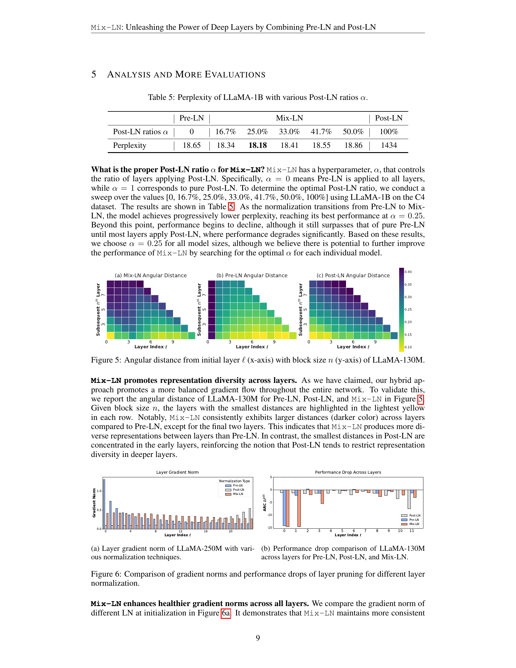
🔼 This table presents the perplexity scores achieved by the LLaMA-1B model when trained with different Post-LN ratios (α). The α parameter controls the proportion of layers in the model that utilize Post-Layer Normalization, while the remaining layers use Pre-Layer Normalization. A ratio of 0 corresponds to using Pre-LN for all layers, whereas a ratio of 1 represents using Post-LN for all layers. Intermediate values create a mix of Pre-LN and Post-LN within the model. The table compares the performance of these mixed normalization strategies against the baseline performance of pure Pre-LN and Post-LN. Lower perplexity scores indicate better performance. The purpose of this analysis is to demonstrate the performance benefits of the proposed Mix-LN approach over standard Pre-LN and Post-LN, as well as to find the optimal balance between the two normalization methods.
read the caption
Table 5: Perplexity of LLaMA-1B with various Post-LN ratios α𝛼\alphaitalic_α.
| Model | Pre-LN | Admin | Group-LN | Sandwich-LN | Mix-LN |
|---|---|---|---|---|---|
| LLaMA-250M | 23.39 | 24.82 | 23.10 | 23.26 | 22.33 |
🔼 This table compares the perplexity scores of the LLaMA-250M model when trained with different normalization methods including Pre-LN, Admin, Group-LN, Sandwich-LN and the proposed Mix-LN. The results highlight the effectiveness of Mix-LN in achieving lower perplexity compared to other recent normalization techniques.
read the caption
Table 6: Comparison against other normalization methods on LLaMA-250M.
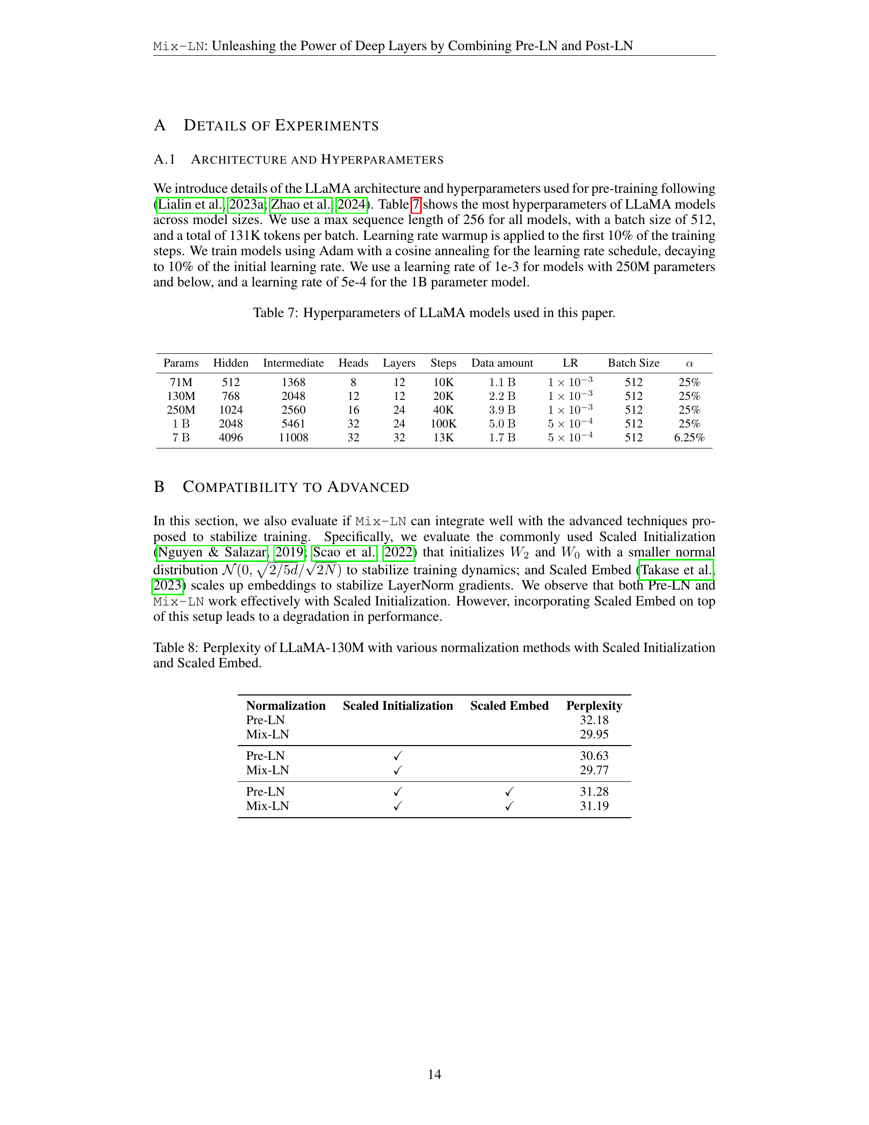
| Params | Hidden | Intermediate | Heads | Layers | Steps | Data amount | LR | Batch Size | []alpha |
|---|---|---|---|---|---|---|---|---|---|
| 71M | 512 | 1368 | 8 | 12 | 10K | 1.1B | 1e-3 | 512 | 25% |
| 130M | 768 | 2048 | 12 | 12 | 20K | 2.2B | 1e-3 | 512 | 25% |
| 250M | 1024 | 2560 | 16 | 24 | 40K | 3.9B | 1e-3 | 512 | 25% |
| 1B | 2048 | 5461 | 32 | 24 | 100K | 5.0B | 5e-4 | 512 | 25% |
| 7B | 4096 | 11008 | 32 | 32 | 13K | 1.7B | 5e-4 | 512 | 6.25% |
🔼 This table, located in Appendix A.1, details the hyperparameters used for pre-training different sizes of LLaMA models, following configurations from Lialin et al. (2023a) and Zhao et al. (2024). It outlines the model size (in parameters), hidden size, intermediate size, number of heads, number of layers, training steps, data amount, learning rate, batch size, and the Post-LN ratio (α) used for Mix-LN experiments. The table shows how these hyperparameters vary across different model sizes, from 71M to 7B parameters, and provides context for understanding the experimental setup and results discussed in the paper. The max sequence length was fixed as 256 with a batch size of 512, totaling 131K tokens per batch. A warmup of the learning rate to 10% of the training steps was used. All models are trained using Adam optimizer with cosine annealing for the learning rate schedule, decaying to 10% of the initial value. Different learning rates are used based on the model sizes: 1e-3 for model sizes under 250M and 5e-4 for the 1B model.
read the caption
Table 7: Hyperparameters of LLaMA models used in this paper.
| Normalization | Scaled Initialization | Scaled Embed | Perplexity |
|---|---|---|---|
| Pre-LN | 32.18 | ||
| Mix-LN | 29.95 | ||
| Pre-LN | ✓ | 30.63 | |
| Mix-LN | ✓ | 29.77 | |
| Pre-LN | ✓ | ✓ | 31.28 |
| Mix-LN | ✓ | ✓ | 31.19 |
🔼 This table compares the perplexity of a 130M parameter LLaMA language model trained with different normalization methods, combined with Scaled Initialization and Scaled Embed techniques. Mix-LN consistently shows the lowest perplexity both with and without these additional techniques, demonstrating its compatibility with training stabilizers and ability to improve the overall quality of the model.
read the caption
Table 8: Perplexity of LLaMA-130M with various normalization methods with Scaled Initialization and Scaled Embed.
Full paper#
