↗ arXiv ↗ Hugging Face ↗ Papers with Code
TL;DR#
Monocular depth estimation has seen advancements with depth foundation models, offering high-quality relative depth. However, they suffer from scale ambiguity, hindering real-world applications like autonomous driving and robotics that need accurate metric depth. Existing methods, including finetuning on metric datasets or incorporating camera intrinsics, haven’t fully solved the problem of inconsistent and inaccurate scale.
This paper introduces “Prompt Depth Anything,” a new paradigm using a low-cost LiDAR as a prompt to guide a depth foundation model. A concise prompt fusion architecture integrates LiDAR at multiple scales within the depth decoder. To address the scarcity of training data with both LiDAR and precise ground truth, the authors propose a scalable data pipeline that simulates LiDAR for synthetic data and generates pseudo ground truth for real data using 3D reconstruction and an edge-aware loss. The method achieves state-of-the-art results and benefits 3D reconstruction and robotic grasping.
Key Takeaways#
Why does it matter?#
This paper introduces a novel paradigm shift in metric depth estimation by prompting depth foundation models, like using a low-cost LiDAR sensor as a guide. This approach simplifies metric depth acquisition and offers a practical solution for applications like robotics and 3D reconstruction. The scalable data pipeline proposed also addresses the challenge of limited training data, enabling more robust training of depth estimation models. It opens new research avenues in prompt engineering for depth foundation models and using readily available, low-cost sensors for high-quality depth perception.
Visual Insights#

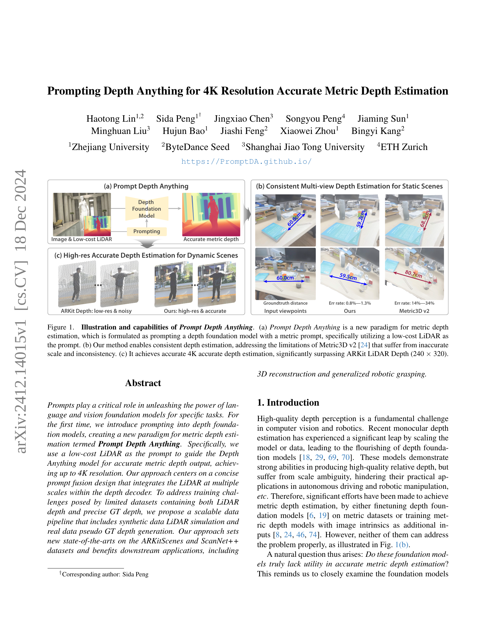
🔼 This figure illustrates the Prompt Depth Anything paradigm and its capabilities. (a) shows the overall framework: a low-cost LiDAR is used as a metric prompt to guide a depth foundation model for accurate metric depth estimation. (b) highlights the consistency of multi-view depth estimation in a static scene, comparing the results of Prompt Depth Anything with Metric3D v2 and ground truth measurements. It demonstrates that Prompt Depth Anything maintains accuracy and consistency across different viewpoints, while Metric3D v2 suffers from scale and consistency issues. (c) demonstrates high-resolution accurate depth estimation in a dynamic scene, comparing Prompt Depth Anything with ARKit LiDAR Depth. Prompt Depth Anything produces high-resolution (4K) and more accurate depth for the moving subject, significantly outperforming the low-resolution (240x320) and noisy output of ARKit LiDAR Depth.
read the caption
Figure 1: Illustration and capabilities of Prompt Depth Anything. (a) Prompt Depth Anything is a new paradigm for metric depth estimation, which is formulated as prompting a depth foundation model with a metric prompt, specifically utilizing a low-cost LiDAR as the prompt. (b) Our method enables consistent depth estimation, addressing the limitations of Metric3D v2 [24] that suffer from inaccurate scale and inconsistency. (c) It achieves accurate 4K accurate depth estimation, significantly surpassing ARKit LiDAR Depth (240 ×\times× 320).
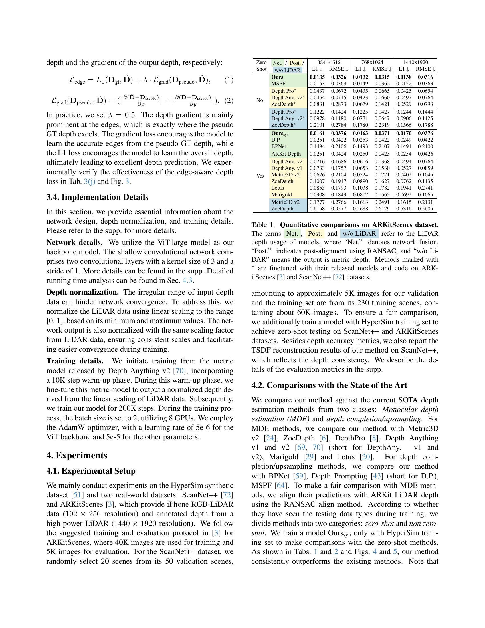
| w/o LiDAR | 384x512 | 768x1024 | 1440x1920 | ||
|---|---|---|---|---|---|
| L1 ↓ | RMSE ↓ | L1 ↓ | RMSE ↓ | L1 ↓ | RMSE ↓ |
| No | Ours | 0.0135 | 0.0326 | 0.0132 | 0.0315 |
| MSPF | 0.0153 | 0.0369 | 0.0149 | 0.0362 | |
| Depth Pro* | 0.0437 | 0.0672 | 0.0435 | 0.0665 | |
| DepthAny. v2* | 0.0464 | 0.0715 | 0.0423 | 0.0660 | |
| ZoeDepth* | 0.0831 | 0.2873 | 0.0679 | 0.1421 | |
| Depth Pro* | 0.1222 | 0.1424 | 0.1225 | 0.1427 | |
| DepthAny. v2* | 0.0978 | 0.1180 | 0.0771 | 0.0647 | |
| ZoeDepth* | 0.2101 | 0.2784 | 0.1780 | 0.2319 | |
| Yes | Ours | 0.0161 | 0.0376 | 0.0163 | 0.0371 |
| D.P. | 0.0251 | 0.0422 | 0.0253 | 0.0422 | |
| BPNet | 0.1494 | 0.2106 | 0.1493 | 0.2107 | |
| ARKit Depth | 0.0251 | 0.0424 | 0.0250 | 0.0423 | |
| DepthAny. v2 | 0.0716 | 0.1686 | 0.0616 | 0.1368 | |
| DepthAny. v1 | 0.0733 | 0.1757 | 0.0653 | 0.1530 | |
| Metric3D v2 | 0.0626 | 0.2104 | 0.0524 | 0.1721 | |
| ZoeDepth | 0.1007 | 0.1917 | 0.0890 | 0.1627 | |
| Lotus | 0.0853 | 0.1793 | 0.1038 | 0.1782 | |
| Marigold | 0.0908 | 0.1849 | 0.0807 | 0.1565 | |
| Metric3D v2 | 0.1777 | 0.2766 | 0.1663 | 0.2491 | |
| ZoeDepth | 0.6158 | 0.9577 | 0.5688 | 0.6129 |
🔼 This table presents a quantitative comparison of various depth estimation methods on the ARKitScenes dataset. The methods are categorized by their usage of LiDAR data: Network fusion integrates LiDAR within the model, Post-alignment uses LiDAR with RANSAC for refinement after initial depth prediction, and w/o LiDAR indicates methods that don’t use LiDAR but produce metric depth directly. Methods marked with an asterisk have been fine-tuned on both ARKitScenes and ScanNet++ datasets. The table columns represent different output resolutions and metrics for depth evaluation. ‘Zero Shot’ denotes models that predict depth in a zero-shot manner and ‘Ours_syn’ represents a model trained only on synthetic data. The metrics include L1 loss, RMSE, relative depth error. The lower the better for those metrics.
read the caption
Table 1: Quantitative comparisons on ARKitScenes dataset. The terms Net., Post. and w/o LiDAR refer to the LiDAR depth usage of models, where “Net.” denotes network fusion, “Post.” indicates post-alignment using RANSAC, and “w/o LiDAR” means the output is metric depth. Methods marked with ∗ are finetuned with their released models and code on ARKitScenes [3] and ScanNet++ [72] datasets.
In-depth insights#
Prompting 4K Depth#
Prompting 4K Depth explores a novel paradigm in depth estimation by leveraging the power of foundation models like Depth Anything. Instead of training from scratch, the model is prompted with low-cost LiDAR data, serving as a metric guide. This approach allows for achieving high-resolution (4K) metric depth estimation, overcoming limitations of traditional monocular methods. Key innovations include a multi-scale prompt fusion architecture within the model’s decoder, effectively integrating LiDAR information. The training process addresses data scarcity by using synthetic LiDAR simulation and pseudo ground truth generation. Results on ARKitScenes and ScanNet++ demonstrate state-of-the-art performance, highlighting the potential of this prompting approach for various applications, including 3D reconstruction and robotic grasping.
LiDAR Fusion Arch.#
LiDAR Fusion Arch. would explore innovative architectures for integrating LiDAR data into depth estimation models. A key challenge is effectively fusing the sparse, noisy LiDAR data with the dense image information. Architectures could range from simple concatenation to more sophisticated attention mechanisms, leveraging transformers or graph neural networks to exploit spatial relationships. Multi-scale fusion, incorporating LiDAR at different resolutions, might further improve accuracy and robustness. Designing lightweight, real-time compatible architectures would be crucial for practical applications like robotics and augmented reality.
Scalable Data Pipeline#
The scalable data pipeline addresses the challenge of training data scarcity for metric depth estimation. Existing datasets lack either LiDAR data or accurate ground truth. This pipeline enhances data diversity and quality through two key processes. First, it simulates low-resolution, noisy LiDAR data for synthetic datasets with precise ground truth, making them suitable for training. Second, it generates pseudo ground truth for real-world LiDAR datasets lacking accurate depth annotations by employing 3D reconstruction. This innovative approach ensures the pipeline’s scalability and robustness, producing high-quality training data for diverse scenarios and ultimately enabling more accurate metric depth estimation.
Edge-Aware Depth#
Edge-aware depth estimation focuses on accurately predicting depth values, especially at object boundaries and edges where depth discontinuities occur. Traditional methods often smooth over these edges, leading to blurry or inaccurate depth maps. However, preserving edge information is crucial for various applications like 3D reconstruction, object recognition, and scene understanding. By incorporating edge information, the depth estimation model can produce sharper, more realistic depth maps. This can be achieved by incorporating edge detection or image gradients into the depth estimation pipeline, or by using specific loss functions that penalize errors at edges more heavily. Edge-aware depth estimation significantly improves the quality and usefulness of depth maps, enabling more accurate and detailed representations of the 3D world.
Zero-Shot Transfer#
Zero-shot transfer in depth estimation aims to apply a model trained on one dataset to a new, unseen dataset without further training. This capability is crucial for generalization and real-world deployment, where retraining on every new environment is impractical. Achieving robust zero-shot performance requires models to learn intrinsic scene properties rather than overfit to specific dataset characteristics. This can be facilitated by diverse training data, suitable model architectures, and training procedures that encourage generalization, like appropriate data augmentation and regularization techniques. While some progress has been made, significant challenges remain, particularly in handling variations in lighting, texture, and object types across different datasets. Robust zero-shot transfer remains a key area for future research, promising more versatile and adaptable depth estimation models.
More visual insights#
More on figures

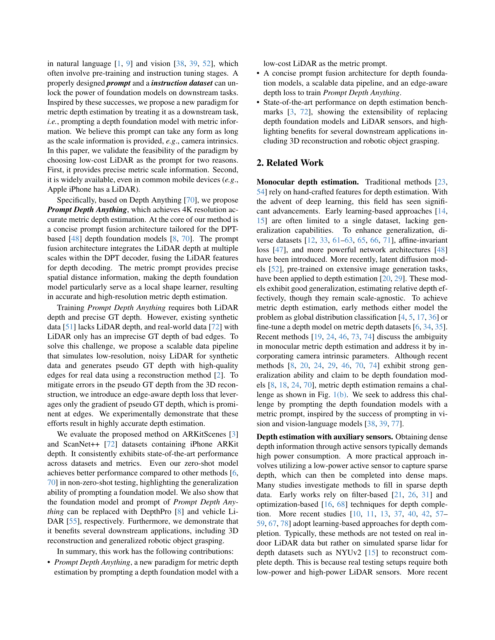
🔼 Prompt Depth Anything uses a low-cost LiDAR as a prompt to guide a depth foundation model for accurate metric depth output, achieving a resolution up to 4K. This is achieved using a multi-scale prompt fusion design within the model’s architecture, specifically a DPT decoder. The training process involves a scalable data pipeline that addresses the challenge of limited datasets containing both LiDAR and precise ground truth depth. This pipeline uses synthetic data LiDAR simulation, real data pseudo ground truth depth generation, and an edge-aware depth loss function that leverages pseudo and annotated ground truth data.
read the caption
Figure 2: Overview of Prompt Depth Anything. (a) Prompt Depth Anything builds on a depth foundation model [70] with a ViT encoder and a DPT decoder, and adds a multi-scale prompt fusion design, using a prompt fusion block to fuse the metric information at each scale. (b) Since training requires both low-cost LiDAR and precise GT depth, we propose a scalable data pipeline that simulates LiDAR depth for synthetic data with precise GT depth, and generates pseudo GT depth for real data with LiDAR. An edge-aware depth loss is proposed to merge accurate edges from pseudo GT depth with accurate depth in textureless areas from FARO annotated GT depth on real data.

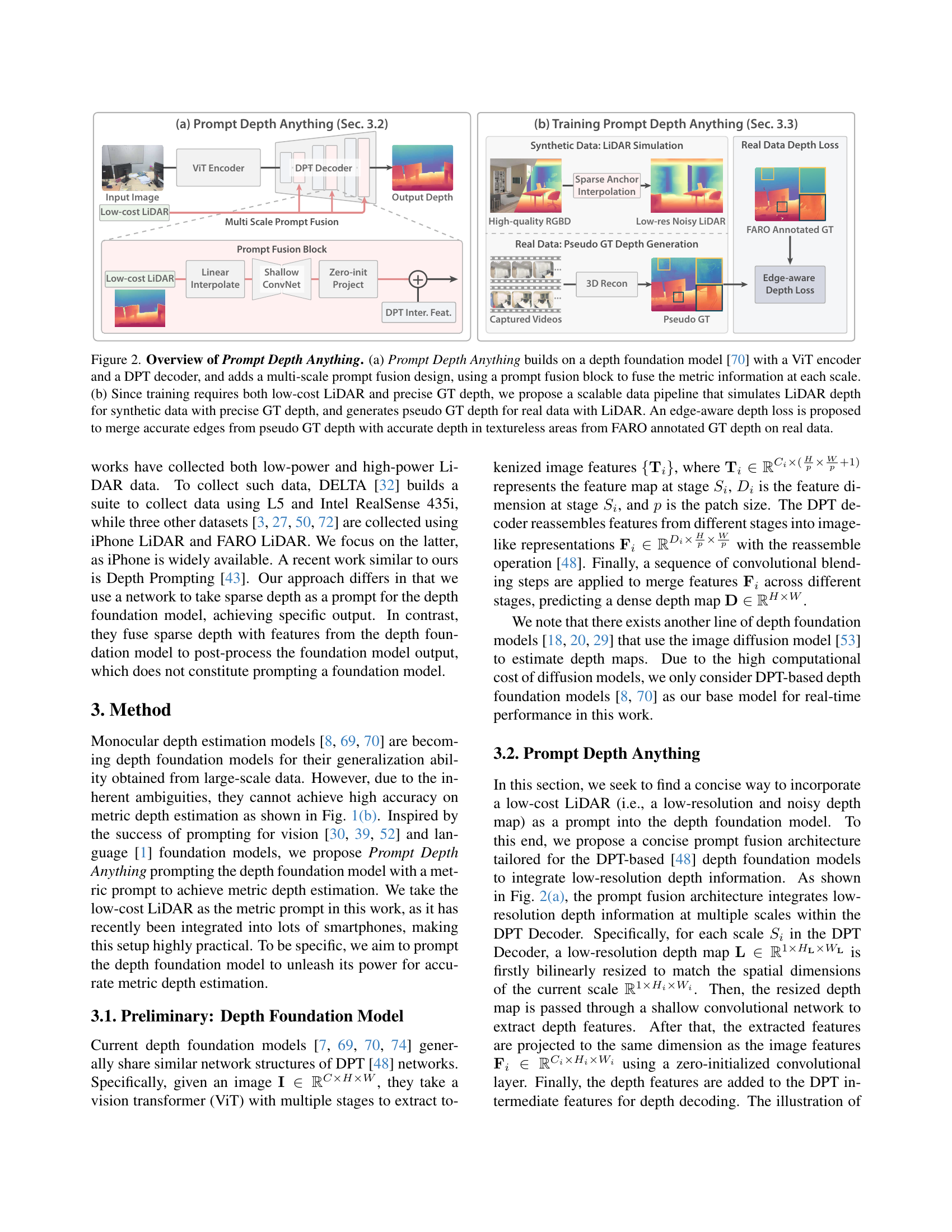
🔼 This figure shows the effect of using sparse anchor interpolation for LiDAR simulation and pseudo ground truth depth generation with edge-aware depth loss. It includes two examples, one for synthetic data and one for real-world data. In each example, the leftmost image is the input RGB image along with the simulated LiDAR depth data represented by colored points. For synthetic data, the middle image shows the depth prediction without sparse anchor interpolation, effectively showcasing depth super-resolution. The right image shows the depth prediction using sparse anchor interpolation, showing accurate depth prediction with simulated LiDAR noise. For real-world data, the middle image shows the depth prediction directly supervised by noisy and hole-filled ground truth depth, resulting in poor depth quality, especially at edges. The right image shows the depth prediction using edge-aware depth loss with pseudo ground truth and noisy ground truth, which yields high-quality edge depth and accurate depth prediction. The two rows emphasize the improvements of using sparse anchor interpolation and edge-aware loss respectively by highlighting their depth prediction improvements at the edges.
read the caption
Figure 3: Effects on the synthetic data lidar simulation and real data pseudo GT generation with the edge-aware depth loss. The middle and right columns are the depth prediction results of our different models. The two rows highlight the significance of sparse anchor interpolation for lidar simulation and pseudo GT generation with edge-aware depth loss, respectively.

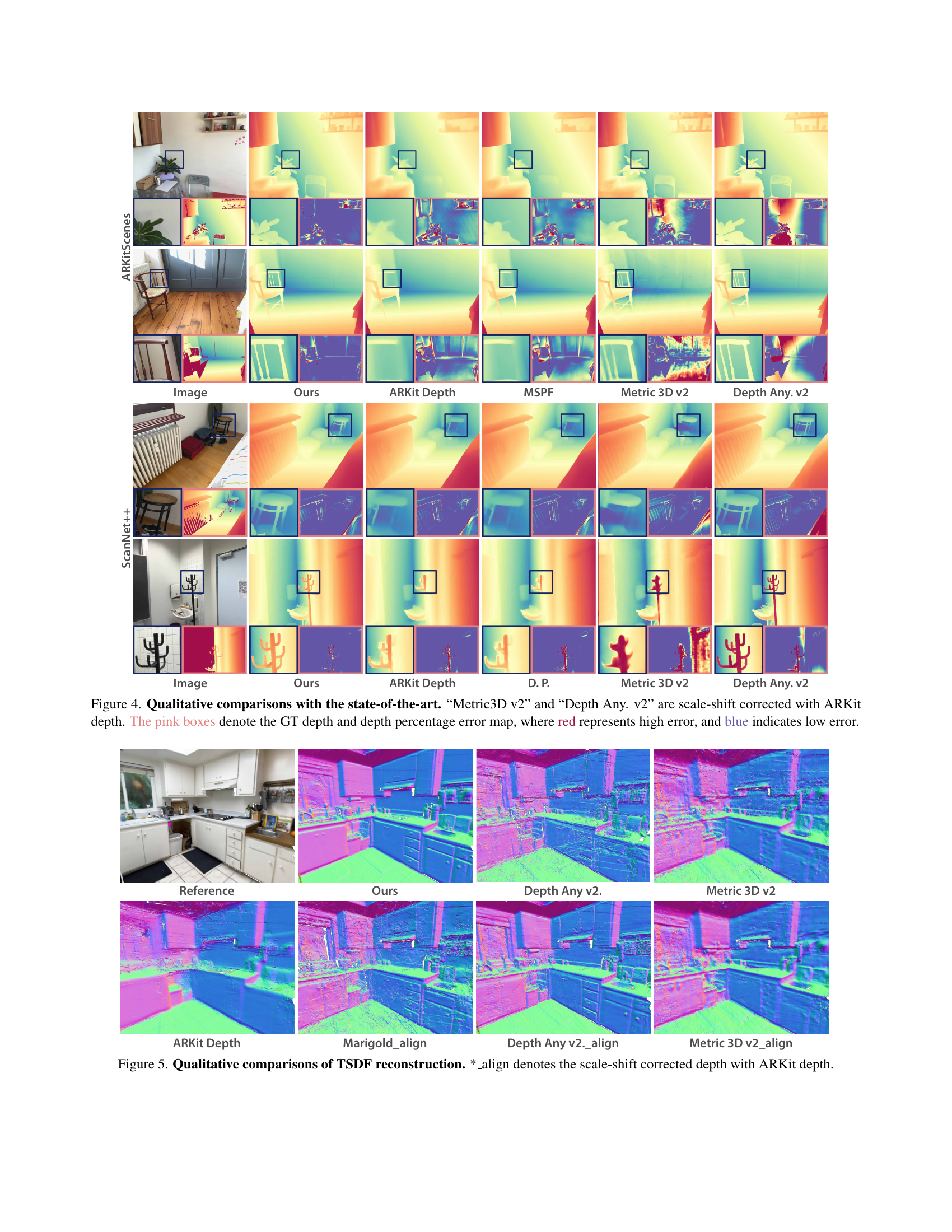
🔼 This figure presents qualitative results of the proposed method comparing with other state-of-the-art methods on two datasets: ARKitScenes and ScanNet++. It contains predicted depth maps from various methods and also ground truth and error maps. We can observe that the proposed method outperforms previous methods significantly, producing more accurate depth maps that faithfully align with the ground truth, and resulting in lower error rates, particularly in challenging areas like thin structures.
read the caption
Figure 4: Qualitative comparisons with the state-of-the-art. “Metric3D v2” and “Depth Any. v2” are scale-shift corrected with ARKit depth. The pink boxes denote the GT depth and depth percentage error map, where red represents high error, and blue indicates low error.

🔼 This figure shows qualitative results of 3D scene reconstruction using the TSDF fusion method with different depth estimation methods. The figure compares the proposed method’s reconstruction quality against Depth Anything v2 and Metric3D v2, highlighting improvements in reconstructing details and overall scene completeness. ‘*_align’ in the caption indicates that the depth maps from monocular depth estimation methods (Marigold, Depth Any v2, Metric 3D v2) are aligned to the scale of ARKit depth using RANSAC to allow for a fair comparison of the metric depth results.
read the caption
Figure 5: Qualitative comparisons of TSDF reconstruction. *_align denotes the scale-shift corrected depth with ARKit depth.

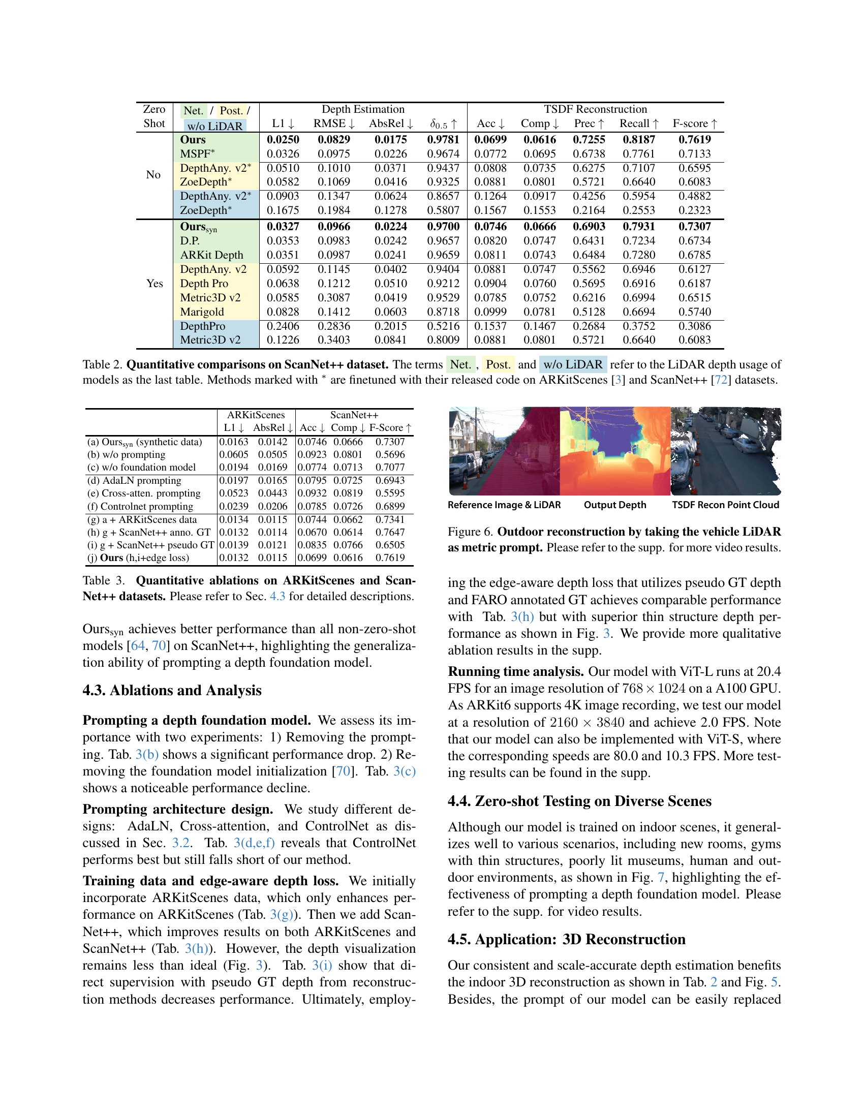
🔼 This figure showcases the 3D reconstruction of an outdoor street scene using vehicle LiDAR as a metric prompt. It demonstrates the application of Prompt Depth Anything to large-scale outdoor environments by replacing the low-cost LiDAR prompt with vehicle LiDAR data and training on the Shift autonomous driving dataset. The top left section shows the input RGB image of the street scene, while the remaining sections display different views of the reconstructed 3D point cloud, illustrating depth and structural details.
read the caption
Figure 6: Outdoor reconstruction by taking the vehicle LiDAR as metric prompt. Please refer to the supp. for more video results.

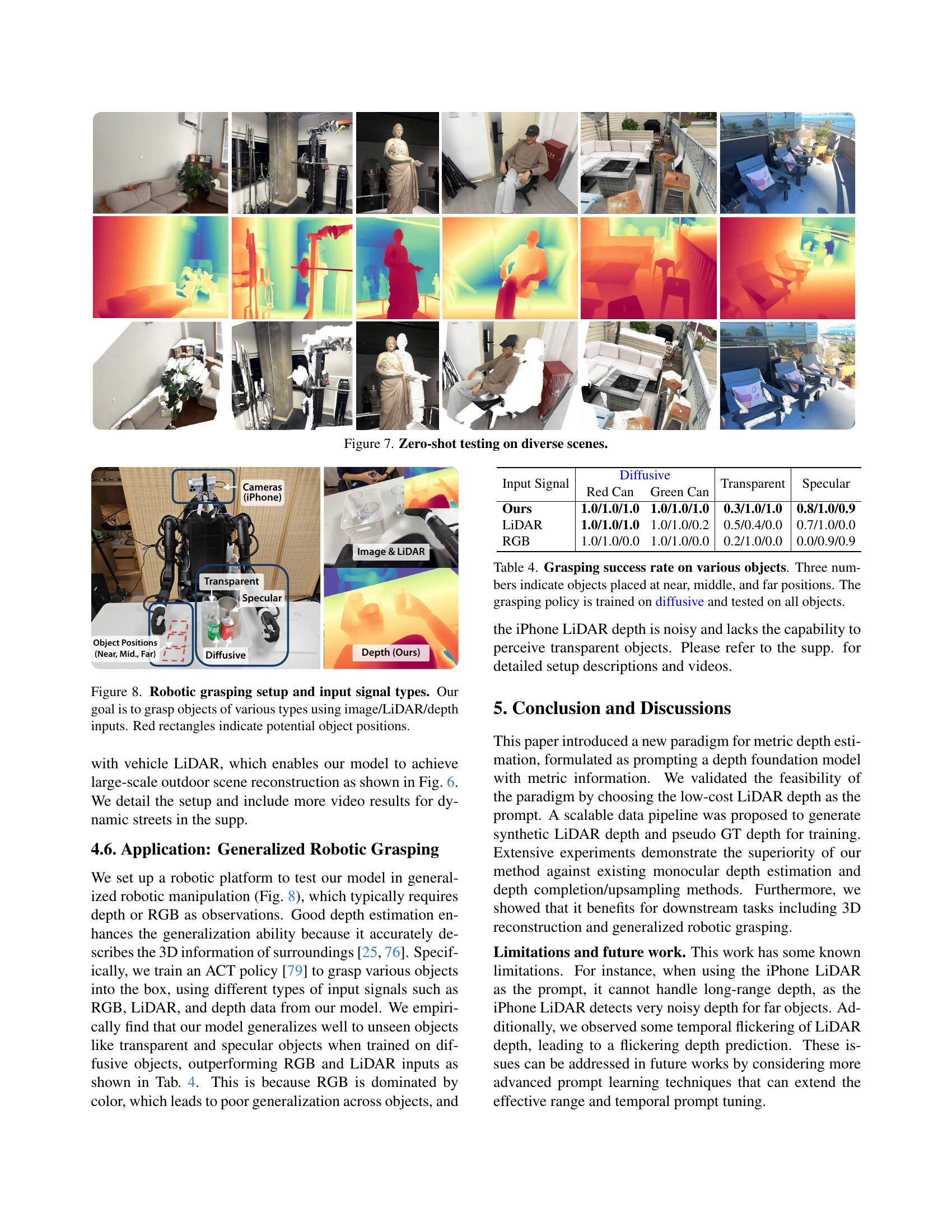
🔼 This figure showcases the zero-shot performance of Prompt Depth Anything on a diverse range of scenes, highlighting the model’s robustness and generalization ability. The scenes depicted include indoor environments with challenging lighting and thin structures (rooms, gyms, and museums), and extend to outdoor environments and human subjects.
read the caption
Figure 7: Zero-shot testing on diverse scenes.

🔼 This figure illustrates the robotic grasping setup used in the experiments. The setup involves a robotic arm tasked with grasping objects of varying properties (transparent, specular, diffusive) placed at different distances (near, mid, far). The input signals used for controlling the robotic arm are: RGB images from a camera, LiDAR depth data, and the monocular depth estimations generated by the proposed model. The red rectangles highlight potential positions of the objects.
read the caption
Figure 8: Robotic grasping setup and input signal types. Our goal is to grasp objects of various types using image/LiDAR/depth inputs. Red rectangles indicate potential object positions.

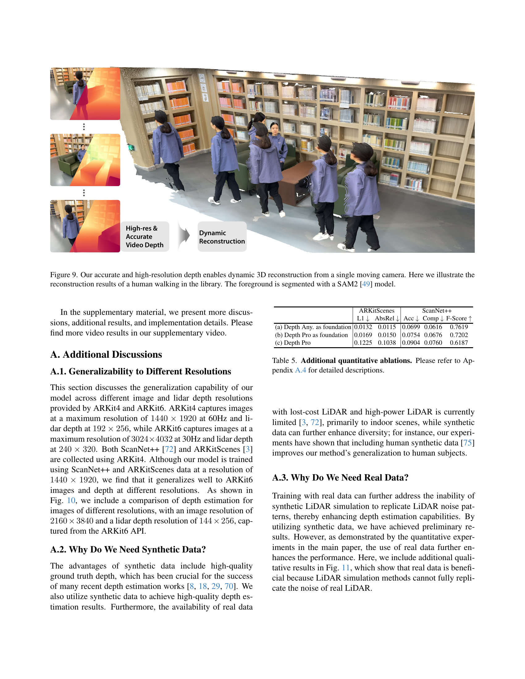
🔼 This figure demonstrates the capability of the proposed method to perform dynamic 3D reconstruction of a human subject walking in a library setting using a single moving camera. The high accuracy and resolution of the depth map facilitate precise 3D reconstruction, and SAM2 is employed to segment the foreground, effectively separating the human subject from the background.
read the caption
Figure 9: Our accurate and high-resolution depth enables dynamic 3D reconstruction from a single moving camera. Here we illustrate the reconstruction results of a human walking in the library. The foreground is segmented with a SAM2 [49] model.

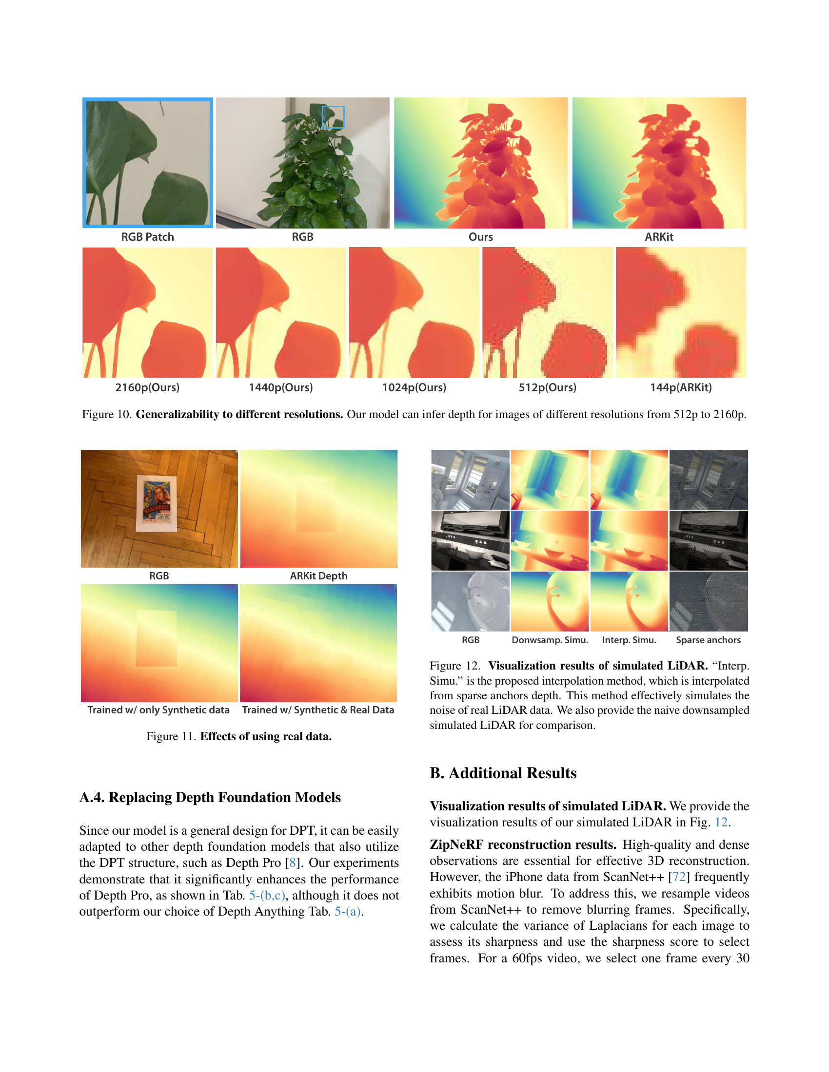
🔼 This figure shows the results of applying Prompt Depth Anything to images of different resolutions from 512p to 2160p, including RGB image, the predicted depth by the model, and the LiDAR depth provided by the iPhone. Even with higher resolution input, Prompt Depth Anything predicts plausible depth estimations, showing its generalizability to different resolutions.
read the caption
Figure 10: Generalizability to different resolutions. Our model can infer depth for images of different resolutions from 512p to 2160p.

🔼 This figure illustrates the improvement of adding real data to train the model by showing two qualitative results on plants. The top row shows the input RGB image and the predicted depth using ARKit. The bottom row shows the model output trained with only synthetic data and trained with both synthetic and real data, respectively. It demonstrates that real data improves the quality of the edges of the plant, while training with synthetic data only has good performance on flat regions.
read the caption
Figure 11: Effects of using real data.

🔼 This figure visualizes different methods for simulating LiDAR data, comparing a naive downsampling approach with the proposed sparse anchor interpolation method. The naive approach involves directly downsampling the high-resolution depth map to a lower resolution, which fails to capture the noise characteristics of real LiDAR data. In contrast, the sparse anchor interpolation method first downsamples the depth map and then samples points on this map using a distorted grid. The remaining depth values are interpolated from these sampled points using RGB similarity with KNN. This approach effectively simulates the noise present in real LiDAR data, resulting in more realistic simulated LiDAR depth maps for training depth estimation models. The figure includes visualizations of RGB image patch, full RGB image, depth output from the proposed model, and depth from ARKit.
read the caption
Figure 12: Visualization results of simulated LiDAR. “Interp. Simu.” is the proposed interpolation method, which is interpolated from sparse anchors depth. This method effectively simulates the noise of real LiDAR data. We also provide the naive downsampled simulated LiDAR for comparison.

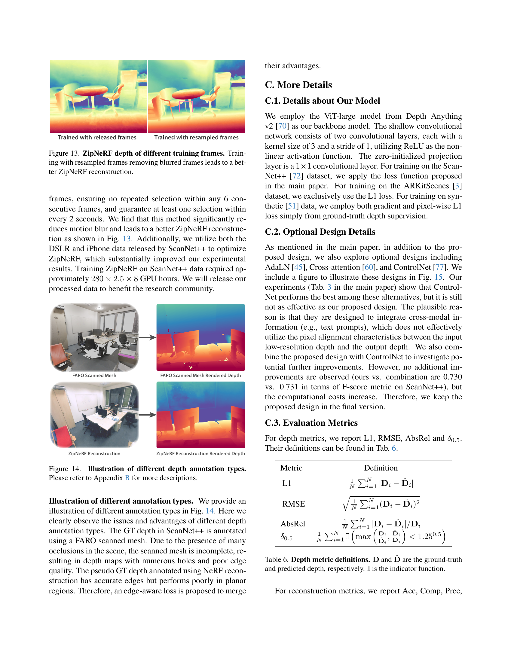
🔼 This figure shows the effect of training ZipNeRF with different frames. The left image shows the result when trained with original frames which include blurred frames. The right image shows the result when trained with resampled frames which remove the blurred ones. Training with resampled frames yield better reconstruction quality.
read the caption
Figure 13: ZipNeRF depth of different training frames. Training with resampled frames removing blurred frames leads to a better ZipNeRF reconstruction.

🔼 This figure shows three different types of depth annotations used for training: (1) Ground Truth (GT) from FARO scanned mesh, which suffers from incompleteness and poor edge quality due to occlusions during scanning. (2) Pseudo GT generated using NeRF reconstruction, which shows better edges compared to GT, but struggles with planar regions. (3) ZipNeRF reconstruction which was trained with resampled frames. It has been observed that resampling frames removes blurring and improves reconstruction.
read the caption
Figure 14: Illustration of different depth annotation types. Please refer to Appendix B for more descriptions.

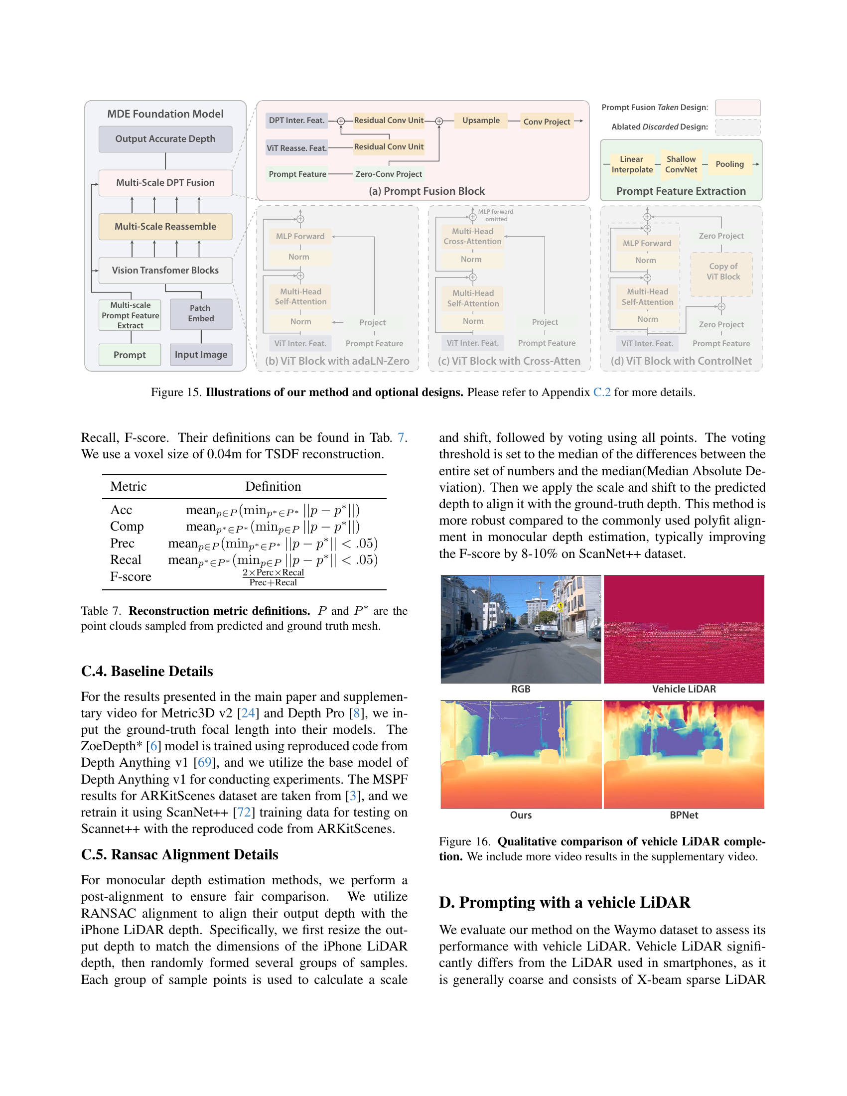
🔼 This figure illustrates the architecture of Prompt Depth Anything and optional designs for incorporating a low-resolution depth map as a prompt into a depth foundation model. (a) The Prompt Fusion Block integrates the low-resolution depth information at multiple scales within the DPT Decoder. The block design takes a low-resolution depth map, resizes it, passes it through a shallow convolutional network, projects it to the same dimension as the image features, and adds the resulting depth features to the DPT intermediate features. Optional designs for prompting architecture are: (b) Adapting the Layer Normalization parameters of the encoder based on the conditioning input. (c) Injecting a cross-attention block after each self-attention block and integrating the conditioning input via cross-attention. (d) Copying the encoder blocks and inputting control signals to the copied blocks to control the output depth.
read the caption
Figure 15: Illustrations of our method and optional designs. Please refer to Sec. C.2 for more details.
More on tables
| Zero Shot | Net. / Post. / w/o LiDAR | Depth Estimation | TSDF Reconstruction | |||||
|---|---|---|---|---|---|---|---|---|
| L1 ↓ | RMSE ↓ | AbsRel ↓ | [ | |||||
| delta_{0.5} ] ↑ | Acc ↓ | Comp ↓ | Prec ↑ | Recall ↑ | F-score ↑ | |||
| No | Ours | 0.0250 | 0.0829 | 0.0175 | 0.9781 | 0.0699 | 0.0616 | 0.7255 |
| MSPF* | 0.0326 | 0.0975 | 0.0226 | 0.9674 | 0.0772 | 0.0695 | 0.6738 | |
| DepthAny. v2* | 0.0510 | 0.1010 | 0.0371 | 0.9437 | 0.0808 | 0.0735 | 0.6275 | |
| ZoeDepth* | 0.0582 | 0.1069 | 0.0416 | 0.9325 | 0.0881 | 0.0801 | 0.5721 | |
| DepthAny. v2* | 0.0903 | 0.1347 | 0.0624 | 0.8657 | 0.1264 | 0.0917 | 0.4256 | |
| ZoeDepth* | 0.1675 | 0.1984 | 0.1278 | 0.5807 | 0.1567 | 0.1553 | 0.2164 | |
| Yes | Ourssyn | 0.0327 | 0.0966 | 0.0224 | 0.9700 | 0.0746 | 0.0666 | 0.6903 |
| D.P. | 0.0353 | 0.0983 | 0.0242 | 0.9657 | 0.0820 | 0.0747 | 0.6431 | |
| ARKit Depth | 0.0351 | 0.0987 | 0.0241 | 0.9659 | 0.0811 | 0.0743 | 0.6484 | |
| DepthAny. v2 | 0.0592 | 0.1145 | 0.0402 | 0.9404 | 0.0881 | 0.0747 | 0.5562 | |
| Depth Pro | 0.0638 | 0.1212 | 0.0510 | 0.9212 | 0.0904 | 0.0760 | 0.5695 | |
| Metric3D v2 | 0.0585 | 0.3087 | 0.0419 | 0.9529 | 0.0785 | 0.0752 | 0.6216 | |
| Marigold | 0.0828 | 0.1412 | 0.0603 | 0.8718 | 0.0999 | 0.0781 | 0.5128 | |
| DepthPro | 0.2406 | 0.2836 | 0.2015 | 0.5216 | 0.1537 | 0.1467 | 0.2684 | |
| Metric3D v2 | 0.1226 | 0.3403 | 0.0841 | 0.8009 | 0.0881 | 0.0801 | 0.5721 |
🔼 This table presents a quantitative evaluation of various depth estimation models on the ScanNet++ dataset. The metrics used for evaluation include L1, RMSE, AbsRel, Accuracy (Acc.), Completeness (Comp.), Precision (Prec.), Recall, and F-score. The table categorizes the models based on their usage of LiDAR data (Net.: Network Fusion; Post.: Post-alignment; w/o LiDAR: metric depth output without LiDAR input). Some models were finetuned using additional datasets (ARKitScenes and ScanNet++). The zero-shot models, denoted as ‘Ourssyn’ and others, were trained on synthetic data only. The table aims to showcase the effectiveness of the proposed method, ‘Ours,’ in comparison to existing state-of-the-art methods for depth estimation.
read the caption
Table 2: Quantitative comparisons on ScanNet++ dataset. The terms Net., Post. and w/o LiDAR refer to the LiDAR depth usage of models as the last table. Methods marked with ∗ are finetuned with their released code on ARKitScenes [3] and ScanNet++ [72] datasets.
| ARKitScenes | ScanNet++ | ||||
|---|---|---|---|---|---|
| L1 ↓ | AbsRel ↓ | Acc ↓ | Comp ↓ | F-Score ↑ | |
| —: | —: | —: | —: | —: | —: |
| (a) Ourssyn (synthetic data) | 0.0163 | 0.0142 | 0.0746 | 0.0666 | 0.7307 |
| (b) w/o prompting | 0.0605 | 0.0505 | 0.0923 | 0.0801 | 0.5696 |
| (c) w/o foundation model | 0.0194 | 0.0169 | 0.0774 | 0.0713 | 0.7077 |
| (d) AdaLN prompting | 0.0197 | 0.0165 | 0.0795 | 0.0725 | 0.6943 |
| (e) Cross-atten. prompting | 0.0523 | 0.0443 | 0.0932 | 0.0819 | 0.5595 |
| (f) Controlnet prompting | 0.0239 | 0.0206 | 0.0785 | 0.0726 | 0.6899 |
| (g) a + ARKitScenes data | 0.0134 | 0.0115 | 0.0744 | 0.0662 | 0.7341 |
| (h) g + ScanNet++ anno. GT | 0.0132 | 0.0114 | 0.0670 | 0.0614 | 0.7647 |
| (i) g + ScanNet++ pseudo GT | 0.0139 | 0.0121 | 0.0835 | 0.0766 | 0.6505 |
| (j) Ours (h,i+edge loss) | 0.0132 | 0.0115 | 0.0699 | 0.0616 | 0.7619 |
🔼 This table presents the ablation study results of the proposed method, Prompt Depth Anything, quantitatively evaluated on ARKitScenes and ScanNet++ datasets using L1, AbsRel, Acc, Comp, and F-score metrics. Different settings are explored including: using synthetic data only, removing prompting, removing foundation model pre-training, using different prompting architectures (AdaLN, Cross-Attention, and ControlNet), and using and combining different real datasets (ARKitScenes and ScanNet++ with annotated and pseudo ground truth). The table analyzes the impact of prompting a depth foundation model, different architecture designs, training data, and an edge-aware loss on the performance.
read the caption
Table 3: Quantitative ablations on ARKitScenes and ScanNet++ datasets. Please refer to Sec. 4.3 for detailed descriptions.
| Input Signal | Diffusive | Diffusive | Transparent | Specular |
|---|---|---|---|---|
| Red Can | Green Can | |||
| Ours | 1.0/1.0/1.0 | 1.0/1.0/1.0 | 0.3/1.0/1.0 | 0.8/1.0/0.9 |
| LiDAR | 1.0/1.0/1.0 | 1.0/1.0/0.2 | 0.5/0.4/0.0 | 0.7/1.0/0.0 |
| RGB | 1.0/1.0/0.0 | 1.0/1.0/0.0 | 0.2/1.0/0.0 | 0.0/0.9/0.9 |
🔼 This table presents the grasping success rates of a robotic arm attempting to grasp various objects (Red Can, Green Can, Transparent, Specular) placed at different distances (Near, Mid, and Far). The grasping policy used was trained only on diffusive objects (red and green cans). The success rate is evaluated by how often the robot places each object into the designated box from the positions near, middle, and far. The table shows that depth data obtained from the proposed model generally exhibits better performance compared to using RGB images or LiDAR depth from the iPhone, especially for grasping transparent or specular objects.
read the caption
Table 4: Grasping success rate on various objects. Three numbers indicate objects placed at near, middle, and far positions. The grasping policy is trained on diffusive and tested on all objects.
| ARKitScenes | ARKitScenes | ScanNet++ | ScanNet++ | ScanNet++ | |
|---|---|---|---|---|---|
| L1 ↓ | AbsRel ↓ | Acc ↓ | Comp ↓ | F-Score ↑ | |
| ——————— | ———– | ———– | ——– | ——– | ——– |
| (a) Depth Any. as foundation | 0.0132 | 0.0115 | 0.0699 | 0.0616 | 0.7619 |
| (b) Depth Pro as foundation | 0.0169 | 0.0150 | 0.0754 | 0.0676 | 0.7202 |
| (c) Depth Pro | 0.1225 | 0.1038 | 0.0904 | 0.0760 | 0.6187 |
🔼 This table presents additional quantitative ablation study results on ARKitScenes and ScanNet++ datasets by replacing the depth foundation model from Depth Anything to Depth Pro. It shows that using Depth Anything as the base model yields better performance, as indicated in row (a). It also shows that while DepthPro (with prompting) in row (b) performs better than the original Depth Pro in row (c), it still doesn’t match the performance of Depth Anything with prompting in row (a).
read the caption
Table 5: Additional quantitative ablations. Please refer to Sec. A.4 for detailed descriptions.
| Metric | Definition |
|---|---|
| L1 | $\frac{1}{N}\sum_{i=1}^{N} |
| RMSE | $\sqrt{\frac{1}{N}\sum_{i=1}^{N}(\mathbf{D}{i}-\hat{\mathbf{D}}{i})^{2}}$ |
| AbsRel | $\frac{1}{N}\sum_{i=1}^{N} |
| $\delta_{0.5}$ | $\frac{1}{N}\sum_{i=1}^{N}\mathbb{I}\left(\max\left(\frac{\mathbf{D}{i}}{\hat{\mathbf{D}}{i}},\frac{\hat{\mathbf{D}}{i}}{\mathbf{D}{i}}\right)<1.25^{0.5}\right)$ |
🔼 This table defines the metrics used to evaluate depth estimation performance in the paper. Lower values for L1, RMSE, and AbsRel indicate better performance, while a higher value for δ<0.5 indicates better performance. Specifically: * L1: Average absolute difference between the predicted depth and the ground truth depth. * RMSE: Root mean squared error between the predicted depth and the ground truth depth. * AbsRel: Average relative absolute difference between the predicted depth and the ground truth depth. * δ<0.5: Percentage of pixels where the ratio between the predicted depth and the ground truth depth is within a threshold of 0.5, indicating higher accuracy.
read the caption
Table 6: Depth metric definitions. 𝐃𝐃\mathbf{D}bold_D and 𝐃^^𝐃\hat{\mathbf{D}}over^ start_ARG bold_D end_ARG are the ground-truth and predicted depth, respectively. 𝕀𝕀\mathbb{I}blackboard_I is the indicator function.
| Metric | Definition |
|---|---|
| Acc | $\mbox{mean}{p\in P}(\min{p^{}\in P^{}} |
| Comp | $\mbox{mean}{p^{}\in P^{}}(\min{p\in P} |
| Prec | $\mbox{mean}{p\in P}(\min{p^{}\in P^{}} |
| Recal | $\mbox{mean}{p^{}\in P^{}}(\min{p\in P} |
| F-score | $\frac{2\times\text{Perc}\times\text{Recal}}{\text{Prec}+\text{Recal}}$ |
🔼 This table defines metrics used to evaluate the quality of 3D reconstruction. The metrics compare point clouds P (predicted) and P** (ground truth) and include Accuracy (Acc), Completeness (Comp), Precision (Prec), Recall, and F-score. These metrics measure how well the predicted point cloud aligns with the ground truth point cloud. Lower values for Acc and Comp indicate better performance, while higher values for Prec, Recall and F-score indicate better performance.
read the caption
Table 7: Reconstruction metric definitions. P𝑃Pitalic_P and P∗superscript𝑃P^{*}italic_P start_POSTSUPERSCRIPT ∗ end_POSTSUPERSCRIPT are the point clouds sampled from predicted and ground truth mesh.
Full paper#
