↗ arXiv ↗ Hugging Face ↗ Papers with Code
TL;DR#
Scaling up deep learning models is challenging due to computational limitations. Mixture-of-Experts (MoE) models address this by activating only a subset of parameters, significantly reducing computational costs. However, traditional MoE architectures often rely on non-differentiable routing mechanisms (like TopK), hindering performance and scalability. This has led researchers to explore fully-differentiable alternatives.
This paper introduces ReMoE, a novel MoE architecture that uses a fully differentiable ReLU function for routing. This simple yet effective change enables efficient dynamic allocation of computation and superior scalability. Experiments demonstrate ReMoE consistently outperforms traditional TopK-routed MoE models across various settings, showcasing significant improvements in both performance and scalability. The proposed adaptive L1 regularization effectively controls the sparsity of the model, further enhancing its efficiency.
Key Takeaways#
Why does it matter?#
This paper is important because it presents ReMoE, a novel and effective approach to scaling up Mixture-of-Experts (MoE) models. The fully differentiable nature of ReMoE addresses limitations of existing methods, paving the way for more efficient and scalable AI models. This work is highly relevant to current research trends in large language models and opens new avenues for investigation into more efficient routing mechanisms and improved scalability in deep learning.
Visual Insights#

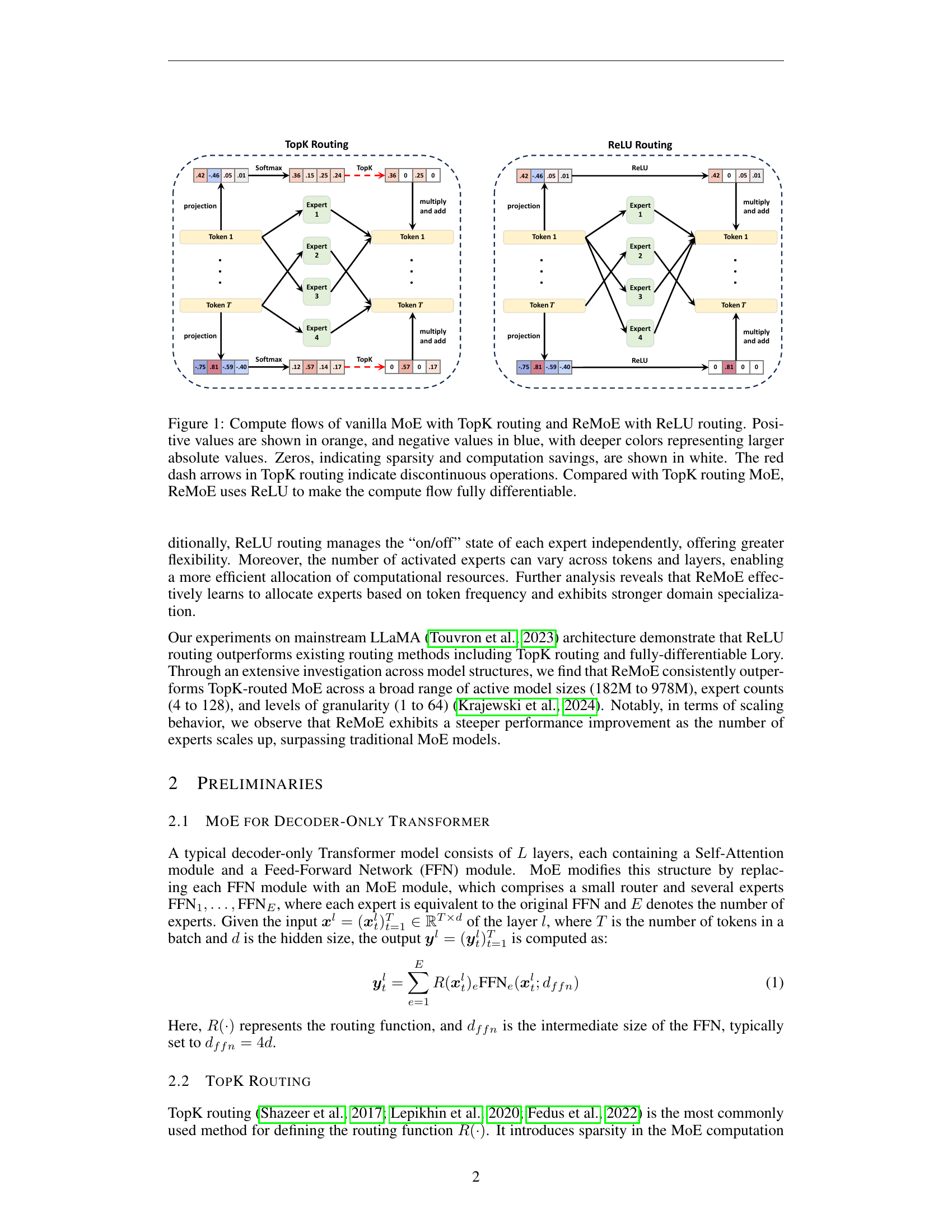
🔼 This figure illustrates the computational flow of both traditional Mixture-of-Experts (MoE) models with TopK routing and the proposed ReMoE model with ReLU routing. The color intensity represents the magnitude of the values, with orange for positive values and blue for negative values. White indicates a zero value, highlighting the sparsity achieved through the selective activation of experts in both architectures. The discontinuous nature of the TopK routing, indicated by dashed red arrows, is a key difference compared to the smooth, continuous computation flow enabled by the ReLU routing in ReMoE, making the training process more efficient.
read the caption
Figure 1: Compute flows of vanilla MoE with TopK routing and ReMoE with ReLU routing. Positive values are shown in orange, and negative values in blue, with deeper colors representing larger absolute values. Zeros, indicating sparsity and computation savings, are shown in white. The red dash arrows in TopK routing indicate discontinuous operations. Compared with TopK routing MoE, ReMoE uses ReLU to make the compute flow fully differentiable.
| Size | #Parameters | hidden_size | num_layers | num_heads | num_groups | GFLOPs |
|---|---|---|---|---|---|---|
| Small | 182M | 768 | 12 | 12 | 4 | 995 |
| Medium | 469M | 1024 | 24 | 16 | 4 | 2873 |
| Large | 978M | 1536 | 24 | 16 | 4 | 5991 |
🔼 This table details the configurations used for the three different sizes of dense backbones in the experiments. The configurations include the number of parameters, the hidden size of the model, the number of layers, the number of heads in the multi-head attention mechanism, the number of groups in the feed-forward network (FFN), and the number of floating point operations (FLOPs) required for a single sequence. FLOPs are calculated using the method described in Narayanan et al. (2021).
read the caption
Table 1: Configurations for the dense backbones. FLOPs are calculated with a single sequence according to Narayanan et al. (2021).
In-depth insights#
MoE’s Differentiability#
The core challenge addressed in the paper is the lack of differentiability in traditional Mixture-of-Experts (MoE) models, specifically those employing TopK routing. This non-differentiable nature stems from the discrete selection process of experts, hindering efficient gradient-based training and limiting the model’s scalability. The authors highlight how the discontinuous softmax and TopK operations create instability during training. To overcome this, they propose ReMoE, which uses a fully differentiable ReLU-based routing mechanism. This crucial change enables smoother transitions between active and inactive expert states, leading to more stable and efficient training. The continuous nature of ReLU routing allows for finer-grained control over expert activation and facilitates a more effective learning process. This differentiability is central to ReMoE’s superior performance and scalability compared to existing methods. The authors emphasize the importance of achieving continuous and smooth transitions for optimal gradient flow, leading to substantial improvements in both training efficiency and model accuracy.
ReLU Routing#
The proposed ReLU routing mechanism offers a fully differentiable alternative to the traditional TopK routing in Mixture-of-Experts (MoE) models. Unlike TopK’s discontinuous softmax and top-k selection, ReLU’s continuous nature allows for smoother gradient flow during training, leading to improved performance and scalability. The use of ReLU gates directly controls expert activation, creating a flexible and dynamic allocation of computational resources across tokens and layers. This adaptability contrasts with TopK’s fixed number of active experts per token. While ReLU’s inherent sparsity needs careful management to control computational cost, the authors address this challenge with an adaptive L1 regularization method. This approach effectively balances sparsity with load balancing, achieving the desired computational efficiency without sacrificing performance. The fully differentiable nature of ReLU routing is a key advantage, enabling more effective model training and potentially unlocking better performance in large-scale MoE architectures.
Sparsity Control#
Effective sparsity control is crucial for Mixture-of-Experts (MoE) models to balance computational efficiency and model capacity. The paper explores this challenge by introducing a novel approach using ReLU routing and a refined L1 regularization. ReLU’s continuous nature enables smoother sparsity adjustments compared to the discontinuous TopK approach, thus improving training stability. The adaptive L1 regularization dynamically adjusts the regularization strength, ensuring that the target sparsity is consistently achieved throughout the training process. This adaptive mechanism is particularly important in mitigating potential issues like routing collapse. By skillfully managing the sparsity, ReMoE effectively balances computational resource allocation across tokens, layers, and experts, leading to improved performance and scalability. The introduction of a load-balancing element into the sparsity control mechanism further enhances its robustness, addressing potential uneven resource distribution among experts. This refined approach is essential for achieving superior scalability and avoiding limitations often encountered in traditional MoE architectures.
Scalability#
The research paper’s findings on scalability reveal that ReMoE consistently outperforms traditional MoE methods across various metrics. Its superior scalability is particularly evident when increasing the number of active parameters, expert count, or granularity. The authors demonstrate that ReMoE’s performance advantage grows more pronounced as these factors scale, suggesting that its fully differentiable nature and dynamic expert allocation strategy are particularly beneficial at larger scales. This improved scalability is attributed to ReMoE’s continuous and fully differentiable ReLU routing, enabling efficient and dynamic resource allocation across tokens and layers. Unlike discontinuous TopK routing, ReMoE’s approach avoids instability and allows for smooth transitions between active and inactive experts, leading to better model training and performance. The adaptive L1 regularization further enhances ReMoE’s scalability by controlling sparsity and promoting load balancing. The study’s results suggest that ReMoE offers a promising approach for scaling up large language models while maintaining efficiency and performance.
Future Work#
Future research directions stemming from the ReMoE paper could explore several avenues. Improving the adaptive L1 regularization is crucial; a more sophisticated method for tuning the sparsity coefficient λ could lead to better control over sparsity and computational cost. Investigating alternative activation functions beyond ReLU for the routing mechanism might offer performance improvements or enhanced stability. The current load-balancing approach is a heuristic; exploring theoretically grounded methods, perhaps leveraging optimal transport theory, could yield more robust and efficient load balancing. Extending ReMoE to other model architectures beyond decoder-only Transformers would demonstrate its broader applicability. Finally, a deeper investigation into the observed three-stage training dynamics and whether this is a general phenomenon applicable to other sparsely activated models deserves attention. Understanding this could lead to optimized training strategies for ReMoE and other MoE models.
More visual insights#
More on figures

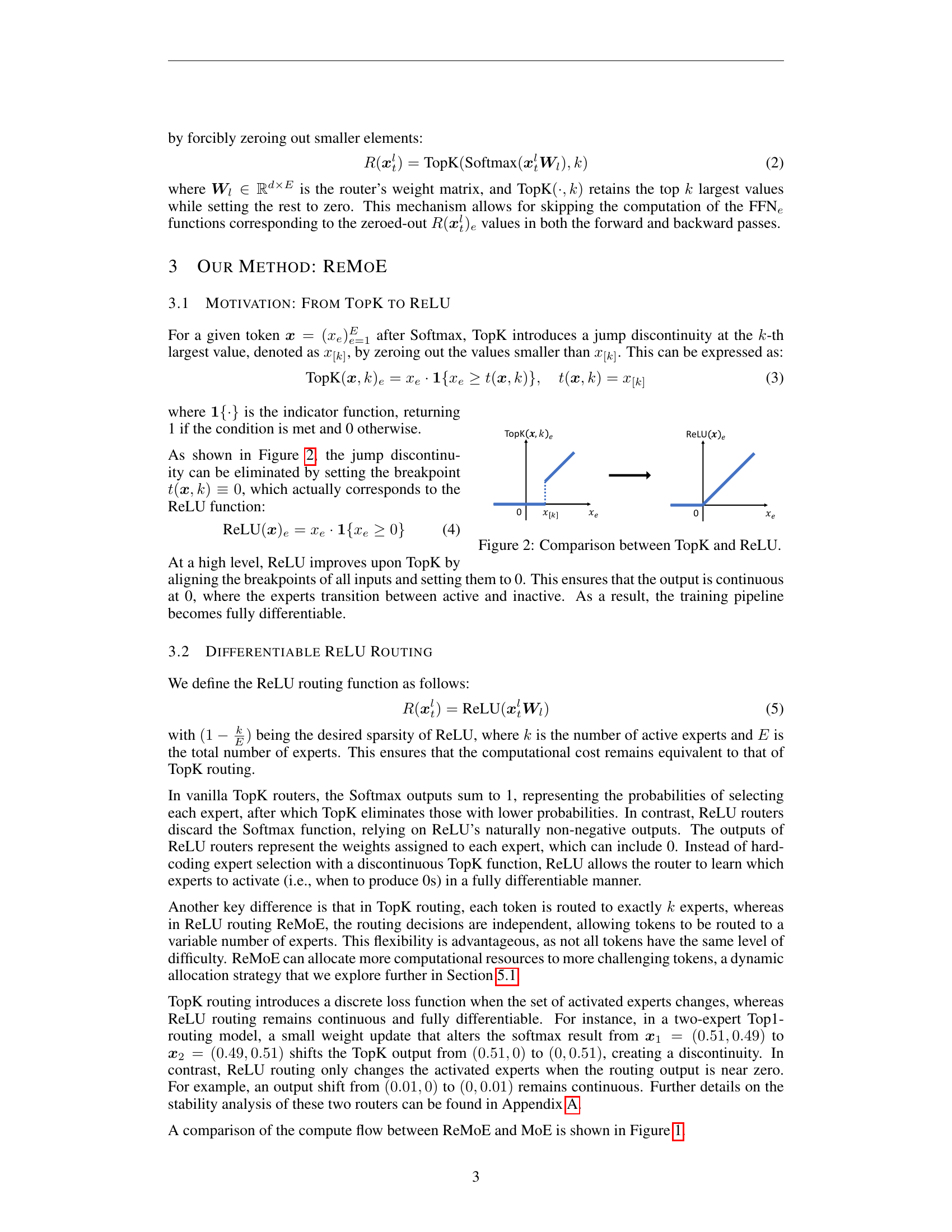
🔼 The figure compares the TopK and ReLU activation functions. The TopK function, commonly used in Mixture-of-Experts (MoE) models, introduces a discontinuity at the k-th largest value by setting all smaller values to zero. This discontinuity creates challenges during model training because it makes the training process non-differentiable at the point of the discontinuity. In contrast, the ReLU function is continuous, and thus differentiable. The figure visually illustrates how the TopK function introduces this abrupt jump (discontinuity), while ReLU remains a continuous smooth function.
read the caption
Figure 2: Comparison between TopK and ReLU.

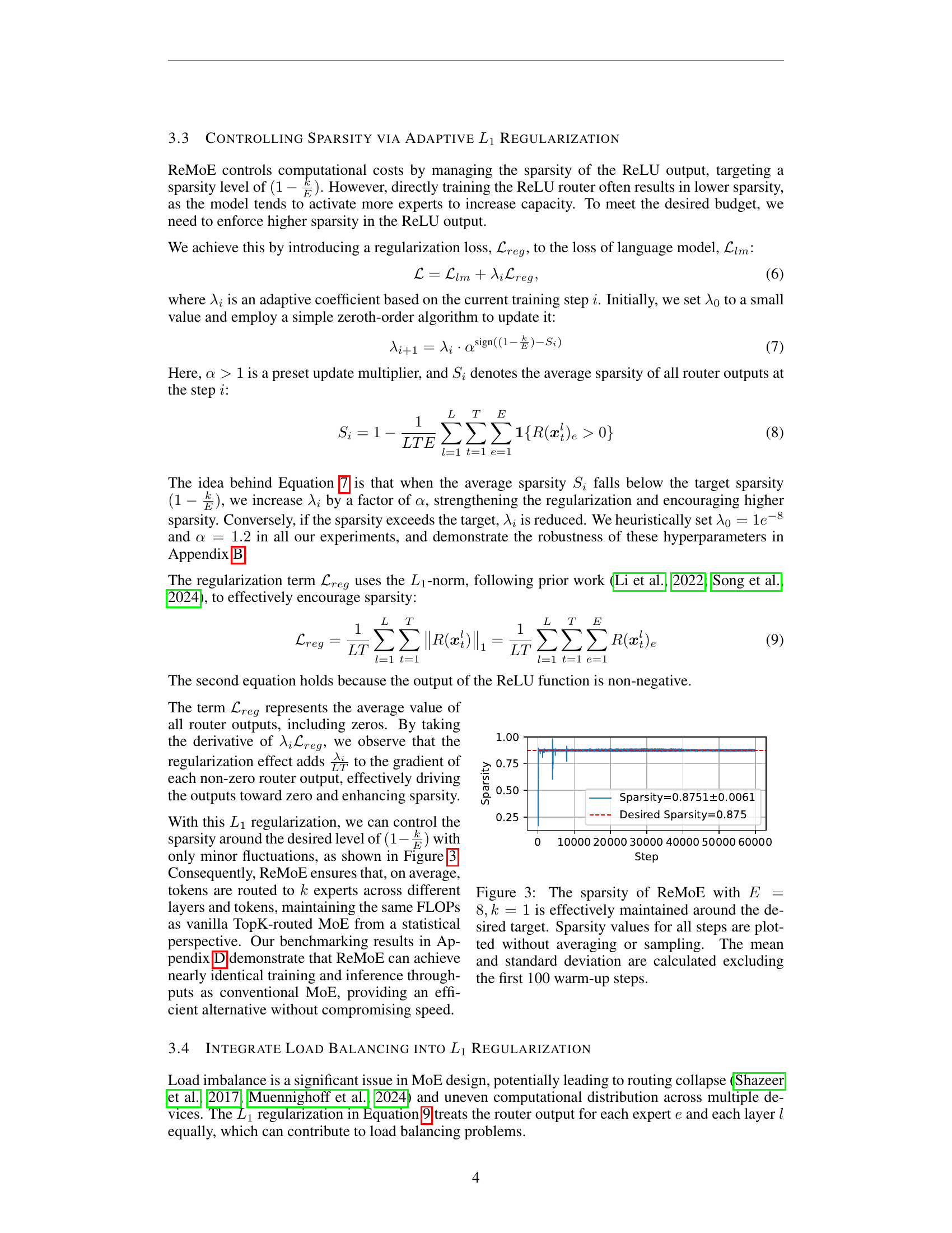
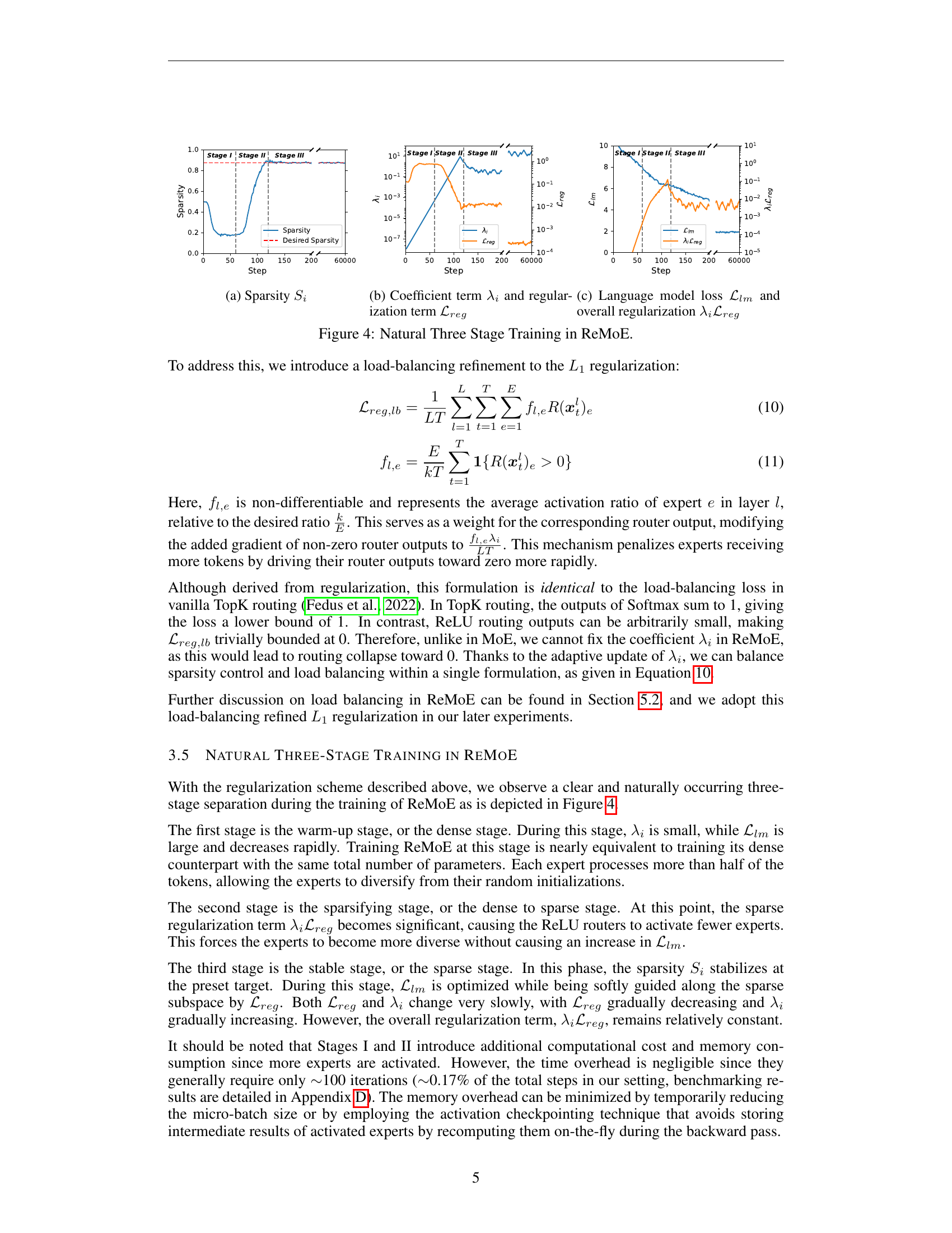
🔼 This figure shows the sparsity of the ReLU Mixture-of-Experts (MoE) model, ReMoE, during training. The model uses 8 experts (E=8) and targets 1 active expert (k=1). The plot displays the sparsity at each training step. No averaging or sampling of the data has been done; all individual data points are plotted. The reported mean and standard deviation for sparsity only take into account the training data after the first 100 steps (a warm-up period), as the model’s behavior during this initial phase is different from its stabilized later performance.
read the caption
Figure 3: The sparsity of ReMoE with E=8,k=1formulae-sequence𝐸8𝑘1E=8,k=1italic_E = 8 , italic_k = 1 is effectively maintained around the desired target. Sparsity values for all steps are plotted without averaging or sampling. The mean and standard deviation are calculated excluding the first 100 warm-up steps.

🔼 This figure displays the sparsity (𝑆𝑖) over training steps. Sparsity is the proportion of inactive router outputs. The adaptive L1 regularization dynamically adjusts sparsity to maintain the desired level. The figure helps to visualize how the adaptive sparsity control method works and how it achieves the desired sparsity level of (1−𝑘/𝐸) during training, where k is the number of active experts and E is the total number of experts.
read the caption
(a) Sparsity Sisubscript𝑆𝑖S_{i}italic_S start_POSTSUBSCRIPT italic_i end_POSTSUBSCRIPT

🔼 The figure shows the trends of the coefficient λ𝑖 and the regularization term ℒ𝑟𝑒𝑔 during the training process. The coefficient λ𝑖 is adaptively adjusted based on the current average sparsity, increasing when sparsity is below the target and decreasing when sparsity is above the target. The regularization term ℒ𝑟𝑒𝑔, which uses the L1 norm, encourages sparsity in the ReLU output, driving the outputs towards zero and thus promoting sparsity in expert activation.
read the caption
(b) Coefficient term λisubscript𝜆𝑖\lambda_{i}italic_λ start_POSTSUBSCRIPT italic_i end_POSTSUBSCRIPT and regularization term ℒregsubscriptℒ𝑟𝑒𝑔\mathcal{L}_{reg}caligraphic_L start_POSTSUBSCRIPT italic_r italic_e italic_g end_POSTSUBSCRIPT

🔼 The figure shows the training curves of the language model loss (ℒlmsubscriptℒ𝑙𝑚) and the overall regularization term (λiℒregsubscript𝜆𝑖subscriptℒ𝑟𝑒𝑔). The language model loss represents the model’s performance on the training data, decreasing as the model learns. The overall regularization term is added to the loss to control the sparsity of the model, enforcing a desired level of sparsity. The regularization loss increases during the training process in the first two stages and plateaus in the final stage, indicating the effectiveness of the regularization technique in achieving the desired sparsity.
read the caption
(c) Language model loss ℒlmsubscriptℒ𝑙𝑚\mathcal{L}_{lm}caligraphic_L start_POSTSUBSCRIPT italic_l italic_m end_POSTSUBSCRIPT and overall regularization λiℒregsubscript𝜆𝑖subscriptℒ𝑟𝑒𝑔\lambda_{i}\mathcal{L}_{reg}italic_λ start_POSTSUBSCRIPT italic_i end_POSTSUBSCRIPT caligraphic_L start_POSTSUBSCRIPT italic_r italic_e italic_g end_POSTSUBSCRIPT

🔼 This figure illustrates the three natural stages of training in the ReMoE model. Stage I is a dense stage where sparsity is low and the language model loss (Llm) decreases rapidly. Stage II is a sparsifying stage where the regularization term (Lreg) becomes significant, driving down the sparsity level towards the target. Finally, Stage III is a sparse stage where sparsity stabilizes around the target value and Llm continues to decrease while the regularization term remains relatively stable. The plot shows the sparsity (Si), the regularization coefficient (λi), the language model loss (Llm), and the overall regularization term (λiLreg) over training steps.
read the caption
Figure 4: Natural Three Stage Training in ReMoE.

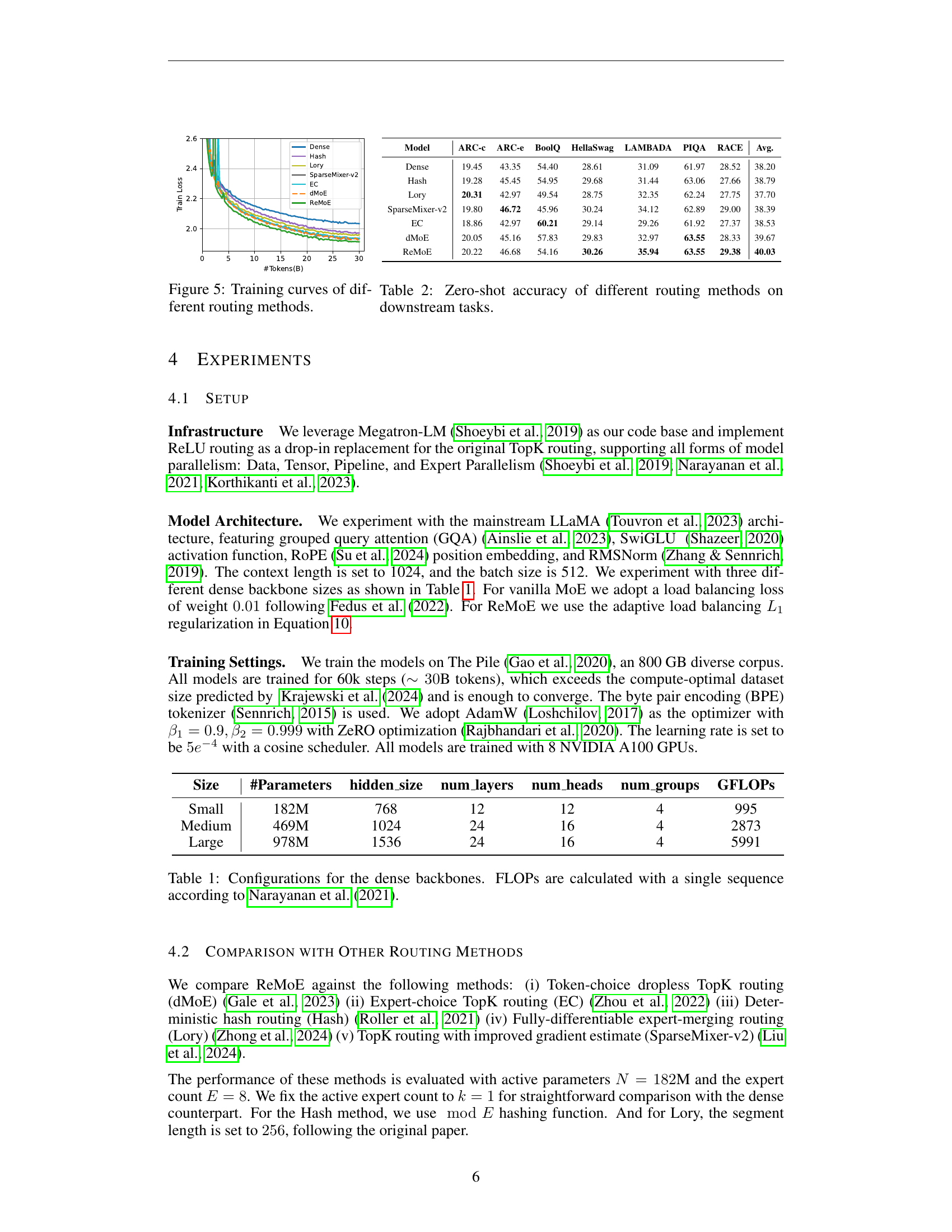
🔼 This figure compares the training curves of various Mixture-of-Experts (MoE) routing methods. The x-axis represents the number of tokens processed during training (in billions), and the y-axis represents the validation loss. Different lines represent different routing methods, allowing for a visual comparison of their convergence rates and final performance. The figure provides insights into the relative training efficiency and stability of each routing approach.
read the caption
Figure 5: Training curves of different routing methods.

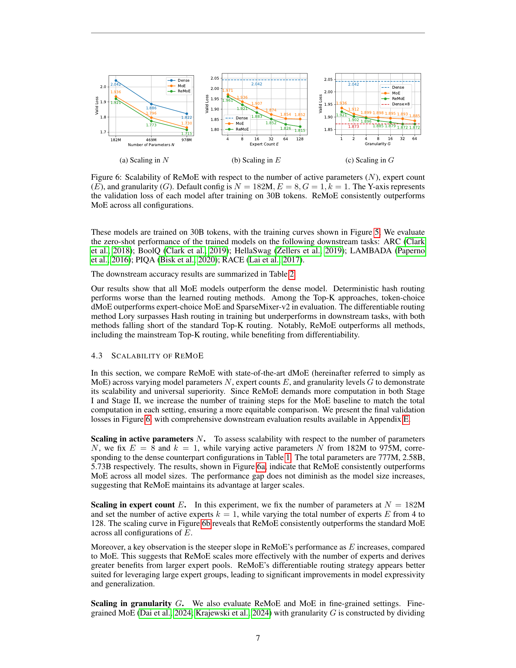
🔼 This figure shows how the validation loss of different models changes with the number of active parameters (N). Three different model sizes are evaluated: 182M, 469M, and 978M parameters. For each model size, the validation loss is plotted for both the ReMoE model and a standard MoE model. The plot demonstrates the performance of ReMoE in comparison to a standard MoE model across different scales of active model parameters.
read the caption
(a) Scaling in N𝑁Nitalic_N

🔼 This figure demonstrates the scalability of ReMoE and MoE models as the number of experts (E) increases. The x-axis represents the number of experts, while the y-axis shows the validation loss achieved after training on 30 billion tokens. The results across various expert counts highlight ReMoE’s consistent superior performance compared to the standard MoE, indicating that ReMoE leverages the increased expert capacity more effectively.
read the caption
(b) Scaling in E𝐸Eitalic_E

🔼 This figure demonstrates the scalability of ReMoE (and MoE for comparison) with respect to granularity (G). Granularity refers to the level of detail or fineness in the model’s expert networks. A higher granularity means that each expert is divided into more specialized sub-experts, allowing for finer-grained control of the model’s capacity. The Y-axis shows the validation loss achieved after training on 30 billion tokens for various granularities. The graph reveals how the model’s performance changes as the granularity increases, highlighting the impact of this hyperparameter on model efficiency and generalization.
read the caption
(c) Scaling in G𝐺Gitalic_G

🔼 This figure displays the scalability of the ReMoE model (and its comparison with the MoE model) across three key aspects: the number of active parameters (N), the number of experts (E), and the granularity (G). Each subplot shows the validation loss achieved after training on 30 billion tokens. The default setting is N=182M, E=8, G=1, and k=1. The results clearly demonstrate that ReMoE consistently outperforms MoE across various configurations and scales.
read the caption
Figure 6: Scalability of ReMoE with respect to the number of active parameters (N𝑁Nitalic_N), expert count (E𝐸Eitalic_E), and granularity (G𝐺Gitalic_G). Default config is N=182M,E=8,G=1,k=1formulae-sequence𝑁182Mformulae-sequence𝐸8formulae-sequence𝐺1𝑘1N=182\text{M},E=8,G=1,k=1italic_N = 182 M , italic_E = 8 , italic_G = 1 , italic_k = 1. The Y-axis represents the validation loss of each model after training on 30B tokens. ReMoE consistently outperforms MoE across all configurations.

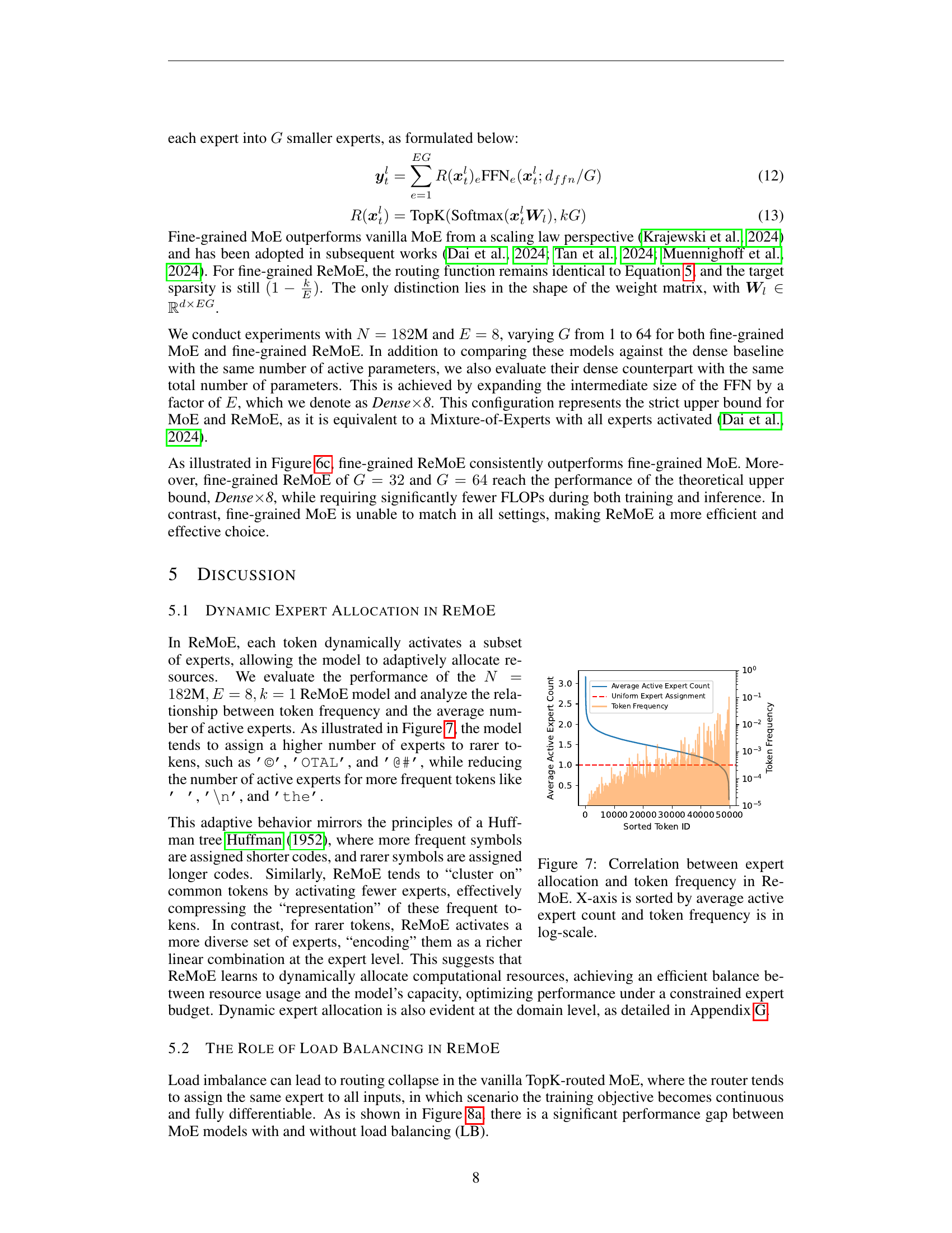
🔼 This figure illustrates the relationship between the frequency of tokens in the input text and the number of experts assigned to those tokens by the ReMoE model. The x-axis is sorted based on the average number of active experts for each token, and the y-axis (token frequency) uses a logarithmic scale to better visualize the wide range of token frequencies. The graph shows that less frequent tokens tend to have more experts assigned to them, implying that the model devotes more computational resources to processing less common words, possibly because they are more ambiguous or carry more crucial contextual information. Conversely, highly frequent tokens (like common function words) usually have fewer experts allocated to them, suggesting a more efficient processing strategy for these well-understood words. This demonstrates ReMoE’s ability to dynamically allocate computational resources based on token significance, optimizing performance.
read the caption
Figure 7: Correlation between expert allocation and token frequency in ReMoE. X-axis is sorted by average active expert count and token frequency is in log-scale.

🔼 This figure compares the training curves of Mixture-of-Experts (MoE) models with and without load balancing, and also includes ReMoE models with and without load balancing. The x-axis represents the number of tokens processed during training, and the y-axis represents the training loss. The curves show how the training loss changes over time for each model. It demonstrates the impact of load balancing on the training process and loss convergence.
read the caption
(a) Training curves of MoE and ReMoE with and without load balancing

🔼 This figure visualizes the average distribution of tokens routed to each expert in ReMoE without load balancing. Each cell represents an expert, and the color intensity indicates the proportion of tokens routed to that expert. A darker shade implies a higher proportion of tokens. White cells represent experts that received very few tokens (less than 1/64 of the total). The figure is valuable for understanding the expert allocation strategy in ReMoE before the load balancing refinement is applied and helps to visualize potential imbalances in expert usage.
read the caption
(b) Average routed tokens ratio of ReMoE w.o. LB

🔼 This figure visualizes the average number of tokens routed to each expert in ReMoE (Mixture-of-Experts with ReLU routing) when load balancing is applied. Each cell represents the average number of tokens routed to a specific expert across all tokens and layers. The color intensity reflects the magnitude of the average, with deeper colors representing a higher average number of tokens. This provides insight into the distribution of computational load across experts and helps to evaluate the effectiveness of the load balancing technique in ensuring a more uniform distribution of computational work among experts.
read the caption
(c) Average routed tokens ratio of ReMoE w. LB

🔼 This figure shows the sparsity of the ReLU router’s output across different layers in the ReMoE model. Sparsity, in this context, refers to the proportion of experts that are not activated (i.e., have zero output) for each layer. The figure illustrates the distribution of sparsity across multiple layers, providing a visualization of how the model dynamically manages the activation of experts during inference. Higher values indicate higher sparsity (more deactivated experts), while lower values indicate lower sparsity (more activated experts). This visualization aids in understanding the model’s behavior and its ability to efficiently allocate computational resources across various layers.
read the caption
(d) Sparsity across different layers in ReMoE

🔼 Figure 8 demonstrates the effects of load balancing on Mixture-of-Experts (MoE) models, comparing the standard MoE with TopK routing and ReMoE with ReLU routing. Subfigure (a) shows the training curves for both models with and without load balancing, highlighting the improved convergence of load-balanced models. Subfigure (b) displays a heatmap visualizing the average number of tokens routed to each expert in each layer for ReMoE, both with and without load balancing. White squares in this heatmap represent inactive experts (those with fewer than 1/64 tokens routed to them). Subfigure (c) shows the average token routing ratios for ReMoE (with and without load balancing) across different layers. Finally, subfigure (d) shows the sparsity in ReMoE models, with and without load balancing, across different layers.
read the caption
Figure 8: Observations on the role of load balancing in MoE and ReMoE. White squares in (b) represent inactive experts with fewer than 1/64 tokens routed to them.
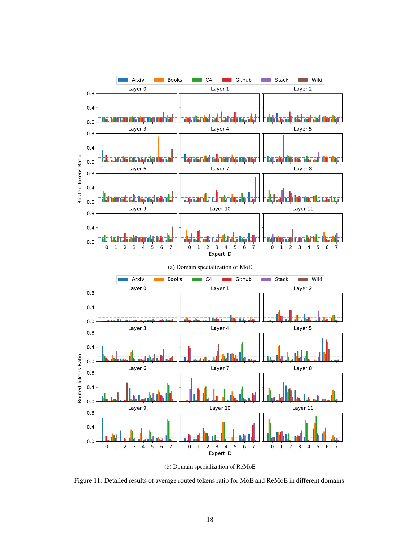
🔼 This figure visualizes the domain specialization of the Mixture-of-Experts (MoE) model. It shows the average proportion of tokens routed to each of the eight experts across twelve layers of the model for six different domains: Arxiv, Books, C4, Github, Stackexchange, and Wikipedia. The bar chart illustrates the degree to which each expert specializes in particular domains, revealing whether experts focus on a single domain or handle multiple domains more generally. A uniform distribution across domains would indicate a lack of specialization, while pronounced differences in the bar heights show a strong domain-specific preference for particular experts.
read the caption
(a) Domain specialization of MoE

🔼 This figure shows the average routed tokens ratio for ReMoE across different domains (Arxiv, Books, C4, Github, Stackexchange, Wiki) and layers (0, 5, and 11). Each bar represents the proportion of tokens assigned to a specific expert within a layer and domain. The figure highlights ReMoE’s domain specialization, where some experts are strongly activated within specific domains, unlike MoE where experts are more uniformly distributed across domains.
read the caption
(b) Domain specialization of ReMoE

🔼 This figure compares the average number of tokens routed to each expert in both MoE and ReMoE models across 12 layers. The models are evaluated across six different domains (Arxiv, Books, C4, Github, StackExchange, Wiki). The gray dashed lines represent a uniform distribution, indicating that each expert would receive an equal number of tokens. The figure demonstrates that the ReMoE model exhibits stronger domain specialization than the standard MoE model, meaning that specific experts tend to handle tokens from particular domains more frequently. This visualization helps illustrate the adaptive resource allocation capabilities of ReMoE.
read the caption
Figure 9: Average routed tokens ratio for MoE and ReMoE across 12 layers and 8 experts in different domains. The gray dashed lines indicate uniform distribution. ReMoE shows stronger domain specialization.

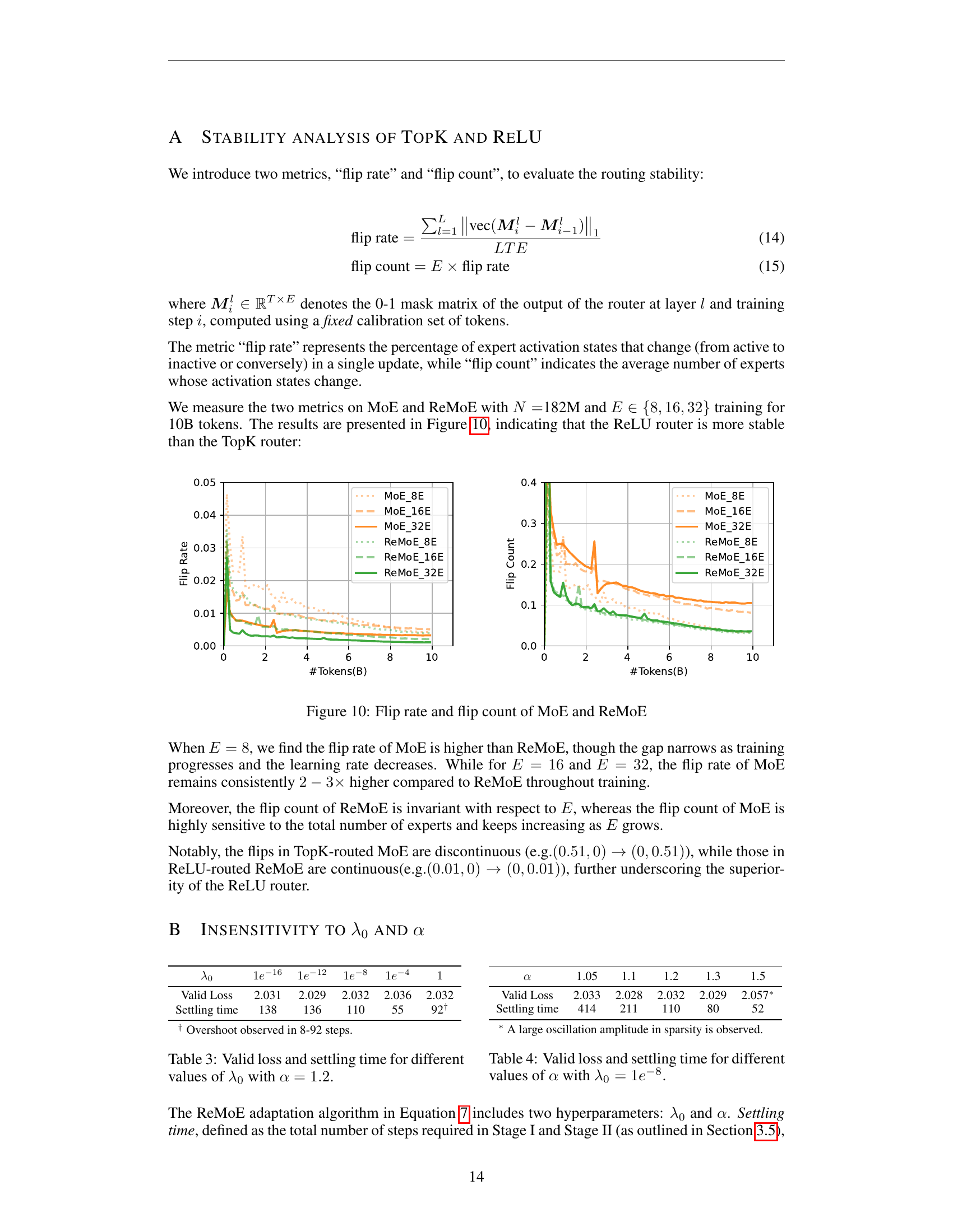
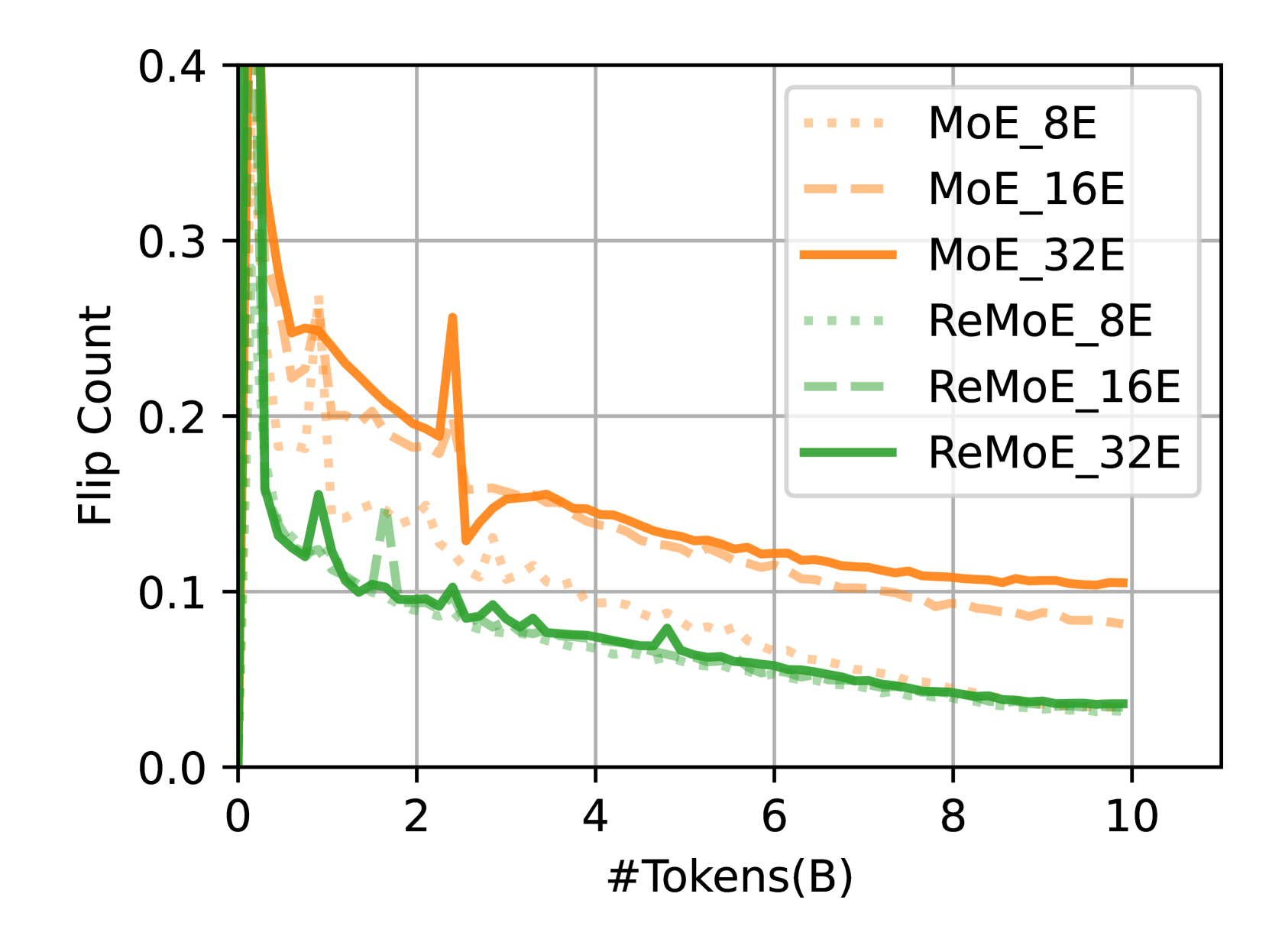
🔼 This figure shows the stability of routing in Mixture-of-Experts (MoE) models using two metrics: ‘flip rate’ and ‘flip count’. The flip rate represents the percentage of expert activation states that change (active to inactive or vice versa) in a single update, while the flip count indicates the average number of experts whose activation states change. The results are presented for MoE and ReMoE models with different numbers of experts (E = 8, 16, 32) trained on 10 billion tokens. The figure demonstrates that ReLU routing in ReMoE is more stable than TopK routing in MoE.
read the caption
Figure 10: Flip rate and flip count of MoE and ReMoE

🔼 This table shows how the performance of the ReMoE model is affected by different values of the hyperparameter λ₀ (lambda-zero), which controls the sparsity of the ReLU router’s output. The experiment uses a fixed value of α (alpha) = 1.2. The table displays the validation loss achieved and the number of training steps it took for the model to reach a stable state (settling time) for various λ₀ values. A low settling time indicates faster convergence.
read the caption
Table 3: Valid loss and settling time for different values of λ0subscript𝜆0\lambda_{0}italic_λ start_POSTSUBSCRIPT 0 end_POSTSUBSCRIPT with α=1.2𝛼1.2\alpha=1.2italic_α = 1.2.
More on tables
| Model | ARC-c | ARC-e | BoolQ | HellaSwag | LAMBADA | PIQA | RACE | Avg. |
|---|---|---|---|---|---|---|---|---|
| Dense | 19.45 | 43.35 | 54.40 | 28.61 | 31.09 | 61.97 | 28.52 | 38.20 |
| Hash | 19.28 | 45.45 | 54.95 | 29.68 | 31.44 | 63.06 | 27.66 | 38.79 |
| Lory | 20.31 | 42.97 | 49.54 | 28.75 | 32.35 | 62.24 | 27.75 | 37.70 |
| SparseMixer-v2 | 19.80 | 46.72 | 45.96 | 30.24 | 34.12 | 62.89 | 29.00 | 38.39 |
| EC | 18.86 | 42.97 | 60.21 | 29.14 | 29.26 | 61.92 | 27.37 | 38.53 |
| dMoE | 20.05 | 45.16 | 57.83 | 29.83 | 32.97 | 63.55 | 28.33 | 39.67 |
| ReMoE | 20.22 | 46.68 | 54.16 | 30.26 | 35.94 | 63.55 | 29.38 | 40.03 |
🔼 This table presents the zero-shot accuracy results of different MoE routing methods on several downstream tasks. Zero-shot accuracy refers to the model’s performance on these tasks without any fine-tuning or task-specific training. The routing methods compared include ReMoE (the proposed method), TopK routing variants (dMoE, EC), deterministic hash routing (Hash), fully-differentiable expert merging routing (Lory), and an improved TopK routing method (SparseMixer-v2). The downstream tasks used for evaluation represent a variety of natural language understanding challenges.
read the caption
Table 2: Zero-shot accuracy of different routing methods on downstream tasks.
| λ₀ | 1e⁻¹⁶ | 1e⁻¹² | 1e⁻⁸ | 1e⁻⁴ | 1 |
|---|---|---|---|---|---|
| Valid Loss | 2.031 | 2.029 | 2.032 | 2.036 | 2.032 |
| Settling time | 138 | 136 | 110 | 55 | 92† |
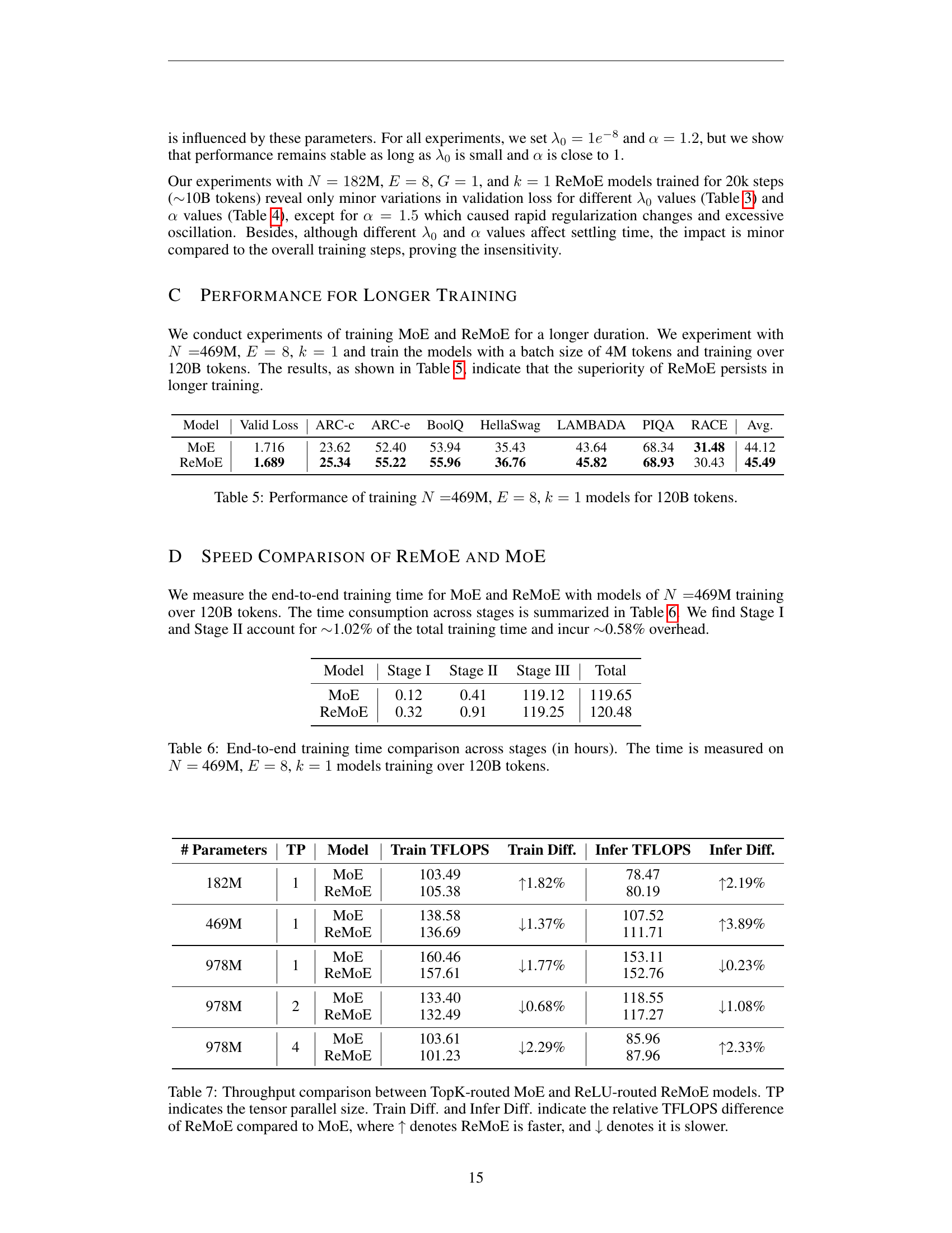
🔼 This table presents the results of training larger language models with 469 million parameters, 8 expert groups, and a sparsity of 1 (meaning only one expert is activated per token) for 120 billion tokens. It shows the performance (measured by validation loss and several downstream task accuracies) of both the standard Mixture of Experts (MoE) model and the proposed ReMoE model after this extensive training regimen. The downstream tasks measure the models’ zero-shot performance on various question answering and text generation benchmarks.
read the caption
Table 5: Performance of training N=𝑁absentN=italic_N =469M, E=8𝐸8E=8italic_E = 8, k=1𝑘1k=1italic_k = 1 models for 120B tokens.
| α | 1.05 | 1.1 | 1.2 | 1.3 | 1.5 |
|---|---|---|---|---|---|
| Valid Loss | 2.033 | 2.028 | 2.032 | 2.029 | 2.057* |
| Settling time | 414 | 211 | 110 | 80 | 52 |
🔼 This table presents a detailed breakdown of the end-to-end training time for both MoE and ReMoE models. The training time is categorized into three stages: Stage I, Stage II, and Stage III. The model used for this comparison has 469 million parameters (N=469M), 8 experts (E=8), and uses only 1 expert at a time (k=1) during the main training phase. The total number of tokens used for training was 120 billion. The table shows the time taken (in hours) for each stage of training, allowing a direct comparison of the efficiency of ReMoE and MoE across different training phases.
read the caption
Table 6: End-to-end training time comparison across stages (in hours). The time is measured on N=𝑁absentN=italic_N = 469M, E=8𝐸8E=8italic_E = 8, k=1𝑘1k=1italic_k = 1 models training over 120B tokens.
| Model | Valid Loss | ARC-c | ARC-e | BoolQ | HellaSwag | LAMBADA | PIQA | RACE | Avg. |
|---|---|---|---|---|---|---|---|---|---|
| MoE | 1.716 | 23.62 | 52.40 | 53.94 | 35.43 | 43.64 | 68.34 | 31.48 | 44.12 |
| ReMoE | 1.689 | 25.34 | 55.22 | 55.96 | 36.76 | 45.82 | 68.93 | 30.43 | 45.49 |
🔼 This table compares the training and inference throughput of ReMoE (ReLU routing) against TopK-routed MoE for different model sizes and levels of tensor parallelism. It shows the training and inference TFLOPS (TeraFLOPS) for each model, and calculates the percentage difference in throughput between ReMoE and MoE. A positive percentage indicates ReMoE is faster, and a negative percentage shows ReMoE is slower. The table helps demonstrate the computational efficiency of ReMoE relative to a standard MoE model, showing that ReMoE achieves comparable performance without significant speed penalties.
read the caption
Table 7: Throughput comparison between TopK-routed MoE and ReLU-routed ReMoE models. TP indicates the tensor parallel size. Train Diff. and Infer Diff. indicate the relative TFLOPS difference of ReMoE compared to MoE, where ↑ denotes ReMoE is faster, and ↓ denotes it is slower.
| Model | Stage I | Stage II | Stage III | Total |
|---|---|---|---|---|
| MoE | 0.12 | 0.41 | 119.12 | 119.65 |
| ReMoE | 0.32 | 0.91 | 119.25 | 120.48 |
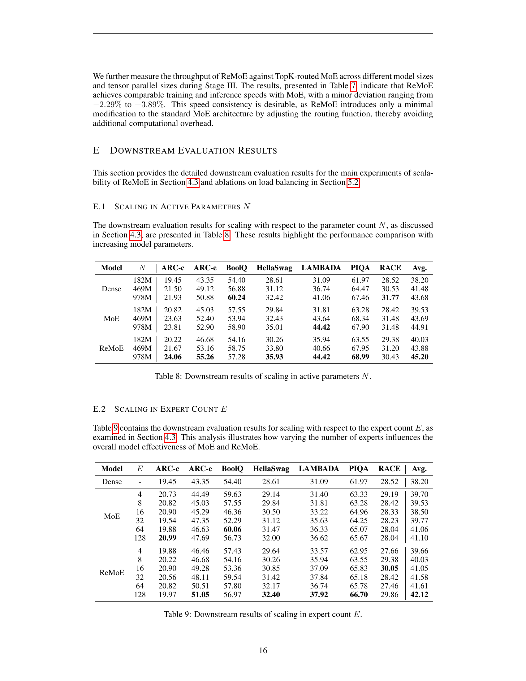
🔼 This table presents the downstream task evaluation results for the scaling experiments with respect to the number of active parameters (N). It compares the performance of different models (Dense, MoE, and ReMoE) across three different sizes of models (182M, 469M, and 978M parameters). The results show the zero-shot accuracy on various downstream tasks (ARC-c, ARC-e, BoolQ, HellaSwag, LAMBADA, PIQA, RACE) for each model and size. This allows for an assessment of how model performance scales with increasing model size and the relative performance of the different models.
read the caption
Table 8: Downstream results of scaling in active parameters N𝑁Nitalic_N.
| # Parameters | TP | Model | Train TFLOPS | Train Diff. | Infer TFLOPS | Infer Diff. |
|---|---|---|---|---|---|---|
| 182M | 1 | MoE | 103.49 | ↑1.82% | 78.47 | ↑2.19% |
| ReMoE | 105.38 | 80.19 | ||||
| 469M | 1 | MoE | 138.58 | ↓1.37% | 107.52 | ↑3.89% |
| ReMoE | 136.69 | 111.71 | ||||
| 978M | 1 | MoE | 160.46 | ↓1.77% | 153.11 | ↓0.23% |
| ReMoE | 157.61 | 152.76 | ||||
| 978M | 2 | MoE | 133.40 | ↓0.68% | 118.55 | ↓1.08% |
| ReMoE | 132.49 | 117.27 | ||||
| 978M | 4 | MoE | 103.61 | ↓2.29% | 85.96 | ↑2.33% |
| ReMoE | 101.23 | 87.96 |
🔼 This table presents the downstream task performance results for scaling experiments with respect to the number of experts (E). It shows how changing the expert count affects the overall model’s effectiveness across various downstream tasks. The results are compared between the standard Mixture-of-Experts (MoE) and the proposed ReMoE models. It allows for analyzing the scalability and performance trade-offs of increasing the number of experts in the MoE architecture.
read the caption
Table 9: Downstream results of scaling in expert count E𝐸Eitalic_E.
| Model | N | ARC-c | ARC-e | BoolQ | HellaSwag | LAMBADA | PIQA | RACE | Avg. |
|---|---|---|---|---|---|---|---|---|---|
| Dense | 182M | 19.45 | 43.35 | 54.40 | 28.61 | 31.09 | 61.97 | 28.52 | 38.20 |
| 469M | 21.50 | 49.12 | 56.88 | 31.12 | 36.74 | 64.47 | 30.53 | 41.48 | |
| 978M | 21.93 | 50.88 | 60.24 | 32.42 | 41.06 | 67.46 | 31.77 | 43.68 | |
| MoE | 182M | 20.82 | 45.03 | 57.55 | 29.84 | 31.81 | 63.28 | 28.42 | 39.53 |
| 469M | 23.63 | 52.40 | 53.94 | 32.43 | 43.64 | 68.34 | 31.48 | 43.69 | |
| 978M | 23.81 | 52.90 | 58.90 | 35.01 | 44.42 | 67.90 | 31.48 | 44.91 | |
| ReMoE | 182M | 20.22 | 46.68 | 54.16 | 30.26 | 35.94 | 63.55 | 29.38 | 40.03 |
| 469M | 21.67 | 53.16 | 58.75 | 33.80 | 40.66 | 67.95 | 31.20 | 43.88 | |
| 978M | 24.06 | 55.26 | 57.28 | 35.93 | 44.42 | 68.99 | 30.43 | 45.20 |
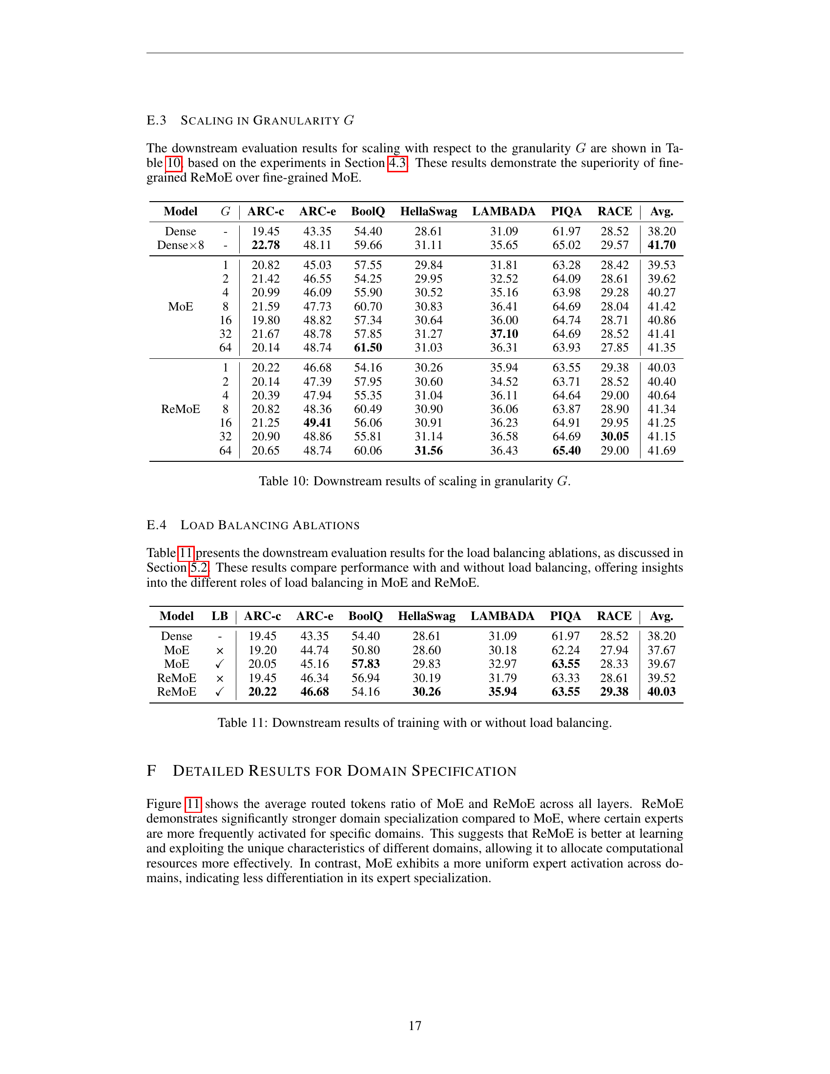
🔼 This table presents the results of experiments evaluating the impact of granularity (G) on model performance. Granularity refers to the level of detail or refinement in the model’s expert modules. The table compares the performance of different models (Dense, MoE, and ReMoE) across various granularities. The results include downstream task accuracy (ARC-c, ARC-e, BoolQ, HellaSwag, LAMBADA, PIQA, RACE, and Avg.) for each model and granularity level. This allows assessing how the model’s performance changes as the granularity (and thus the model’s complexity and capacity) varies.
read the caption
Table 10: Downstream results of scaling in granularity G𝐺Gitalic_G.
| Model | E | ARC-c | ARC-e | BoolQ | HellaSwag | LAMBADA | PIQA | RACE | Avg. |
|---|---|---|---|---|---|---|---|---|---|
| Dense | - | 19.45 | 43.35 | 54.40 | 28.61 | 31.09 | 61.97 | 28.52 | 38.20 |
| MoE | |||||||||
| 4 | 20.73 | 44.49 | 59.63 | 29.14 | 31.40 | 63.33 | 29.19 | 39.70 | |
| 8 | 20.82 | 45.03 | 57.55 | 29.84 | 31.81 | 63.28 | 28.42 | 39.53 | |
| 16 | 20.90 | 45.29 | 46.36 | 30.50 | 33.22 | 64.96 | 28.33 | 38.50 | |
| 32 | 19.54 | 47.35 | 52.29 | 31.12 | 35.63 | 64.25 | 28.23 | 39.77 | |
| 64 | 19.88 | 46.63 | 60.06 | 31.47 | 36.33 | 65.07 | 28.04 | 41.06 | |
| 128 | 20.99 | 47.69 | 56.73 | 32.00 | 36.62 | 65.67 | 28.04 | 41.10 | |
| ReMoE | |||||||||
| 4 | 19.88 | 46.46 | 57.43 | 29.64 | 33.57 | 62.95 | 27.66 | 39.66 | |
| 8 | 20.22 | 46.68 | 54.16 | 30.26 | 35.94 | 63.55 | 29.38 | 40.03 | |
| 16 | 20.90 | 49.28 | 53.36 | 30.85 | 37.09 | 65.83 | 30.05 | 41.05 | |
| 32 | 20.56 | 48.11 | 59.54 | 31.42 | 37.84 | 65.18 | 28.42 | 41.58 | |
| 64 | 20.82 | 50.51 | 57.80 | 32.17 | 36.74 | 65.78 | 27.46 | 41.61 | |
| 128 | 19.97 | 51.05 | 56.97 | 32.40 | 37.92 | 66.70 | 29.86 | 42.12 |
🔼 This table presents the downstream task evaluation results for models trained with and without load balancing. It compares the performance of MoE and ReMoE models on various downstream tasks, highlighting the impact of load balancing on overall model accuracy. The results help to understand the contribution of load balancing to the performance differences between MoE and ReMoE.
read the caption
Table 11: Downstream results of training with or without load balancing.
| Model | G | ARC-c | ARC-e | BoolQ | HellaSwag | LAMBADA | PIQA | RACE | Avg. |
|---|---|---|---|---|---|---|---|---|---|
| Dense | - | 19.45 | 43.35 | 54.40 | 28.61 | 31.09 | 61.97 | 28.52 | 38.20 |
| Dense × 8 | - | 22.78 | 48.11 | 59.66 | 31.11 | 35.65 | 65.02 | 29.57 | 41.70 |
| MoE 1 | 1 | 20.82 | 45.03 | 57.55 | 29.84 | 31.81 | 63.28 | 28.42 | 39.53 |
| MoE 2 | 2 | 21.42 | 46.55 | 54.25 | 29.95 | 32.52 | 64.09 | 28.61 | 39.62 |
| MoE 4 | 4 | 20.99 | 46.09 | 55.90 | 30.52 | 35.16 | 63.98 | 29.28 | 40.27 |
| MoE 8 | 8 | 21.59 | 47.73 | 60.70 | 30.83 | 36.41 | 64.69 | 28.04 | 41.42 |
| MoE 16 | 16 | 19.80 | 48.82 | 57.34 | 30.64 | 36.00 | 64.74 | 28.71 | 40.86 |
| MoE 32 | 32 | 21.67 | 48.78 | 57.85 | 31.27 | 37.10 | 64.69 | 28.52 | 41.41 |
| MoE 64 | 64 | 20.14 | 48.74 | 61.50 | 31.03 | 36.31 | 63.93 | 27.85 | 41.35 |
| ReMoE 1 | 1 | 20.22 | 46.68 | 54.16 | 30.26 | 35.94 | 63.55 | 29.38 | 40.03 |
| ReMoE 2 | 2 | 20.14 | 47.39 | 57.95 | 30.60 | 34.52 | 63.71 | 28.52 | 40.40 |
| ReMoE 4 | 4 | 20.39 | 47.94 | 55.35 | 31.04 | 36.11 | 64.64 | 29.00 | 40.64 |
| ReMoE 8 | 8 | 20.82 | 48.36 | 60.49 | 30.90 | 36.06 | 63.87 | 28.90 | 41.34 |
| ReMoE 16 | 16 | 21.25 | 49.41 | 56.06 | 30.91 | 36.23 | 64.91 | 29.95 | 41.25 |
| ReMoE 32 | 32 | 20.90 | 48.86 | 55.81 | 31.14 | 36.58 | 64.69 | 30.05 | 41.15 |
| ReMoE 64 | 64 | 20.65 | 48.74 | 60.06 | 31.56 | 36.43 | 65.40 | 29.00 | 41.69 |
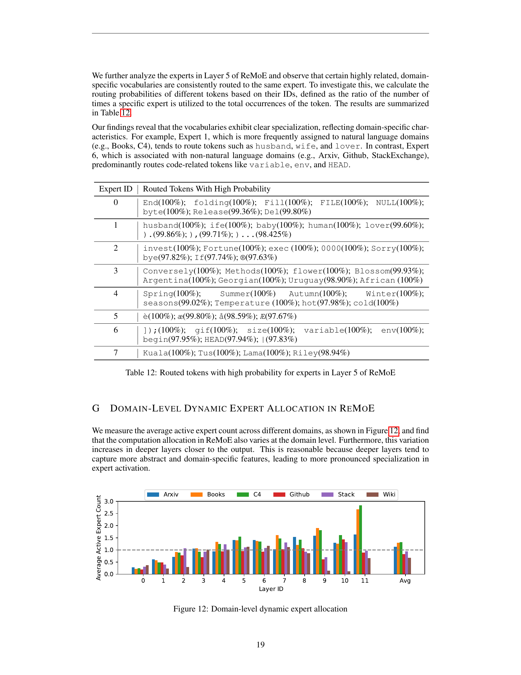
🔼 This table shows tokens with high routing probability to each expert in layer 5 of the ReMoE model. High probability indicates that a given token is frequently routed to a particular expert, suggesting a degree of specialization. The table demonstrates that different experts in ReMoE exhibit a preference for specific types of tokens. For example, some experts show a strong preference for words commonly found in natural language texts (like ‘husband’, ‘wife’, ‘baby’), while others favor technical terms or code-related words (like ‘variable’, ’env’, ‘HEAD’). This specialization highlights how ReMoE learns to dynamically allocate tokens to experts based on their characteristics.
read the caption
Table 12: Routed tokens with high probability for experts in Layer 5 of ReMoE
| Model | LB | ARC-c | ARC-e | BoolQ | HellaSwag | LAMBADA | PIQA | RACE | Avg. |
|---|---|---|---|---|---|---|---|---|---|
| Dense | - | 19.45 | 43.35 | 54.40 | 28.61 | 31.09 | 61.97 | 28.52 | 38.20 |
| MoE | × | 19.20 | 44.74 | 50.80 | 28.60 | 30.18 | 62.24 | 27.94 | 37.67 |
| MoE | ✓ | 20.05 | 45.16 | 57.83 | 29.83 | 32.97 | 63.55 | 28.33 | 39.67 |
| ReMoE | × | 19.45 | 46.34 | 56.94 | 30.19 | 31.79 | 63.33 | 28.61 | 39.52 |
| ReMoE | ✓ | 20.22 | 46.68 | 54.16 | 30.26 | 35.94 | 63.55 | 29.38 | 40.03 |
🔼 This table compares the performance of three different models: the standard Mixture-of-Experts (MoE) model, an MoE model with a near-dense warmup phase added, and the ReMoE model. The near-dense warmup phase for MoE involves initially training with more experts active than usual to improve initial model parameters before transitioning to a sparser training configuration. The table shows the validation loss and downstream task accuracy (across several tasks) for each model to demonstrate the impact of this near-dense warmup strategy on overall performance, particularly in comparison to ReMoE which naturally employs this type of training.
read the caption
Table 13: Performance of MoE with near-dense warmup
| Expert ID | Routed Tokens With High Probability |
|---|---|
| 0 | End(100%); folding(100%); Fill(100%); FILE(100%); NULL(100%); byte(100%); Release(99.36%); Del(99.80%) |
| 1 | husband(100%); ife(100%); baby(100%); human(100%); lover(99.60%); ).(99.86%); ),(99.71%); )...(98.425%) |
| 2 | invest(100%); Fortune(100%); exec (100%); 0000(100%); Sorry(100%); bye(97.82%); If(97.74%); ®(97.63%) |
| 3 | Conversely(100%); Methods(100%); flower(100%); Blossom(99.93%); Argentina(100%); Georgian(100%); Uruguay(98.90%); African (100%) |
| 4 | Spring(100%); Summer(100%) Autumn(100%); Winter(100%); seasons(99.02%); Temperature (100%); hot(97.98%); cold(100%) |
| 5 | è(100%); æ(99.80%); å(98.59%); Æ(97.67%) |
| 6 | ]);(100%); gif(100%); size(100%); variable(100%); env(100%); begin(97.95%); HEAD(97.94%); ` |
| 7 | Kuala(100%); Tus(100%); Lama(100%); Riley(98.94%) |
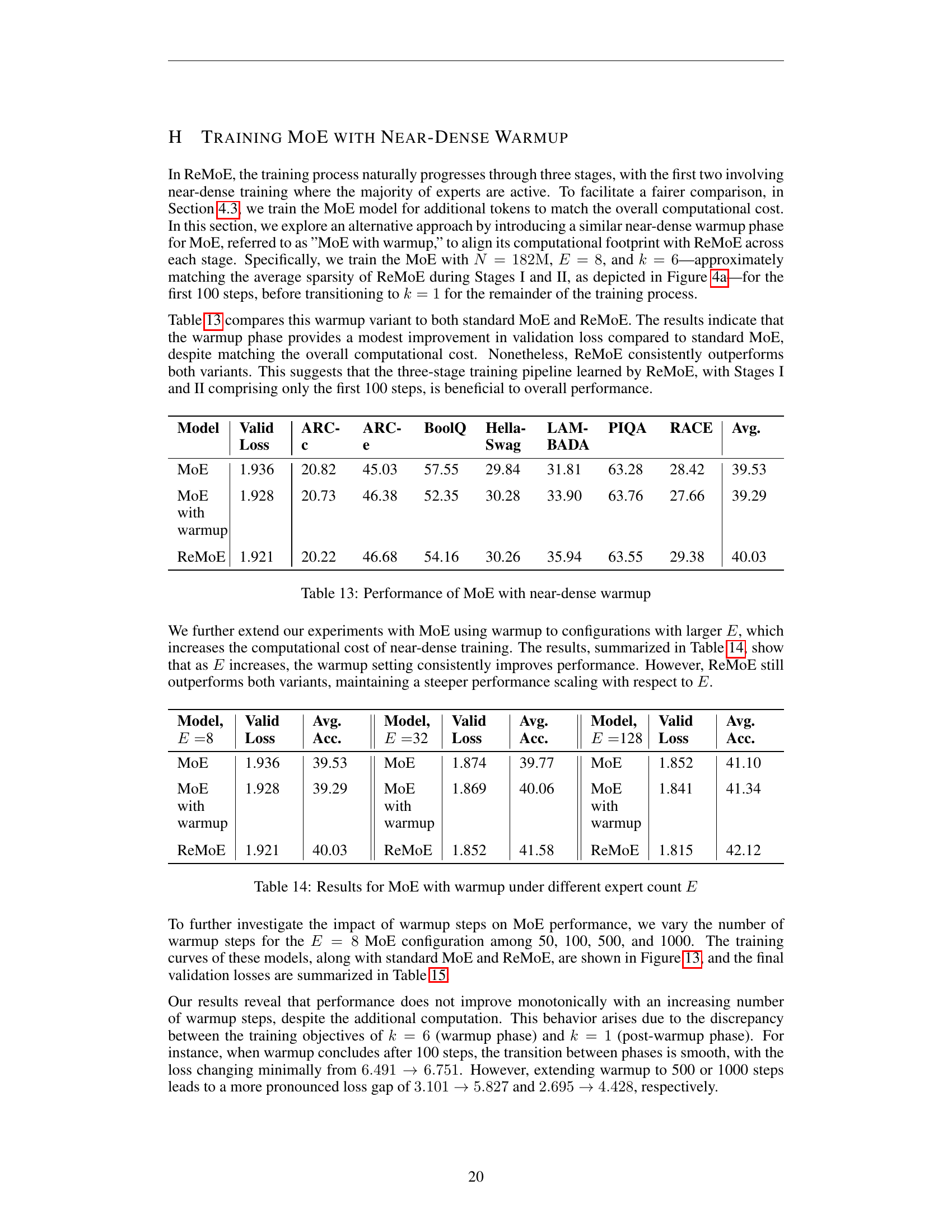
🔼 This table presents the results of experiments comparing the performance of the Mixture-of-Experts (MoE) model with a near-dense warmup phase to the standard MoE and ReMoE models. The near-dense warmup involves training MoE with a larger number of active experts initially (k=6), before transitioning to k=1 for the rest of training. The table shows the validation loss and average accuracy for MoE with and without the warmup phase across different numbers of experts (E=8, E=32, and E=128), highlighting how the warmup strategy impacts performance, particularly as the number of experts increases. ReMoE serves as the baseline for comparison, illustrating its relative performance.
read the caption
Table 14: Results for MoE with warmup under different expert count E𝐸Eitalic_E
| Model | Valid Loss | ARC-c | ARC-e | BoolQ | Hella-Swag | LAM-BADA | PIQA | RACE | Avg. |
|---|---|---|---|---|---|---|---|---|---|
| MoE | 1.936 | 20.82 | 45.03 | 57.55 | 29.84 | 31.81 | 63.28 | 28.42 | 39.53 |
| MoE with warmup | 1.928 | 20.73 | 46.38 | 52.35 | 30.28 | 33.90 | 63.76 | 27.66 | 39.29 |
| ReMoE | 1.921 | 20.22 | 46.68 | 54.16 | 30.26 | 35.94 | 63.55 | 29.38 | 40.03 |
🔼 This table presents the final validation loss achieved by the MoE model (Mixture of Experts) after training with varying numbers of warmup steps. The warmup phase involves initially training the model with a higher number of active experts, gradually transitioning to a sparser configuration. The results show the impact of different warmup lengths on the model’s final performance, highlighting the trade-off between initialization and overall convergence.
read the caption
Table 15: Final validation loss of MoE with different warmup steps
Full paper#
