↗ arXiv ↗ Hugging Face ↗ Papers with Code
TL;DR#
Autoregressive models excel at visual generation but are slow due to their sequential nature. This paper addresses this limitation. Current methods generate images token by token, a process that is inherently slow. Also, prior attempts at parallel generation often sacrifice image quality or require complex model modifications.
This work introduces a novel approach that parallelizes the image generation process by identifying and generating weakly dependent tokens in parallel, while maintaining sequential generation for strongly dependent tokens. The method is simple to implement, requiring no changes to model architecture or tokenizer. Experimental results demonstrate impressive speedups (3.6x-9.5x) with minimal quality loss on ImageNet and UCF-101 datasets, showcasing the practicality of the proposed method.
Key Takeaways#
Why does it matter?#
This paper is crucial because it significantly accelerates autoregressive visual generation, a critical area in computer vision. The method’s simplicity and effectiveness make it broadly applicable, opening new avenues for research in efficient and scalable visual models, and potentially impacting various downstream applications. By tackling the speed limitations of current methods, this work enables the practical application of autoregressive models to more demanding visual tasks such as high-resolution image and video generation. The findings inspire future work on improving generation efficiency without sacrificing quality.
Visual Insights#

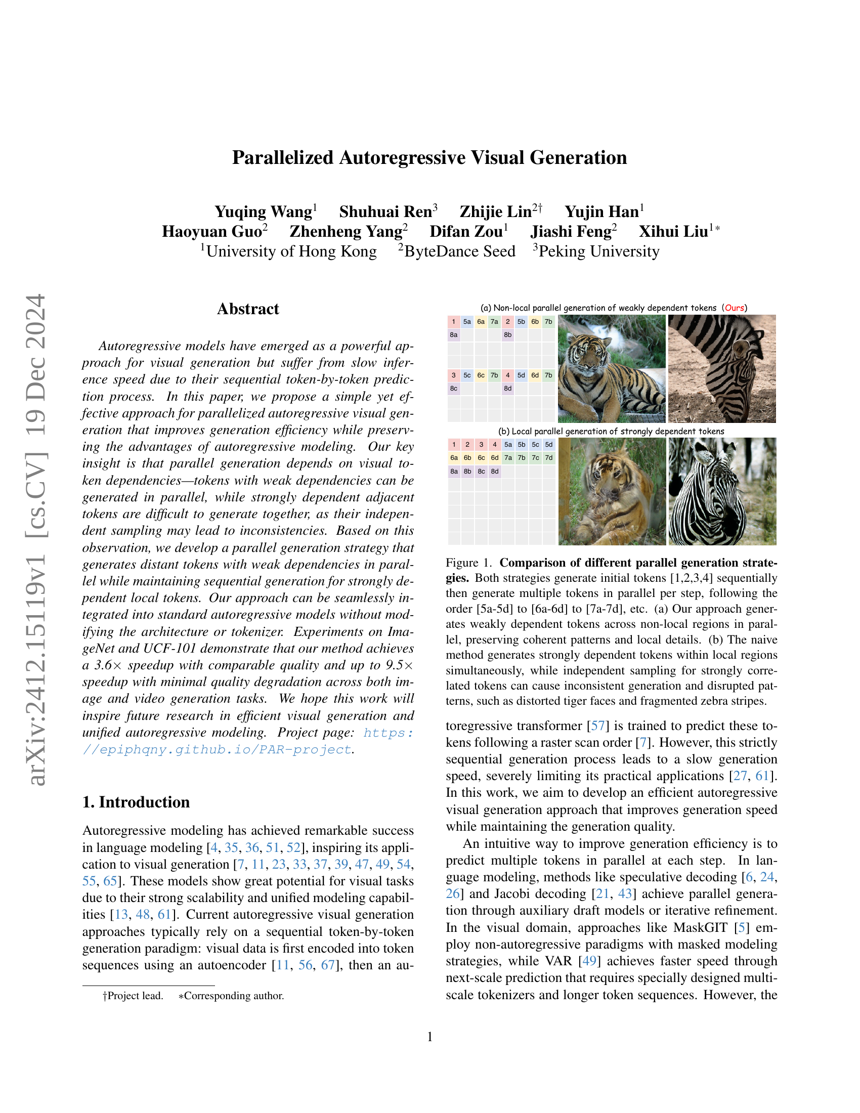
🔼 Figure 1 illustrates two different parallel generation strategies for autoregressive visual models. Both methods start by generating the first four tokens sequentially. Then, they proceed in parallel, generating groups of tokens in a specific order ([5a-5d], [6a-6d], etc.). The key difference lies in the selection of tokens for parallel processing. (a) shows the proposed approach, where weakly dependent tokens from non-adjacent spatial regions are processed concurrently, preserving image coherence and detail. (b) shows a naive approach, which processes strongly dependent tokens from the same region in parallel. In this case, independent sampling can lead to inconsistencies and visual artifacts, as evidenced by the distorted tiger face and fragmented zebra stripes shown in the figure.
read the caption
Figure 1: Comparison of different parallel generation strategies. Both strategies generate initial tokens [1,2,3,4] sequentially then generate multiple tokens in parallel per step, following the order [5a-5d] to [6a-6d] to [7a-7d], etc. (a) Our approach generates weakly dependent tokens across non-local regions in parallel, preserving coherent patterns and local details. (b) The naive method generates strongly dependent tokens within local regions simultaneously, while independent sampling for strongly correlated tokens can cause inconsistent generation and disrupted patterns, such as distorted tiger faces and fragmented zebra stripes.
| Model | Params | Layers | Hidden | Heads |
|---|---|---|---|---|
| PAR-L | 343M | 24 | 1024 | 16 |
| PAR-XL | 775M | 36 | 1280 | 20 |
| PAR-XXL | 1.4B | 48 | 1536 | 24 |
| PAR-3B | 3.1B | 24 | 3200 | 32 |
🔼 This table presents the different model sizes used in the experiments, along with their corresponding architectural configurations. It shows the number of parameters, the number of layers, the hidden dimension, and the number of attention heads for each model variant (PAR-L, PAR-XL, PAR-XXL, PAR-3B). The architectures build upon prior work, as indicated by the citations, demonstrating consistency in design choices across related studies.
read the caption
Table 1: Model sizes and architecture configurations of PAR. The configurations are following previous works [36, 51, 32, 47].
In-depth insights#
Parallel Autoregressive#
The concept of “Parallel Autoregressive” in visual generation aims to address the inherent sequential bottleneck of autoregressive models. Traditional autoregressive models process tokens one by one, resulting in slow inference. A parallel approach seeks to overcome this limitation by identifying and generating independent or weakly dependent tokens concurrently. The core challenge lies in managing dependencies between tokens. Strong dependencies require sequential processing to avoid inconsistencies, while weak dependencies allow for parallelization to speed up generation. A successful parallel autoregressive model must cleverly balance these two aspects. This involves sophisticated token grouping strategies, potentially leveraging spatial information to identify weakly dependent tokens in images or videos. Efficient algorithms for identifying these dependencies are crucial for effective parallelization. The resulting speed-up in inference is significant, offering faster visual generation without substantial quality loss, making the approach highly valuable for practical applications. However, challenges remain in optimizing the trade-off between parallelization and maintaining the quality of autoregressive generation. Further research is needed to explore more robust dependency detection methods and to enhance the compatibility with various autoregressive architectures.
Token Dependency#
The concept of ‘Token Dependency’ is central to efficient autoregressive visual generation. The core idea is that tokens with strong dependencies require sequential generation, mimicking the way humans process visual information. Adjacent tokens, due to their spatial and semantic proximity, exhibit high interdependence, making parallel generation prone to inconsistencies. Weakly dependent tokens, however, can be safely generated in parallel, dramatically speeding up inference without significant quality loss. This dependency is not solely determined by adjacency; spatially distant tokens might have weaker relationships than close neighbors, allowing for strategic grouping and parallel processing. The challenge lies in identifying these dependencies accurately to maximize parallelisation while preserving the coherence of the generated image. Algorithms must effectively partition the visual tokens into groups that balance strong local dependency preservation with opportunities for parallel computation, thereby achieving a balance between computational efficiency and fidelity of generated content.
Non-local Parallelism#
Non-local parallelism, in the context of autoregressive visual generation, offers a compelling approach to accelerate the traditionally slow, sequential process. The core idea revolves around identifying and exploiting weak dependencies between distant image tokens. Unlike naive parallel methods that attempt simultaneous generation of strongly dependent neighboring tokens, leading to inconsistencies, non-local parallelism focuses on generating independent tokens concurrently. This is crucial because independent sampling, a cornerstone of autoregressive models, becomes problematic with strongly correlated tokens, resulting in artifacts and reduced quality. By parallelizing the generation of weakly-dependent, spatially-distant tokens, the overall generation speed significantly increases while maintaining the benefits of autoregressive modeling. Initial tokens, however, require sequential generation to establish global image structure. This strategy strikes a balance between efficiency and quality, showcasing a practical way to enhance autoregressive visual generation without fundamental architectural changes or the introduction of auxiliary models.
Ablation Studies#
Ablation studies systematically remove components of a model to understand their individual contributions. In the context of this research, ablation studies would likely investigate the impact of key design choices on the model’s performance. This could include removing or altering the initial sequential token generation phase, assessing the effect of different attention patterns (e.g., causal vs. full attention), and exploring the influence of varying numbers of parallel tokens generated at each step. Results would highlight the importance of each component and provide insights into the trade-offs between speed and accuracy. For instance, removing the sequential initialization might lead to less coherent results, while restricting attention mechanisms could hurt performance. Such experiments would demonstrate the synergy of the model’s design elements and justify the specific choices made in achieving both high quality and faster generation speed. Ultimately, the ablation study validates the proposed architecture and offers practical recommendations for future model improvements.
Future Directions#
Future research could explore several promising avenues. Improving the parallel generation strategy is crucial; investigating more sophisticated methods for identifying weakly dependent tokens and optimizing the token grouping process could lead to even greater speedups. Exploring different tokenization techniques is another area of interest, potentially enhancing compatibility with various model architectures and visual modalities. Extending the method to other generative tasks, such as high-resolution image generation or 3D visual generation, would broaden its impact. Addressing the trade-off between speed and quality by incorporating more advanced training techniques or using larger model capacities remains a key challenge. Finally, unifying autoregressive and non-autoregressive models into a single framework could lead to a robust hybrid approach that combines the benefits of both paradigms, creating a powerful and flexible tool for visual content generation.
More visual insights#
More on figures

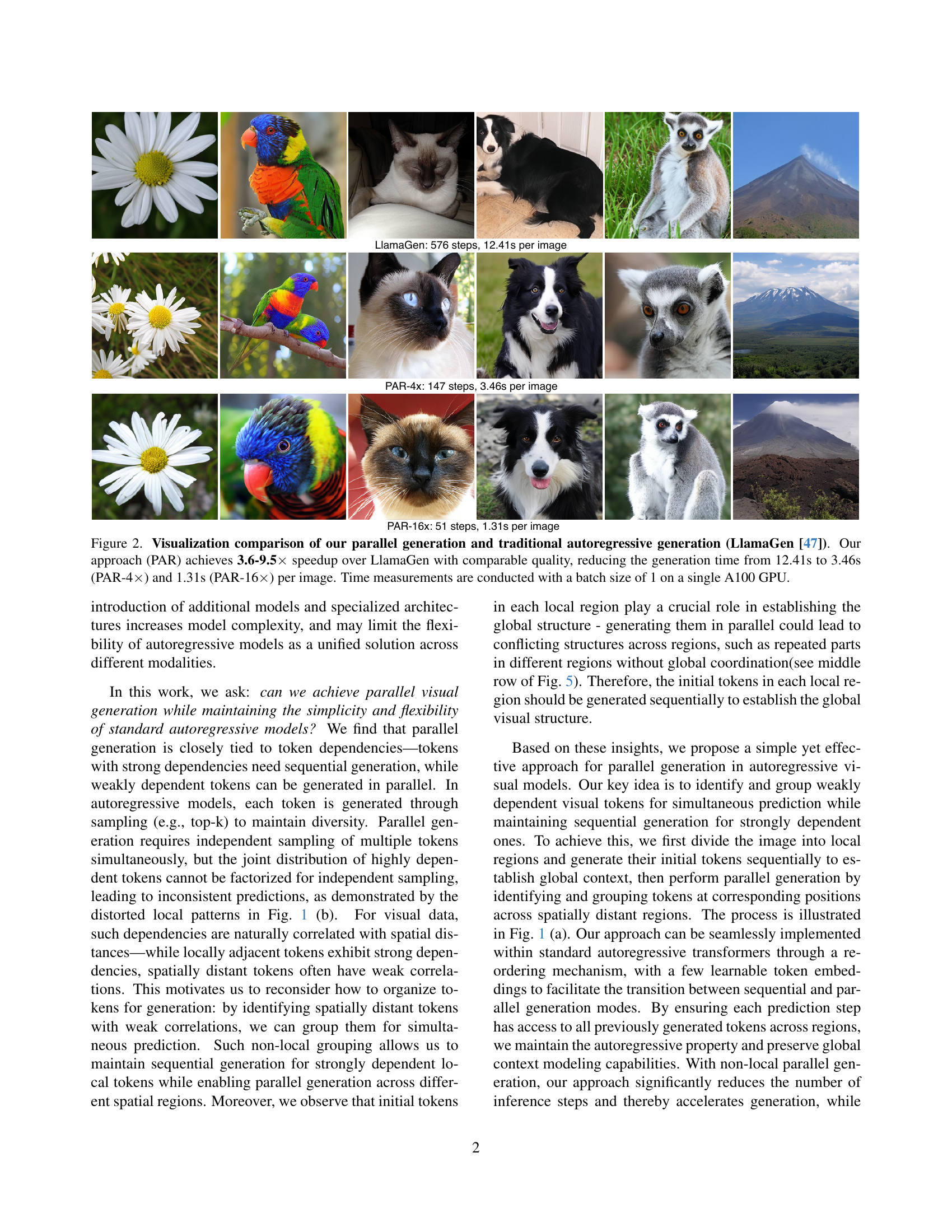
🔼 Figure 2 presents a visual comparison of image generation results using the proposed parallelized autoregressive method (PAR) and a traditional autoregressive approach (LlamaGen). The figure shows generated images side-by-side, highlighting the comparable visual quality achieved by both methods. Quantitatively, PAR demonstrates significant speed improvements, achieving a 3.6 to 9.5 times speedup over LlamaGen. Specifically, generation time is reduced from 12.41 seconds per image for LlamaGen to 3.46 seconds (PAR-4x) and 1.31 seconds (PAR-16x) for the proposed method. All timings were measured using a batch size of 1 on a single A100 GPU. The improvements showcase the efficiency gains from PAR’s parallelization strategy without compromising image quality.
read the caption
Figure 2: Visualization comparison of our parallel generation and traditional autoregressive generation (LlamaGen [47]). Our approach (PAR) achieves 3.6-9.5×\times× speedup over LlamaGen with comparable quality, reducing the generation time from 12.41s to 3.46s (PAR-4×\times×) and 1.31s (PAR-16×\times×) per image. Time measurements are conducted with a batch size of 1 on a single A100 GPU.

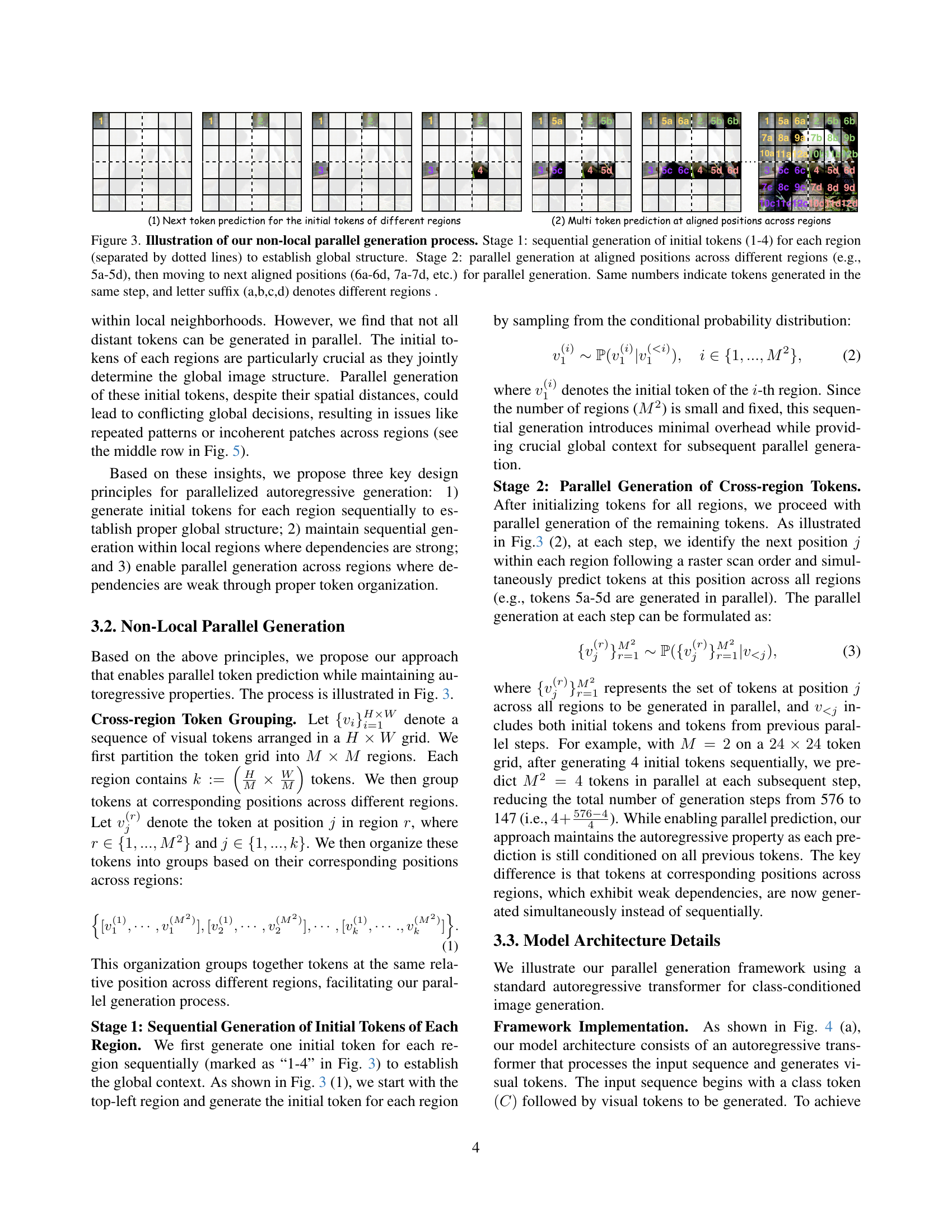
🔼 This figure illustrates the two-stage process of the proposed non-local parallel generation method. Stage 1 shows the sequential generation of initial tokens (1-4) in each region, which establishes the global image structure. Stage 2 demonstrates parallel generation of tokens at aligned positions across different regions. For instance, tokens 5a-5d are generated concurrently, followed by tokens 6a-6d, 7a-7d and so forth. The same numbers denote tokens generated in the same step, while the letter suffixes (a, b, c, d) indicate different regions. This approach aims to balance the speed benefits of parallelism with the accuracy of autoregressive modeling.
read the caption
Figure 3: Illustration of our non-local parallel generation process. Stage 1: sequential generation of initial tokens (1-4) for each region (separated by dotted lines) to establish global structure. Stage 2: parallel generation at aligned positions across different regions (e.g., 5a-5d), then moving to next aligned positions (6a-6d, 7a-7d, etc.) for parallel generation. Same numbers indicate tokens generated in the same step, and letter suffix (a,b,c,d) denotes different regions .

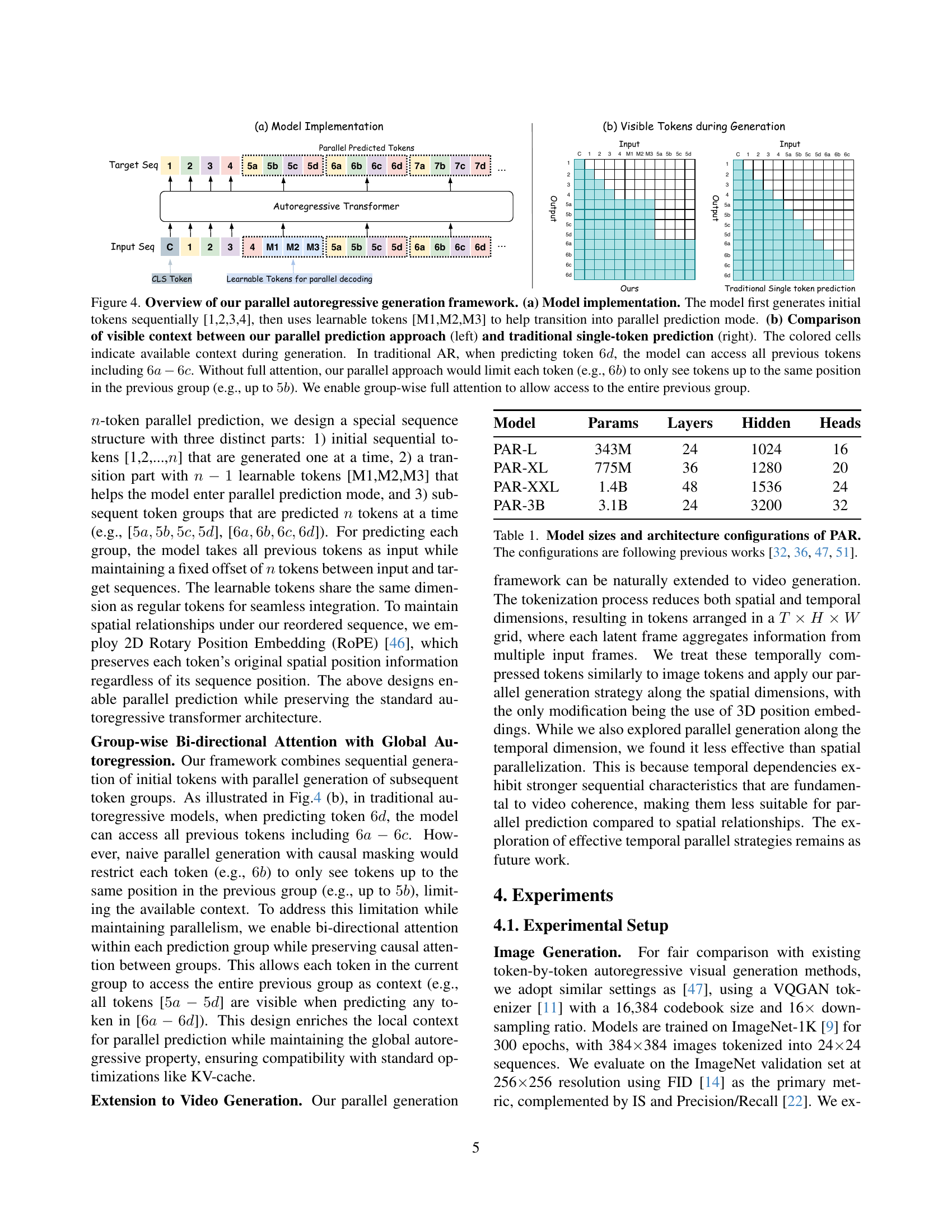
🔼 Figure 4 illustrates the proposed parallel autoregressive generation framework. Panel (a) shows the model’s architecture. It first generates initial tokens sequentially (1, 2, 3, 4), then uses special ’learnable tokens’ (M1, M2, M3) to smoothly transition to a parallel prediction mode for the remaining tokens. Panel (b) compares the visible context during generation between the proposed method and the standard autoregressive method. The standard approach allows access to all previous tokens when predicting a new one (e.g., when predicting 6d, it can see 6a-6c). In contrast, a naive parallel method would limit a token’s visibility to tokens at the same position in the previous group (e.g., when predicting 6b, only 5b would be visible). The proposed method uses group-wise full attention to allow each parallel token to see the entire previous group, overcoming this limitation.
read the caption
Figure 4: Overview of our parallel autoregressive generation framework. (a) Model implementation. The model first generates initial tokens sequentially [1,2,3,4], then uses learnable tokens [M1,M2,M3] to help transition into parallel prediction mode. (b) Comparison of visible context between our parallel prediction approach (left) and traditional single-token prediction (right). The colored cells indicate available context during generation. In traditional AR, when predicting token 6d6𝑑6d6 italic_d, the model can access all previous tokens including 6a−6c6𝑎6𝑐6a-6c6 italic_a - 6 italic_c. Without full attention, our parallel approach would limit each token (e.g., 6b6𝑏6b6 italic_b) to only see tokens up to the same position in the previous group (e.g., up to 5b5𝑏5b5 italic_b). We enable group-wise full attention to allow access to the entire previous group.

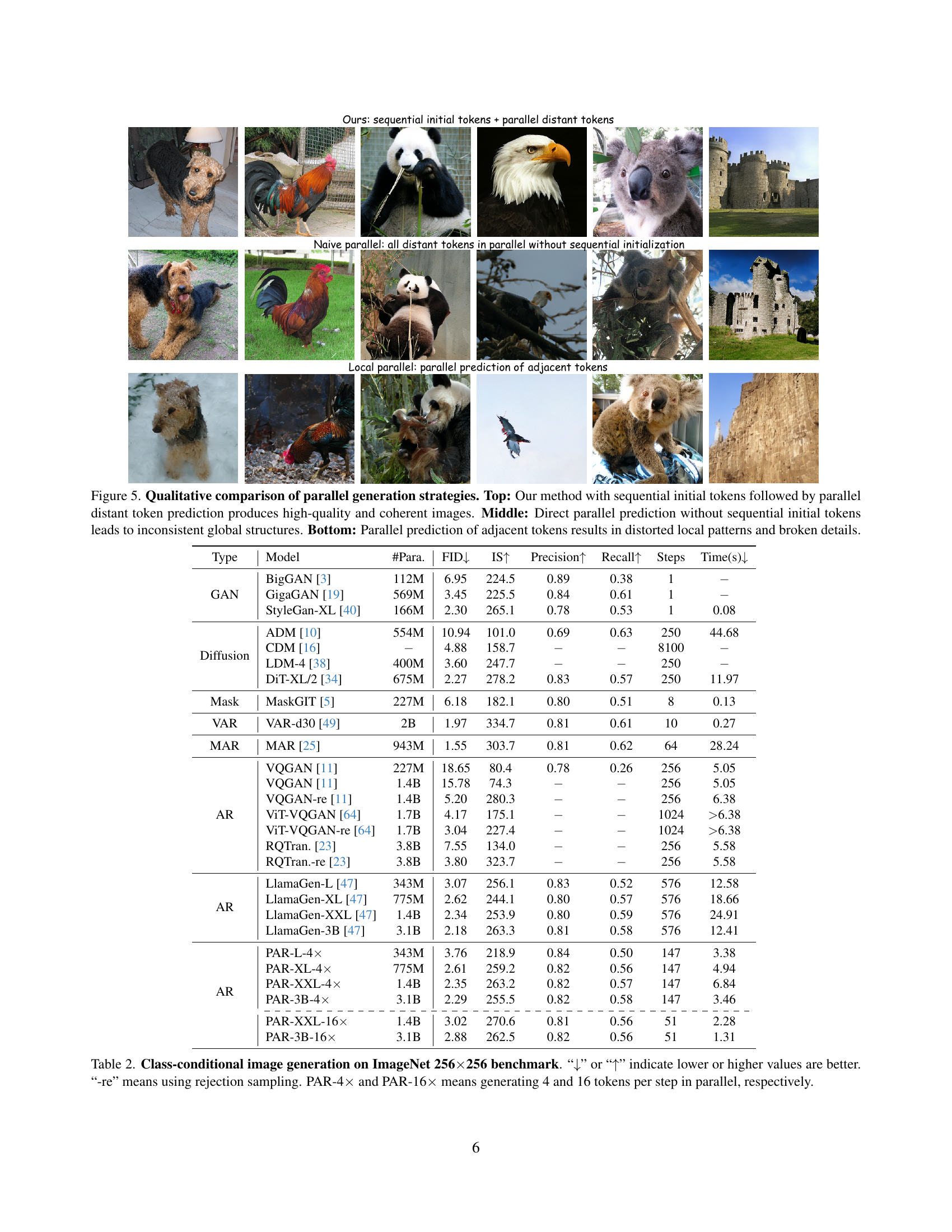
🔼 This figure compares three different parallel image generation strategies. The top row shows the results of the proposed method, which generates initial tokens sequentially to establish a global structure, followed by parallel generation of distant, weakly dependent tokens. This approach produces high-quality and coherent images. The middle row demonstrates the results of direct parallel prediction without sequential initialization. This leads to inconsistent global structures, such as repeated patterns or incoherent patches. The bottom row illustrates the outcome of parallel prediction of adjacent tokens. Due to the strong dependencies between adjacent tokens, independent sampling leads to distorted local patterns and broken details, resulting in poor image quality.
read the caption
Figure 5: Qualitative comparison of parallel generation strategies. Top: Our method with sequential initial tokens followed by parallel distant token prediction produces high-quality and coherent images. Middle: Direct parallel prediction without sequential initial tokens leads to inconsistent global structures. Bottom: Parallel prediction of adjacent tokens results in distorted local patterns and broken details.

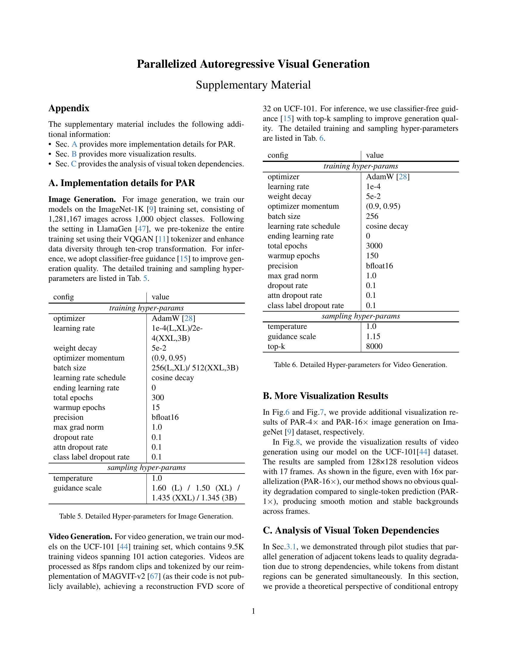
🔼 This figure displays a collection of images generated using the PAR-4x model. The images showcase the model’s ability to generate diverse and visually appealing images across a range of ImageNet object categories. Each image represents a different category, highlighting the model’s versatility and capability for high-quality image synthesis.
read the caption
Figure 6: Additional image generation results of PAR-4×\times× across different ImageNet [9] categories.

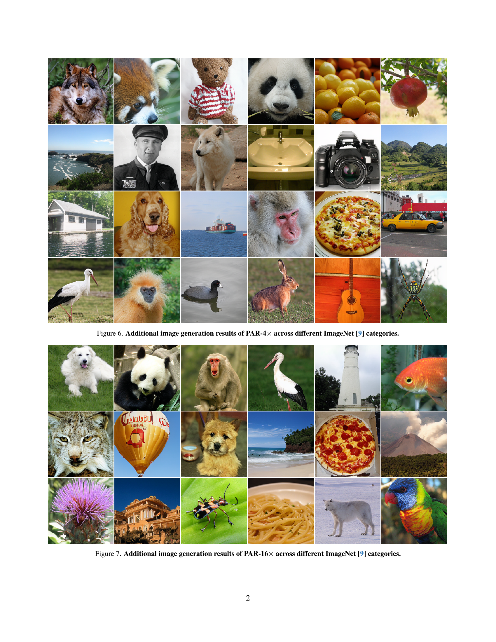
🔼 This figure displays a grid of images generated using the PAR-16x model, demonstrating its ability to produce high-quality images across various categories from the ImageNet dataset. Each image showcases a different object or scene, highlighting the model’s versatility in generating diverse visual content. The large-scale parallelization of the PAR-16x model is exemplified in the speed and efficiency with which these images were generated.
read the caption
Figure 7: Additional image generation results of PAR-16×\times× across different ImageNet [9] categories.

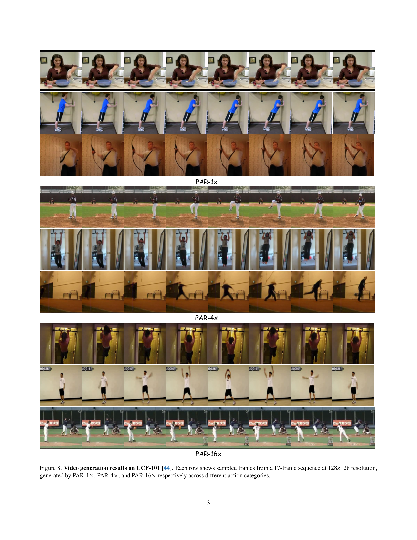
🔼 Figure 8 showcases video generation results from the UCF-101 dataset [44]. Each row displays sample frames extracted from a 17-frame video sequence. The videos have a resolution of 128x128 pixels. Three different models, PAR-1x, PAR-4x, and PAR-16x, are shown, representing varying degrees of parallelization in the video generation process. The results demonstrate the capability of each model to generate videos from different action categories within the UCF-101 dataset.
read the caption
Figure 8: Video generation results on UCF-101 [44]. Each row shows sampled frames from a 17-frame sequence at 128×128 resolution, generated by PAR-1×\times×, PAR-4×\times×, and PAR-16×\times× respectively across different action categories.

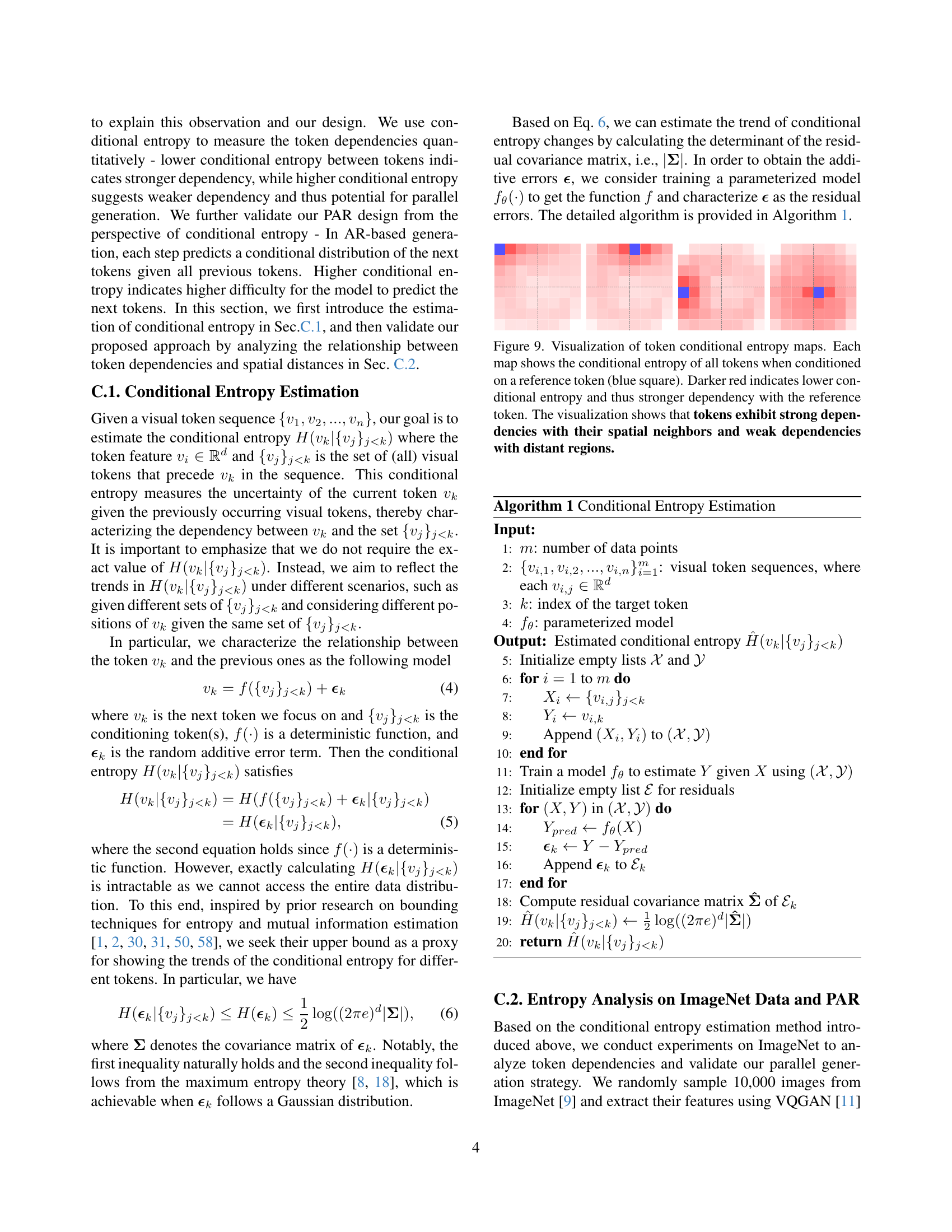
🔼 This figure visualizes the conditional entropy between tokens in an image. Each image shows the conditional entropy of all tokens given a single reference token (shown as a blue square). The color intensity represents the strength of the dependency; darker red indicates a lower conditional entropy, representing a stronger dependency with the reference token. The visualization demonstrates that tokens have strong dependencies with their spatial neighbors, while dependencies weaken significantly with distance.
read the caption
Figure 9: Visualization of token conditional entropy maps. Each map shows the conditional entropy of all tokens when conditioned on a reference token (blue square). Darker red indicates lower conditional entropy and thus stronger dependency with the reference token. The visualization shows that tokens exhibit strong dependencies with their spatial neighbors and weak dependencies with distant regions.

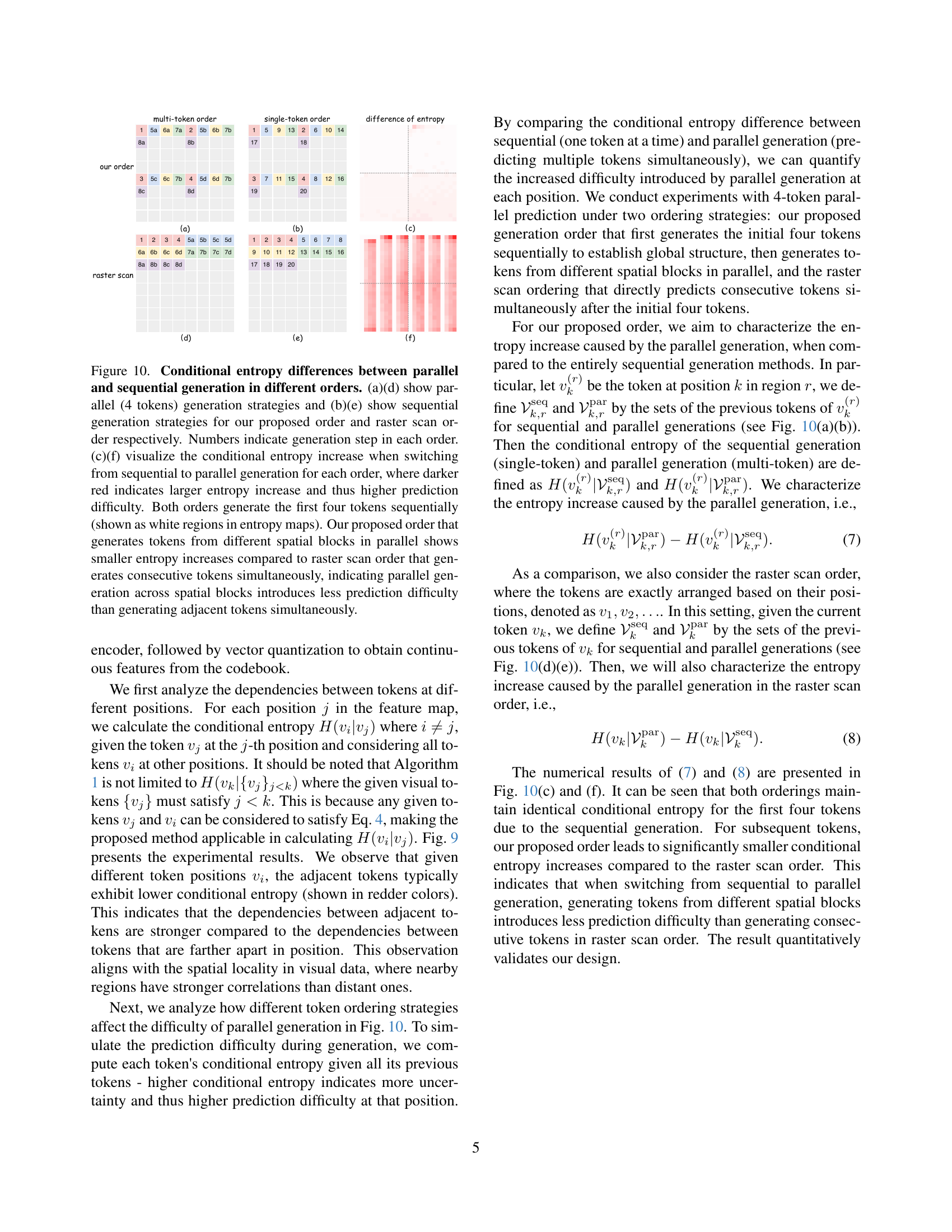
🔼 Figure 10 compares the conditional entropy increase when switching from sequential to parallel generation for two different token ordering strategies: the authors’ proposed strategy and a raster scan. The proposed strategy generates initial tokens sequentially, then groups spatially distant tokens for parallel generation, while the raster scan generates adjacent tokens in parallel. The figure visually demonstrates that the proposed strategy yields a smaller entropy increase, indicating less prediction difficulty when parallelizing across spatial blocks compared to parallelizing adjacent tokens.
read the caption
Figure 10: Conditional entropy differences between parallel and sequential generation in different orders. (a)(d) show parallel (4 tokens) generation strategies and (b)(e) show sequential generation strategies for our proposed order and raster scan order respectively. Numbers indicate generation step in each order. (c)(f) visualize the conditional entropy increase when switching from sequential to parallel generation for each order, where darker red indicates larger entropy increase and thus higher prediction difficulty. Both orders generate the first four tokens sequentially (shown as white regions in entropy maps). Our proposed order that generates tokens from different spatial blocks in parallel shows smaller entropy increases compared to raster scan order that generates consecutive tokens simultaneously, indicating parallel generation across spatial blocks introduces less prediction difficulty than generating adjacent tokens simultaneously.
More on tables
| Type | Model | #Para. | FID↓ | IS↑ | Precision↑ | Recall↑ | Steps | Time(s)↓ |
|---|---|---|---|---|---|---|---|---|
| GAN | BigGAN [3] | 112M | 6.95 | 224.5 | 0.89 | 0.38 | 1 | - |
| GigaGAN [19] | 569M | 3.45 | 225.5 | 0.84 | 0.61 | 1 | - | |
| StyleGan-XL [40] | 166M | 2.30 | 265.1 | 0.78 | 0.53 | 1 | 0.08 | |
| Diffusion | ADM [10] | 554M | 10.94 | 101.0 | 0.69 | 0.63 | 250 | 44.68 |
| CDM [16] | - | 4.88 | 158.7 | - | - | 8100 | - | |
| LDM-4 [38] | 400M | 3.60 | 247.7 | - | - | 250 | - | |
| DiT-XL/2 [34] | 675M | 2.27 | 278.2 | 0.83 | 0.57 | 250 | 11.97 | |
| Mask | MaskGIT [5] | 227M | 6.18 | 182.1 | 0.80 | 0.51 | 8 | 0.13 |
| VAR | VAR-d30 [49] | 2B | 1.97 | 334.7 | 0.81 | 0.61 | 10 | 0.27 |
| MAR | MAR [25] | 943M | 1.55 | 303.7 | 0.81 | 0.62 | 64 | 28.24 |
| AR | VQGAN [11] | 227M | 18.65 | 80.4 | 0.78 | 0.26 | 256 | 5.05 |
| VQGAN [11] | 1.4B | 15.78 | 74.3 | - | - | 256 | 5.05 | |
| VQGAN-re [11] | 1.4B | 5.20 | 280.3 | - | - | 256 | 6.38 | |
| ViT-VQGAN [64] | 1.7B | 4.17 | 175.1 | - | - | 1024 | >6.38 | |
| ViT-VQGAN-re [64] | 1.7B | 3.04 | 227.4 | - | - | 1024 | >6.38 | |
| RQTran. [23] | 3.8B | 7.55 | 134.0 | - | - | 256 | 5.58 | |
| RQTran.-re [23] | 3.8B | 3.80 | 323.7 | - | - | 256 | 5.58 | |
| LlamaGen-L [47] | 343M | 3.07 | 256.1 | 0.83 | 0.52 | 576 | 12.58 | |
| LlamaGen-XL [47] | 775M | 2.62 | 244.1 | 0.80 | 0.57 | 576 | 18.66 | |
| LlamaGen-XXL [47] | 1.4B | 2.34 | 253.9 | 0.80 | 0.59 | 576 | 24.91 | |
| LlamaGen-3B [47] | 3.1B | 2.18 | 263.3 | 0.81 | 0.58 | 576 | 12.41 | |
| AR | PAR-L-4× | 343M | 3.76 | 218.9 | 0.84 | 0.50 | 147 | 3.38 |
| PAR-XL-4× | 775M | 2.61 | 259.2 | 0.82 | 0.56 | 147 | 4.94 | |
| PAR-XXL-4× | 1.4B | 2.35 | 263.2 | 0.82 | 0.57 | 147 | 6.84 | |
| PAR-3B-4× | 3.1B | 2.29 | 255.5 | 0.82 | 0.58 | 147 | 3.46 | |
| PAR-XXL-16× | 1.4B | 3.02 | 270.6 | 0.81 | 0.56 | 51 | 2.28 | |
| PAR-3B-16× | 3.1B | 2.88 | 262.5 | 0.82 | 0.56 | 51 | 1.31 |
🔼 This table presents a quantitative comparison of various class-conditional image generation models on the ImageNet dataset at a resolution of 256x256 pixels. The models are evaluated across multiple metrics: Fréchet Inception Distance (FID), Inception Score (IS), Precision, Recall, the number of generation steps required, and the generation time. Lower FID scores indicate better image quality, while higher IS scores reflect better image diversity and quality. Precision and Recall measure how well the generated images match the target classes. The number of steps and generation time provide a measure of the computational efficiency of each model. The table includes both autoregressive (AR) and non-autoregressive models, showing the performance of the proposed method (PAR) in comparison. The ‘-re’ suffix denotes models that use rejection sampling, while PAR-4x and PAR-16x represent variations of the proposed parallel generation approach that process 4 and 16 tokens per step, respectively.
read the caption
Table 2: Class-conditional image generation on ImageNet 256×\times×256 benchmark. “↓↓\downarrow↓” or “↑↑\uparrow↑” indicate lower or higher values are better. “-re” means using rejection sampling. PAR-4×\times× and PAR-16×\times× means generating 4 and 16 tokens per step in parallel, respectively.
| FID↓ | IS↑ | steps↓ | |
|---|---|---|---|
| w/o | 3.67 | 221.36 | 144 |
| w | 2.61 | 259.17 | 147 |
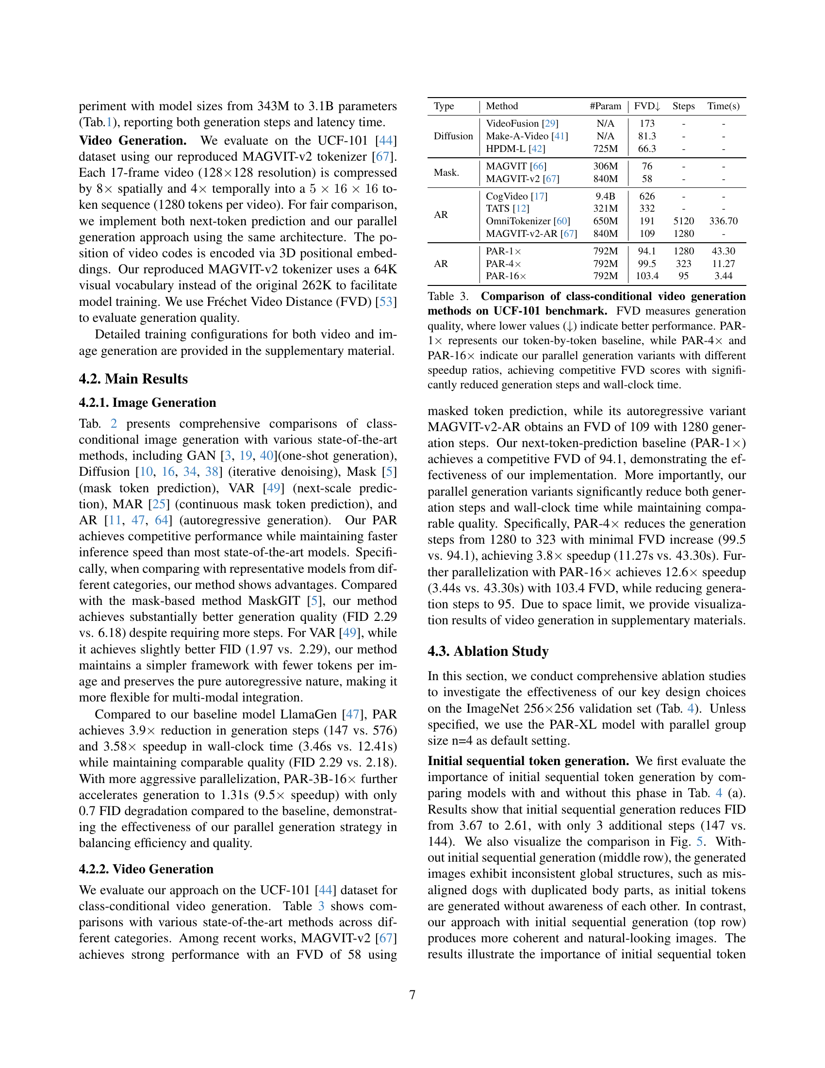
🔼 This table compares the performance of various class-conditional video generation methods on the UCF-101 benchmark dataset. The Fréchet Video Distance (FVD) metric is used to evaluate the quality of the generated videos, with lower FVD scores indicating better video generation quality. The table includes results for several state-of-the-art methods as well as the proposed method (PAR) with three different parallelization levels: PAR-1x (token-by-token baseline), PAR-4x (parallel generation with 4-fold speedup), and PAR-16x (parallel generation with 16-fold speedup). The table shows the number of parameters, FVD scores, number of steps, and generation time for each method. The results demonstrate that the proposed PAR method, particularly with higher parallelization levels, achieves competitive video generation quality with significantly reduced generation time and steps.
read the caption
Table 3: Comparison of class-conditional video generation methods on UCF-101 benchmark. FVD measures generation quality, where lower values (↓↓\downarrow↓) indicate better performance. PAR-1×\times× represents our token-by-token baseline, while PAR-4×\times× and PAR-16×\times× indicate our parallel generation variants with different speedup ratios, achieving competitive FVD scores with significantly reduced generation steps and wall-clock time.
| n | FID↓ | IS↑ | steps↓ |
|---|---|---|---|
| 1 | 2.34 | 253.90 | 576 |
| 4 | 2.35 | 263.24 | 147 |
| 16 | 3.02 | 270.57 | 51 |
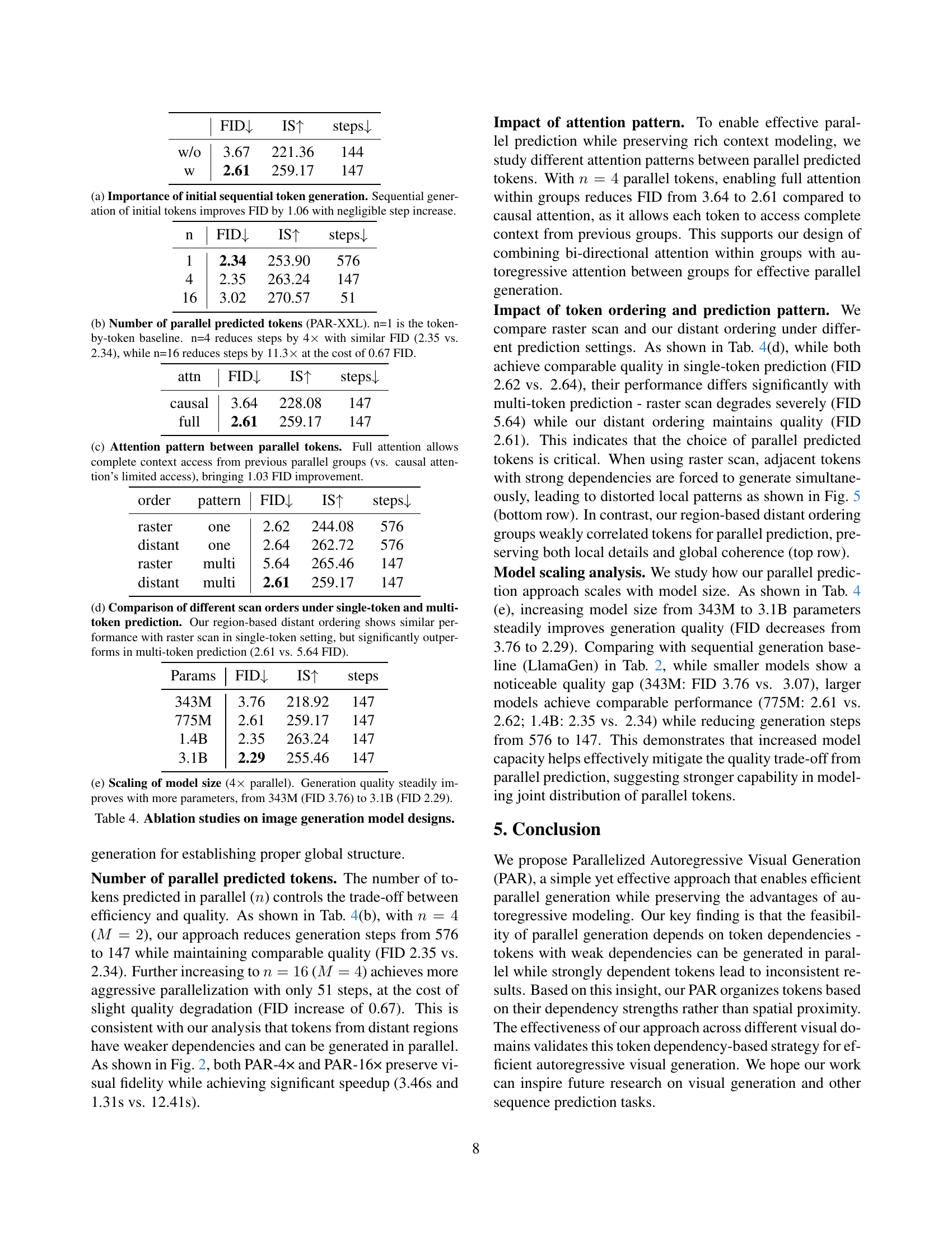
🔼 This table presents an ablation study analyzing the impact of sequentially generating initial tokens before parallel generation in the proposed parallel autoregressive visual generation method. The study compares the Fréchet Inception Distance (FID), Inception Score (IS), and number of steps required for generation with and without the initial sequential generation phase. The results demonstrate a significant improvement in FID (a lower FID indicates better image quality) when initial tokens are generated sequentially, highlighting the importance of establishing a strong global structure before parallel processing.
read the caption
(a) Importance of initial sequential token generation. Sequential generation of initial tokens improves FID by 1.06 with negligible step increase.
| attn | FID ↓ | IS ↑ | steps ↓ |
|---|---|---|---|
| causal | 3.64 | 228.08 | 147 |
| full | 2.61 | 259.17 | 147 |
🔼 This table presents ablation study results on the effect of varying the number of parallel predicted tokens (n) in the PAR-XXL model. It compares three settings: n=1 (sequential, token-by-token generation serving as the baseline), n=4 (parallel generation of 4 tokens per step), and n=16 (parallel generation of 16 tokens per step). The results show the impact on FID (Fréchet Inception Distance, a measure of image quality), IS (Inception Score), and the number of generation steps required. The key takeaway is that increasing the degree of parallelism (from n=4 to n=16) significantly reduces the number of steps needed for image generation but comes at a small cost in terms of FID (a slight decrease in image quality).
read the caption
(b) Number of parallel predicted tokens (PAR-XXL). n=1 is the token-by-token baseline. n=4 reduces steps by 4×\times× with similar FID (2.35 vs. 2.34), while n=16 reduces steps by 11.3×\times× at the cost of 0.67 FID.
| order | pattern | FID↓ | IS↑ | steps↓ |
|---|---|---|---|---|
| raster | one | 2.62 | 244.08 | 576 |
| distant | one | 2.64 | 262.72 | 576 |
| raster | multi | 5.64 | 265.46 | 147 |
| distant | multi | 2.61 | 259.17 | 147 |
🔼 This table investigates the impact of different attention mechanisms on the model’s performance when predicting multiple tokens in parallel. Specifically, it compares using ‘full attention’ (where each parallel token has access to the full context from previous groups of parallel tokens) versus ‘causal attention’ (where each parallel token only has access to the context from previous tokens in its own group or earlier groups). The results show that full attention leads to a 1.03 point improvement in FID score, indicating that providing complete contextual information is crucial for maintaining accuracy during parallel generation.
read the caption
(c) Attention pattern between parallel tokens. Full attention allows complete context access from previous parallel groups (vs. causal attention’s limited access), bringing 1.03 FID improvement.
| Params | FID ↓ | IS ↑ | steps |
|---|---|---|---|
| 343M | 3.76 | 218.92 | 147 |
| 775M | 2.61 | 259.17 | 147 |
| 1.4B | 2.35 | 263.24 | 147 |
| 3.1B | 2.29 | 255.46 | 147 |
🔼 This table compares the performance of different token ordering strategies for both single-token and multi-token prediction in autoregressive visual generation. Two scanning methods are compared: a raster scan (processing tokens sequentially from left-to-right, top-to-bottom) and a region-based distant ordering (the approach proposed by the authors, which prioritizes non-adjacent tokens in parallel prediction to leverage weak dependencies). The results show that both strategies perform comparably for single-token prediction. However, in multi-token prediction, the proposed region-based distant ordering substantially outperforms the raster scan, demonstrating its effectiveness in handling token dependencies during parallel generation. This is measured by FID (Fréchet Inception Distance) score, where a lower score indicates better image quality. The region-based distant ordering achieves a FID of 2.61, while the raster scan results in a significantly worse FID score of 5.64.
read the caption
(d) Comparison of different scan orders under single-token and multi-token prediction. Our region-based distant ordering shows similar performance with raster scan in single-token setting, but significantly outperforms in multi-token prediction (2.61 vs. 5.64 FID).
| config | value |
|---|---|
| training hyper-params | |
| — | — |
| optimizer | AdamW [28] |
| learning rate | 1e-4(L,XL)/2e-4(XXL,3B) |
| weight decay | 5e-2 |
| optimizer momentum | (0.9, 0.95) |
| batch size | 256(L,XL)/ 512(XXL,3B) |
| learning rate schedule | cosine decay |
| ending learning rate | 0 |
| total epochs | 300 |
| warmup epochs | 15 |
| precision | bfloat16 |
| max grad norm | 1.0 |
| dropout rate | 0.1 |
| attn dropout rate | 0.1 |
| class label dropout rate | 0.1 |
| sampling hyper-params | |
| — | — |
| temperature | 1.0 |
| guidance scale | 1.60 (L) / 1.50 (XL) / 1.435 (XXL) / 1.345 (3B) |
🔼 This table presents ablation study results on the impact of model size on image generation quality when using a parallel generation strategy with 4 parallel tokens per step. It shows that increasing the model size from 343 million parameters to 3.1 billion parameters leads to a consistent improvement in generation quality, as measured by the Fréchet Inception Distance (FID). The FID score decreases from 3.76 to 2.29, indicating a substantial improvement in the visual realism and quality of the generated images.
read the caption
(e) Scaling of model size (4×\times× parallel). Generation quality steadily improves with more parameters, from 343M (FID 3.76) to 3.1B (FID 2.29).
| config | value |
|---|---|
| training hyper-params | |
| — | — |
| optimizer | AdamW [28] |
| learning rate | 1e-4 |
| weight decay | 5e-2 |
| optimizer momentum | (0.9, 0.95) |
| batch size | 256 |
| learning rate schedule | cosine decay |
| ending learning rate | 0 |
| total epochs | 3000 |
| warmup epochs | 150 |
| precision | bfloat16 |
| max grad norm | 1.0 |
| dropout rate | 0.1 |
| attn dropout rate | 0.1 |
| class label dropout rate | 0.1 |
| sampling hyper-params | |
| — | — |
| temperature | 1.0 |
| guidance scale | 1.15 |
| top-k | 8000 |
🔼 This table presents the results of ablation studies conducted to analyze the impact of different design choices on the image generation model. Specifically, it investigates the importance of sequential initial token generation, the number of parallel predicted tokens, the attention mechanism used between parallel tokens, and the token ordering strategy employed. The impact of each design choice on the FID (Fréchet Inception Distance), IS (Inception Score), and the number of generation steps is quantified and compared.
read the caption
Table 4: Ablation studies on image generation model designs.
Full paper#
