↗ arXiv ↗ Hugging Face ↗ Papers with Code
TL;DR#
Autoregressive (AR) models excel in image generation but are notoriously slow due to their token-by-token process. Existing attempts to accelerate this by generating multiple tokens simultaneously fail to accurately capture the output distribution, limiting their effectiveness. This paper tackles this challenge head-on.
The proposed Distilled Decoding (DD) method leverages flow matching to create a deterministic mapping from a Gaussian distribution to the output distribution of a pre-trained AR model. A separate network is then trained to learn this mapping, enabling few-step generation. Crucially, DD’s training doesn’t need the original AR model’s data, making it practical. Experiments showcase promising results, achieving substantial speed-ups on various image AR models with acceptable fidelity loss.
Key Takeaways#
Why does it matter?#
This paper is crucial because it challenges the inherent slowness of autoregressive models, a major bottleneck in AI. By presenting a novel method to achieve one-step generation, it opens doors for efficient AR model deployment and application in real-time scenarios, impacting various fields that utilize AR, including image and text generation.
Visual Insights#

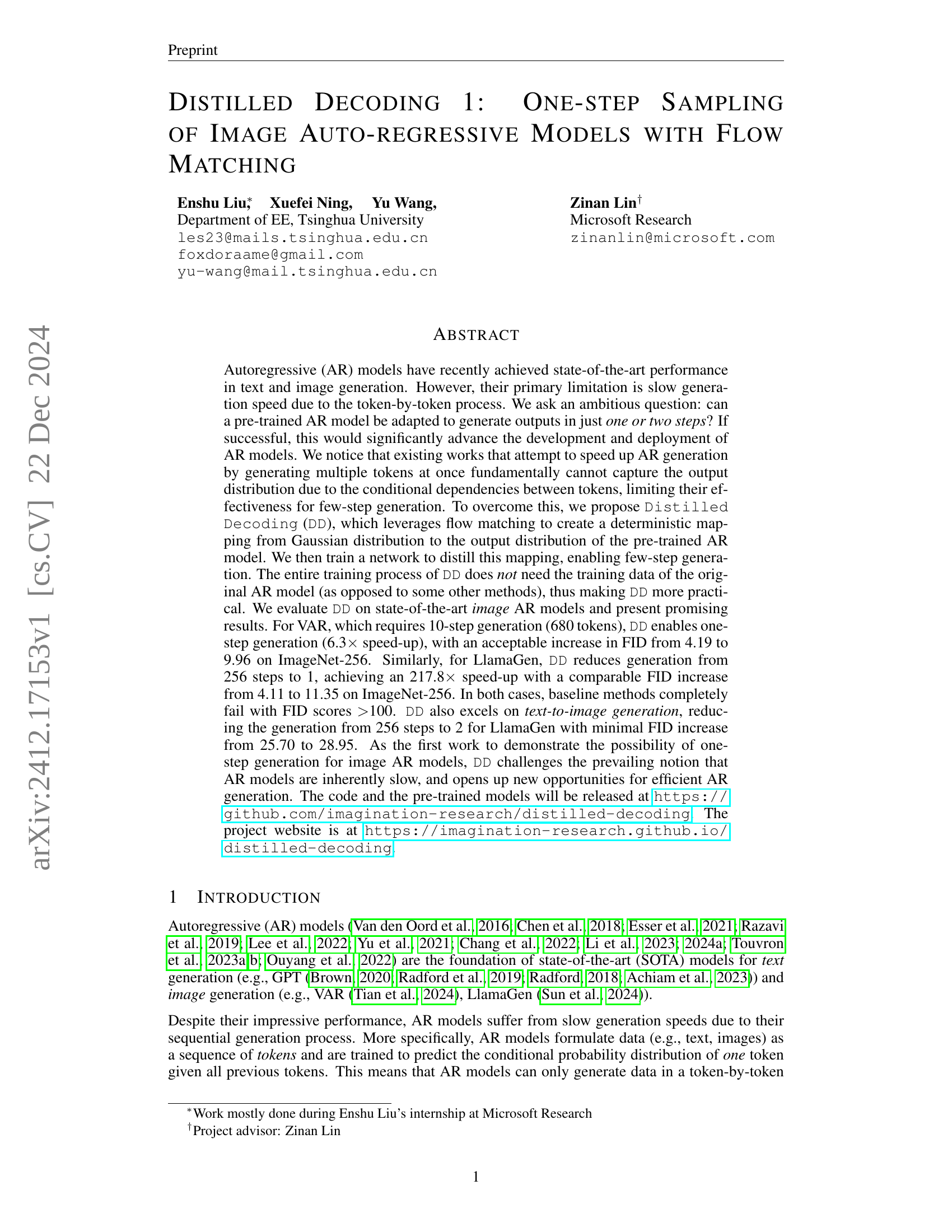
🔼 This figure presents a qualitative comparison of images generated by the proposed Distilled Decoding (DD) method and the original LlamaGen model. The comparison focuses on ImageNet 256x256 images. The results demonstrate that DD achieves a significant speedup (at least 200 times faster) compared to LlamaGen, while maintaining comparable image quality. The minimal quality loss suggests the effectiveness of DD in accelerating image generation without substantial compromise of visual fidelity. Additional examples are provided in Appendix F.
read the caption
Figure 1: Qualitative comparisons between DD and vanilla LlamaGen Sun et al. (2024) on ImageNet 256×\times×256. We show that the generated images of DD have small quality loss compared to the pre-trained AR model, while achieving ≥\geq≥200×\times× speedup. More examples are in App. F.
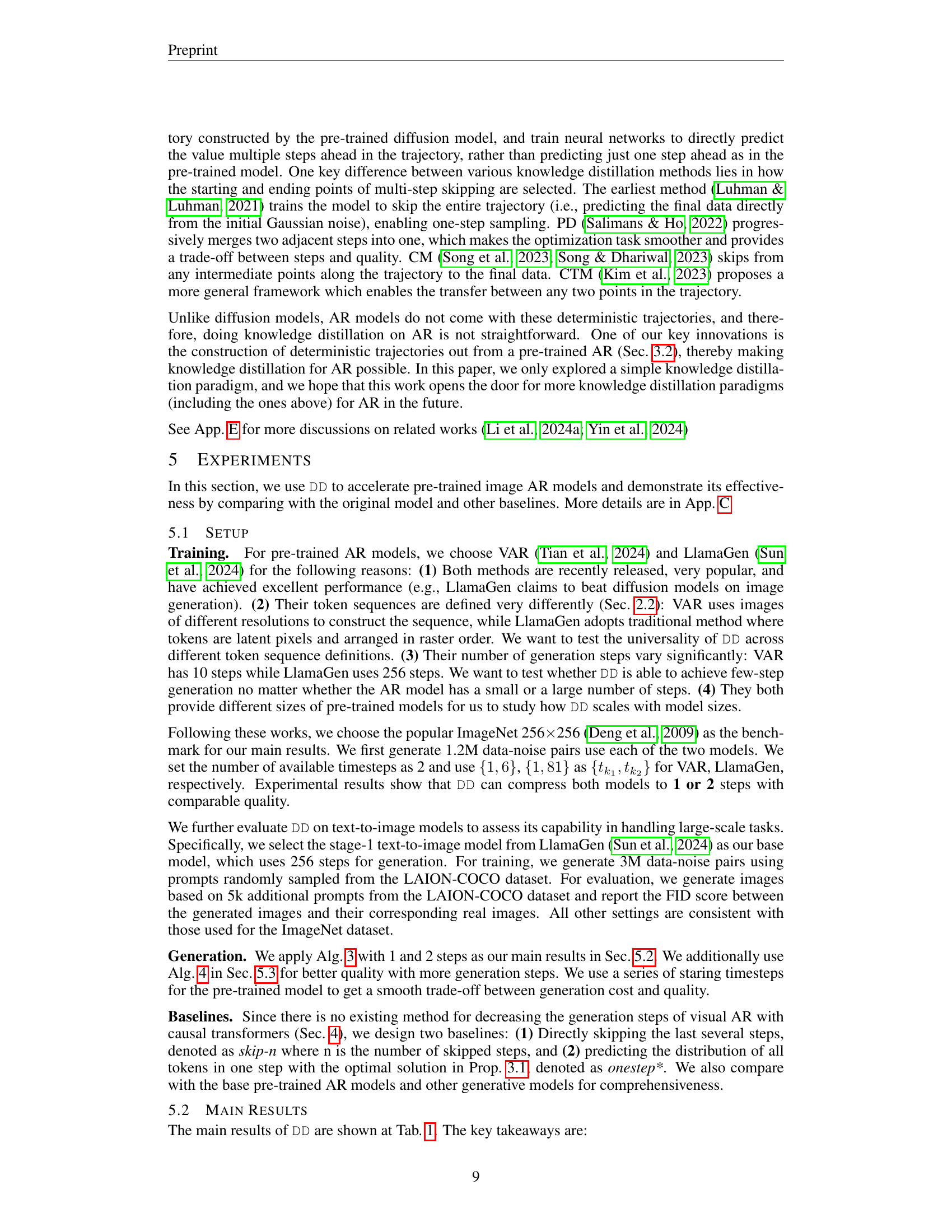
| Type | Model | FID ↓ | IS ↑ | Pre ↑ | Rec ↑ | #Para | #Step | Time |
|---|---|---|---|---|---|---|---|---|
| GAN† | StyleGan-XL (Sauer et al., 2022) | 2.30 | 265.1 | 0.78 | 0.53 | 166M | 1 | 0.3 |
| Diff.† | ADM (Dhariwal & Nichol, 2021) | 10.94 | 101.0 | 0.69 | 0.63 | 554M | 250 | 168 |
| Diff.† | LDM-4-G (Rombach et al., 2022) | 3.60 | 247.7 | - | - | 400M | 250 | - |
| Diff.† | DiT-L/2 (Peebles & Xie, 2023) | 5.02 | 167.2 | 0.75 | 0.57 | 458M | 250 | 31 |
| Diff.† | L-DiT-7B (Peebles & Xie, 2023) | 2.28 | 316.2 | 0.83 | 0.58 | 7.0B | 250 | >45 |
| Mask.† | MaskGIT (Chang et al., 2022) | 6.18 | 182.1 | 0.80 | 0.51 | 227M | 8 | 0.5 |
| AR† | VQVAE-2† (Razavi et al., 2019) | 31.11 | ~45 | 0.36 | 0.57 | 13.5B | 5120 | - |
| AR† | VQGAN† (Esser et al., 2021) | 18.65 | 80.4 | 0.78 | 0.26 | 227M | 256 | 19 |
| AR | VQGAN (Esser et al., 2021) | 15.78 | 74.3 | - | - | 1.4B | 256 | 24 |
| AR | ViTVQ (Yu et al., 2021) | 4.17 | 175.1 | - | - | 1.7B | 1024 | >24 |
| AR | RQTran. (Lee et al., 2022) | 7.55 | 134.0 | - | - | 3.8B | 68 | 21 |
| AR | VAR-d16 (Tian et al., 2024) | 4.19 | 230.2 | 0.84 | 0.48 | 310M | 10 | 0.133 |
| AR | VAR-d20 (Tian et al., 2024) | 3.35 | 301.4 | 0.84 | 0.51 | 600M | 10 | - |
| AR | VAR-d24 (Tian et al., 2024) | 2.51 | 312.2 | 0.82 | 0.53 | 1.03B | 10 | - |
| AR | LlamaGen-B (Sun et al., 2024) | 5.42 | 193.5 | 0.83 | 0.44 | 111M | 256 | - |
| AR | LlamaGen-L (Sun et al., 2024) | 4.11 | 283.5 | 0.85 | 0.48 | 343M | 256 | 5.01 |
| Baseline | VAR-skip-1 | 9.52 | 178.9 | 0.68 | 0.54 | 310M | 9 | 0.113 |
| Baseline | VAR-skip-2 | 40.09 | 56.8 | 0.46 | 0.50 | 310M | 8 | 0.098 |
| Baseline | VAR-onestep* | 157.5 | - | - | - | 1 | - | - |
| Baseline | LlamaGen-skip-106 | 19.14 | 80.39 | 0.42 | 0.43 | 343M | 150 | 2.94 |
| Baseline | LlamaGen-skip-156 | 80.72 | 12.13 | 0.17 | 0.20 | 343M | 100 | 1.95 |
| Baseline | LlamaGen-onestep* | 220.2 | - | - | - | 1 | - | - |
| Ours | VAR-d16-DD | 9.94 | 193.6 | 0.80 | 0.37 | 327M | 1 | 0.021 (6.3×) |
| Ours | VAR-d16-DD | 7.82 | 197.0 | 0.80 | 0.41 | 327M | 2 | 0.036 (3.7×) |
| Ours | VAR-d20-DD | 9.55 | 197.2 | 0.78 | 0.38 | 635M | 1 | - |
| Ours | VAR-d20-DD | 7.33 | 204.5 | 0.82 | 0.40 | 635M | 2 | - |
| Ours | VAR-d24-DD | 8.92 | 202.8 | 0.78 | 0.39 | 1.09B | 1 | - |
| Ours | VAR-d24-DD | 6.95 | 222.5 | 0.83 | 0.43 | 1.09B | 2 | - |
| Ours | LlamaGen-B-DD | 15.50 | 135.4 | 0.76 | 0.26 | 98.3M | 1 | - |
| Ours | LlamaGen-B-DD | 11.17 | 154.8 | 0.80 | 0.31 | 98.3M | 2 | - |
| Ours | LlamaGen-L-DD | 11.35 | 193.6 | 0.81 | 0.30 | 326M | 1 | 0.023 (217.8×) |
| Ours | LlamaGen-L-DD | 7.58 | 237.5 | 0.84 | 0.37 | 326M | 2 | 0.043 (116.5×) |
🔼 Table 1 presents a comparison of various image generation models on the ImageNet-256 dataset, focusing on the trade-off between generation quality and speed. The table includes several state-of-the-art autoregressive (AR) models along with the proposed Distilled Decoding (DD) method and several baselines. For each model, the table shows the Fréchet Inception Distance (FID) score, which measures the quality of the generated images; the Inception Score (IS) and Precision (Prec) scores, which are other metrics for image quality; the Recall score (Rec); the number of parameters (#Para) in the model; the number of steps required to generate an image (#Step); and the wall-clock time to generate one image (Time). The results show that the DD approach is able to significantly reduce generation time while maintaining reasonable image quality compared to the baseline and pre-trained models. Results marked with † are taken directly from the cited VAR paper.
read the caption
Table 1: Generative performance on class-conditional ImageNet-256. “#Step” indicates the number of model inference to generate one image. “Time” is the wall-time of generating one image in the steady state. Results with † are taken from the VAR paper (Tian et al., 2024).
In-depth insights#
One-step AR#
The concept of “One-step AR” in the context of autoregressive (AR) models signifies a paradigm shift towards drastically accelerating image generation. Traditional AR models generate images token by token, a process inherently slow. The innovation lies in developing methods that can generate the entire image from a single input, eliminating the sequential generation bottleneck. This presents significant challenges, primarily due to the complex conditional dependencies between tokens in an image. The paper explores this challenge by proposing a novel technique, likely leveraging flow matching or a similar method to map a simple noise distribution into the target image distribution, effectively learning a shortcut to one-step generation. The success of this approach would be measured by balancing speed gains against any decline in image quality, represented by metrics like FID scores. A key aspect is that the method may avoid needing the original AR model’s training data. This is a critical step towards practical implementation because access to large training datasets for SOTA models is often limited. Ultimately, “One-step AR” represents a promising direction for making efficient AR image generation a reality.
Flow Matching#
The concept of ‘Flow Matching’ in the context of this research paper centers on creating a deterministic mapping between a simple, known distribution (like a Gaussian) and the complex, target distribution of a pre-trained autoregressive (AR) model. This is crucial because directly sampling from the AR model’s intricate distribution is computationally expensive, requiring many sequential steps. Flow matching, therefore, provides a pathway to bypass this inefficiency by training a network to mimic the transformation learned by the flow. This transformation effectively distills the model’s complex behavior, enabling the generation of samples in significantly fewer steps. The method leverages the deterministic nature of flow-based generative models. Instead of probabilistic sampling, a deterministic function maps the simple input to the complex output distribution, making it efficient to generate the entire sequence with a single forward pass. This clever approach addresses the limitations of prior methods, which attempted parallel token generation but failed due to the inherent conditional dependencies between tokens in AR models. The key innovation lies in its ability to produce a one-to-one mapping from a simple source distribution to the target distribution without losing essential characteristics of the original AR model. The resulting speed gains, demonstrated by impressive speedups, make flow matching a compelling technique for accelerating AR model inference.
DD Training#
The effectiveness of the Distilled Decoding (DD) framework hinges significantly on its training methodology. DD training cleverly sidesteps the need for the original AR model’s training data, a crucial advantage for practical applications where such data may be unavailable or proprietary. Instead, it leverages flow matching to create a deterministic mapping between a Gaussian distribution and the target AR model’s output distribution. A neural network is then trained to learn this distilled mapping, enabling efficient few-step generation. This training process is likely computationally intensive, requiring substantial resources and careful hyperparameter tuning to balance speed and accuracy. The choice of loss function(s) (e.g., combining cross-entropy and LPIPS loss) and the implementation of techniques like exponential moving average (EMA) play crucial roles in the network’s convergence and performance. The optimal training strategy would likely involve careful experimentation with different network architectures, loss weighting schemes, and optimization algorithms, likely on a high-performance computing platform. Furthermore, understanding the interplay between training data size and model performance is critical for determining the resources needed. The scalability of the DD training process across different AR models and dataset sizes needs to be carefully investigated to ensure its generalizability and practical use in diverse scenarios.
Ablation Study#
An ablation study systematically investigates the contribution of individual components within a machine learning model. In the context of this research, it likely assesses the impact of key elements on the distilled decoding model’s performance. This could include examining the influence of different training strategies, varying the number of intermediate steps used in generation, and testing the sensitivity to dataset size and the effect of using a pre-trained AR model within the generation process. The results from the ablation study would be crucial in understanding which aspects are essential for the model’s effectiveness and identifying potential areas for future improvement. The study allows researchers to justify design choices, demonstrating that the core components are critical for the model’s overall success. By isolating and analyzing individual elements, the researchers can gain a deeper understanding of the interplay between different model components and how they contribute to the ultimate goal of efficient and high-quality image generation. This approach is essential in establishing the robustness and validity of the proposed distilled decoding method.
Future Work#
The ‘Future Work’ section of this research paper on distilled decoding for autoregressive models presents exciting avenues for further exploration. A key area is eliminating the reliance on pre-trained teacher models, which would greatly enhance the practicality and applicability of the method. This could involve exploring unsupervised or self-supervised learning techniques to learn the mapping between noisy and generated tokens directly from data. Another promising direction is applying distilled decoding to large language models (LLMs), a significantly more complex task due to the scale and structure of LLMs. Successfully adapting the technique to LLMs would be a major advancement in the field. Furthermore, investigating the optimal trade-off between inference cost and model performance is crucial. The paper suggests that current models may be over-parameterized or trained inefficiently, opening up the possibility of creating even more efficient models by fine-tuning the balance between speed and quality. Finally, combining distilled decoding with other state-of-the-art techniques such as those used in diffusion models or improving upon the existing flow-matching method, could lead to even better performance and efficiency gains.
More visual insights#
More on figures

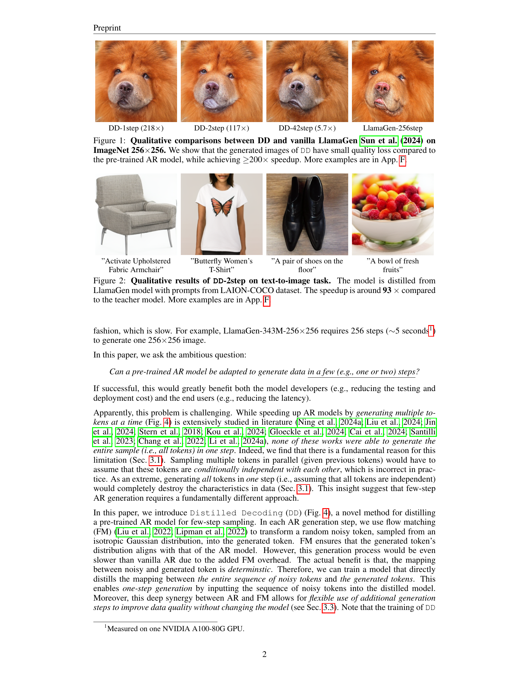
🔼 Figure 2 showcases the performance of the Distilled Decoding (DD) method’s two-step variant (DD-2step) on a text-to-image generation task. The DD-2step model is a distilled version of the LlamaGen model, meaning its parameters have been optimized to mimic LlamaGen’s behavior but with significantly improved speed. The input to the model consists of text prompts sourced from the LAION-COCO dataset. The figure displays four example image outputs generated by DD-2step, demonstrating the visual results obtained. Notably, the figure highlights the considerable speed enhancement achieved by DD-2step, achieving a 93x speedup over the original LlamaGen model. Additional examples illustrating the method’s performance can be found in Appendix F.
read the caption
Figure 2: Qualitative results of DD-2step on text-to-image task. The model is distilled from LlamaGen model with prompts from LAION-COCO dataset. The speedup is around 93 ×\times× compared to the teacher model. More examples are in App. F.

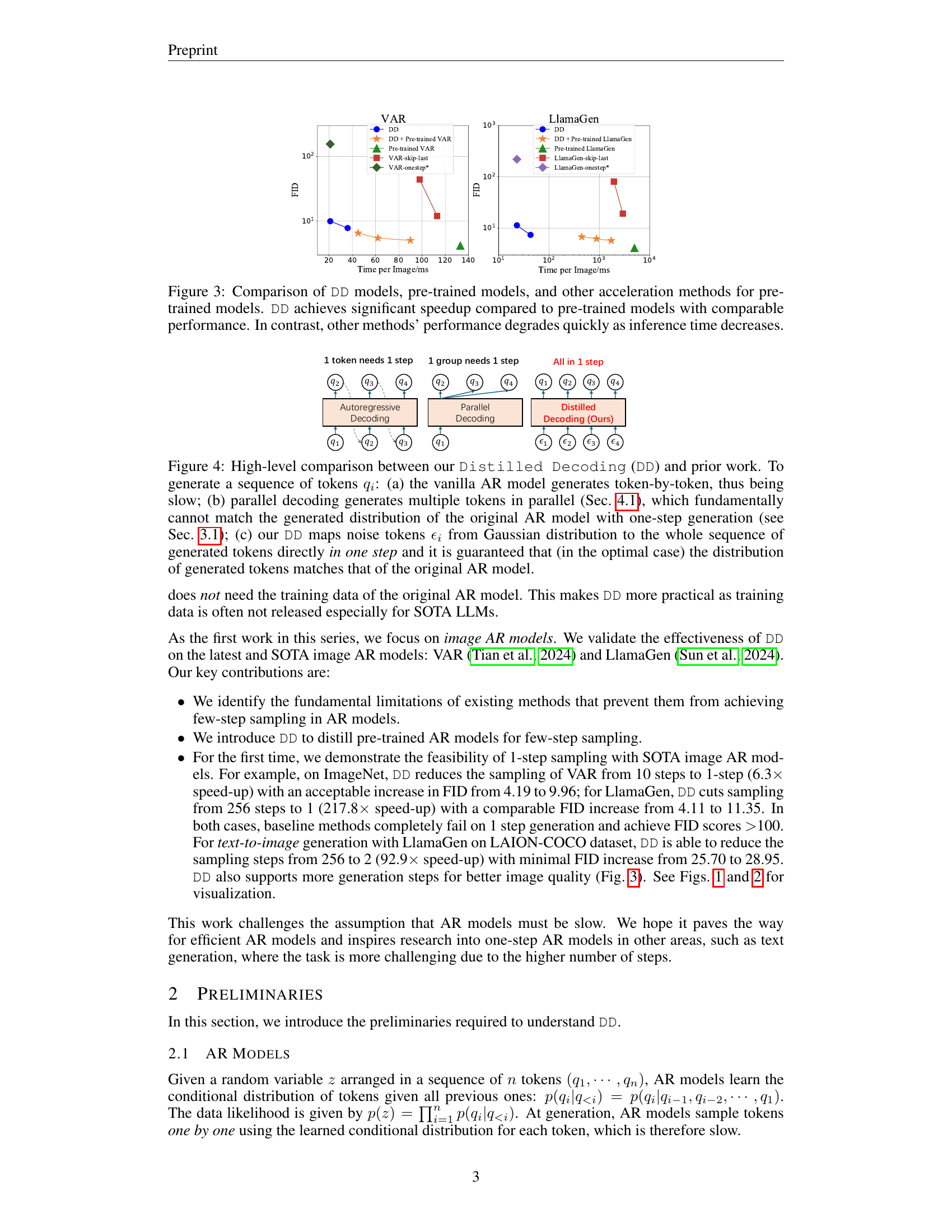
🔼 Figure 3 presents a comparison of the performance and inference speed of different methods for generating images using pretrained autoregressive models. The methods include the proposed Distilled Decoding (DD) models, the original pretrained models, and other existing acceleration techniques. The figure demonstrates that DD achieves a significant speedup over the pretrained models while maintaining comparable image quality (measured by FID). In contrast, the other acceleration techniques show a substantial decrease in image quality as their inference time is reduced.
read the caption
Figure 3: Comparison of DD models, pre-trained models, and other acceleration methods for pre-trained models. DD achieves significant speedup compared to pre-trained models with comparable performance. In contrast, other methods’ performance degrades quickly as inference time decreases.

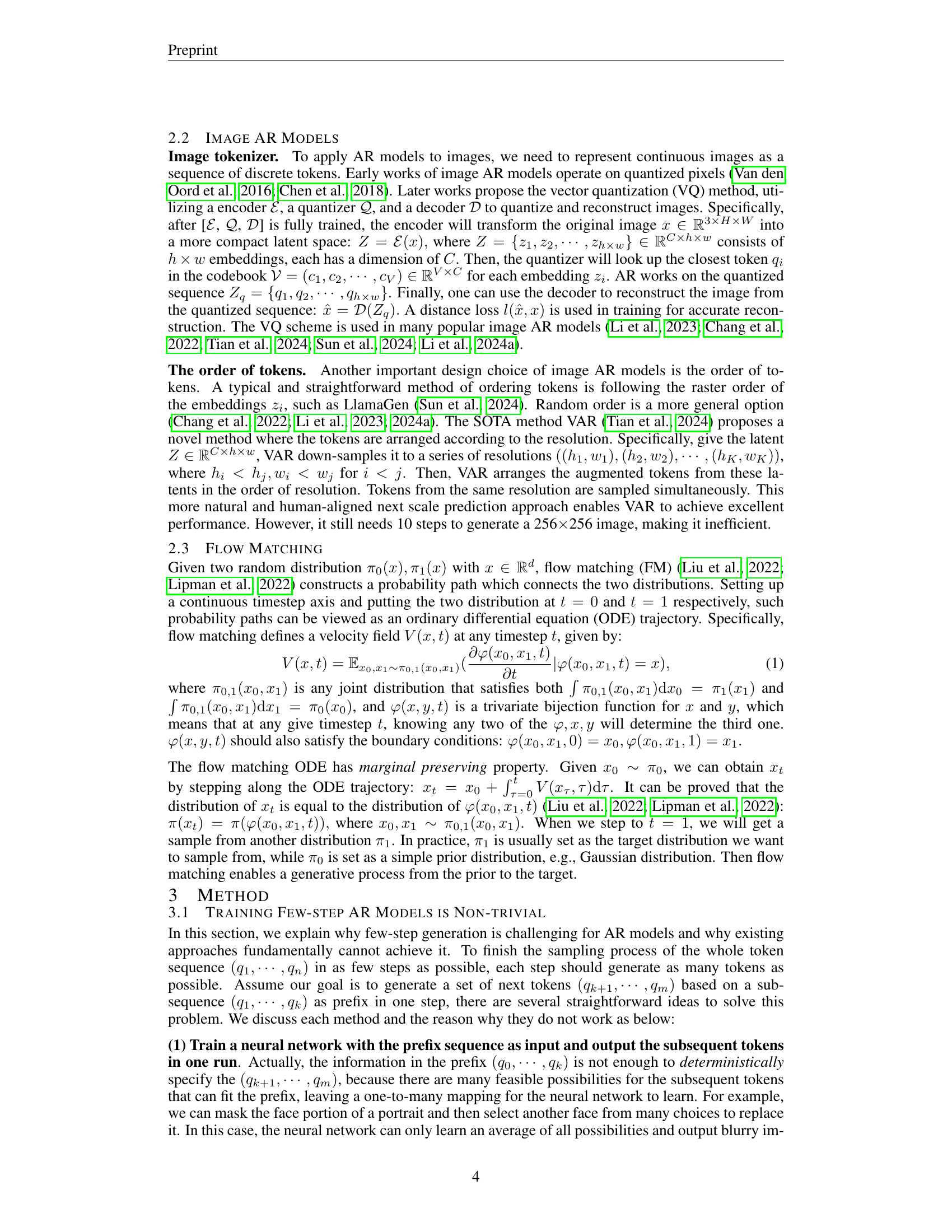
🔼 Figure 4 illustrates three approaches to generating a sequence of tokens using autoregressive (AR) models. (a) shows the standard AR approach, where tokens are generated sequentially, one at a time. This is slow but accurately reflects the token dependencies. (b) demonstrates parallel decoding, a faster approach where multiple tokens are generated simultaneously. However, this method assumes independence between tokens, leading to inaccurate output distribution, especially when generating the entire sequence in a single step. (c) presents the proposed Distilled Decoding (DD) method. DD utilizes flow matching to deterministically map noise tokens from a Gaussian distribution to the target token distribution of the pre-trained AR model. This allows the generation of the entire token sequence in one step, matching the original model’s distribution while being significantly faster.
read the caption
Figure 4: High-level comparison between our Distilled Decoding (DD) and prior work. To generate a sequence of tokens qisubscript𝑞𝑖q_{i}italic_q start_POSTSUBSCRIPT italic_i end_POSTSUBSCRIPT: (a) the vanilla AR model generates token-by-token, thus being slow; (b) parallel decoding generates multiple tokens in parallel (Sec. 4.1), which fundamentally cannot match the generated distribution of the original AR model with one-step generation (see Sec. 3.1); (c) our DD maps noise tokens ϵisubscriptitalic-ϵ𝑖\epsilon_{i}italic_ϵ start_POSTSUBSCRIPT italic_i end_POSTSUBSCRIPT from Gaussian distribution to the whole sequence of generated tokens directly in one step and it is guaranteed that (in the optimal case) the distribution of generated tokens matches that of the original AR model.

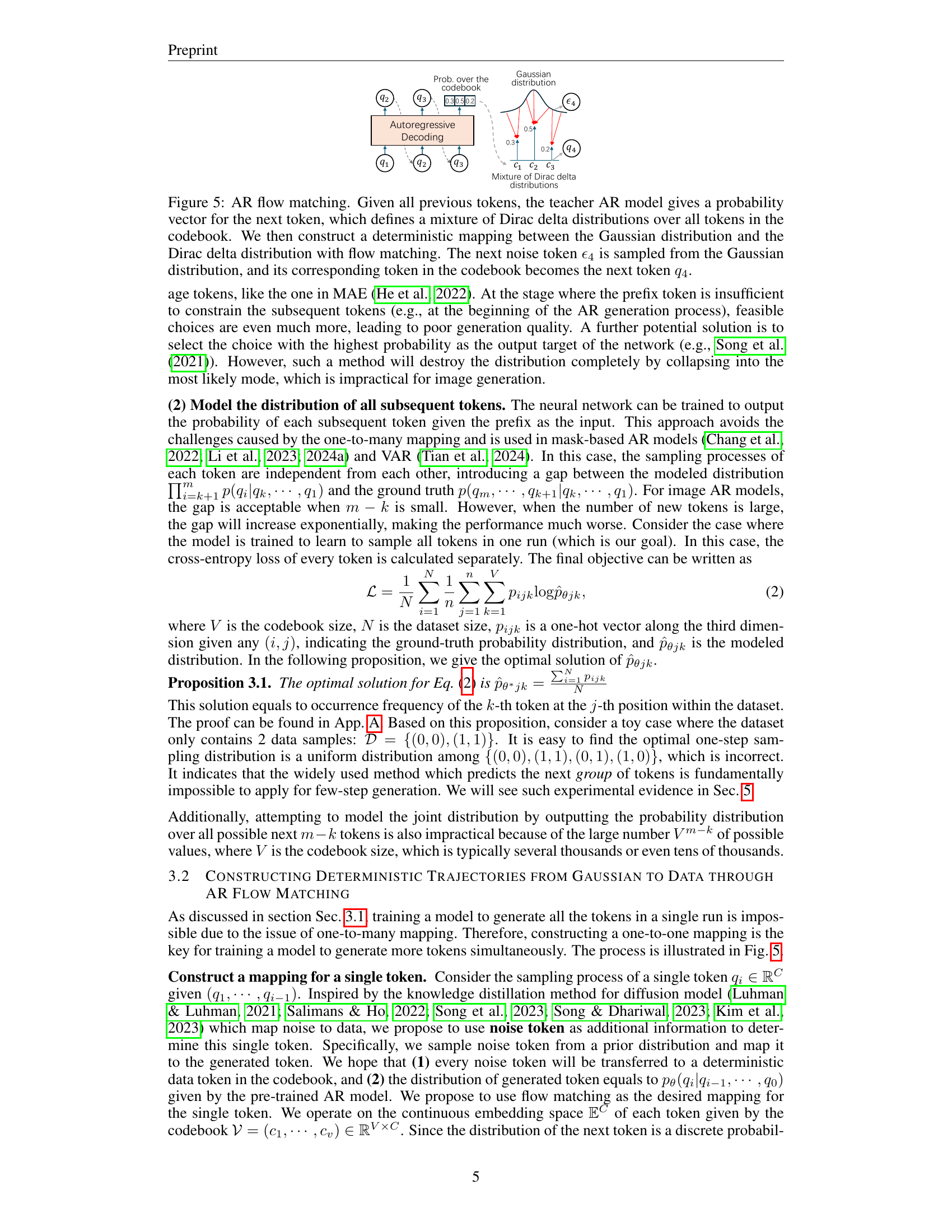
🔼 This figure illustrates the core concept of Distilled Decoding (DD). The process begins with a pre-trained autoregressive (AR) model, which, given a sequence of previous tokens (q1, q2, q3…), provides a probability distribution for the next token. This distribution is a mixture of Dirac delta functions, where each function represents a token in the codebook and its weight is its probability. DD then leverages flow matching to create a deterministic mapping between a simple Gaussian distribution and this complex, discrete probability distribution from the AR model. A sample from the Gaussian distribution (ϵ4) is transformed into a token (q4) using this deterministic mapping. This deterministic mapping is then learned by a neural network in the distillation phase. The result is that a simple noise input can be directly transformed into a valid output of the AR model, allowing for one-step or few-step sampling.
read the caption
Figure 5: AR flow matching. Given all previous tokens, the teacher AR model gives a probability vector for the next token, which defines a mixture of Dirac delta distributions over all tokens in the codebook. We then construct a deterministic mapping between the Gaussian distribution and the Dirac delta distribution with flow matching. The next noise token ϵ4subscriptitalic-ϵ4\epsilon_{4}italic_ϵ start_POSTSUBSCRIPT 4 end_POSTSUBSCRIPT is sampled from the Gaussian distribution, and its corresponding token in the codebook becomes the next token q4subscript𝑞4q_{4}italic_q start_POSTSUBSCRIPT 4 end_POSTSUBSCRIPT.

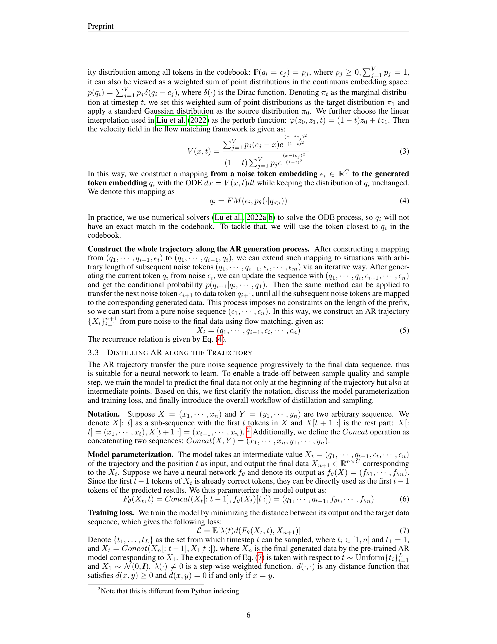
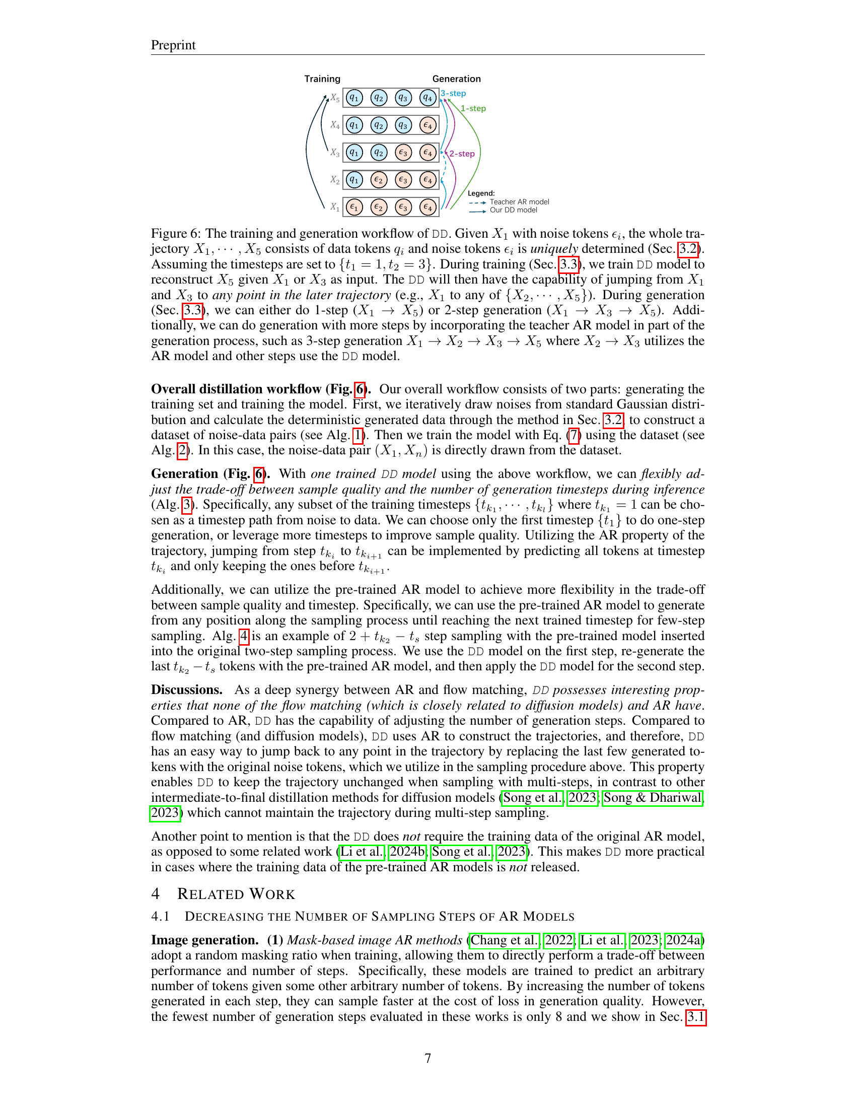
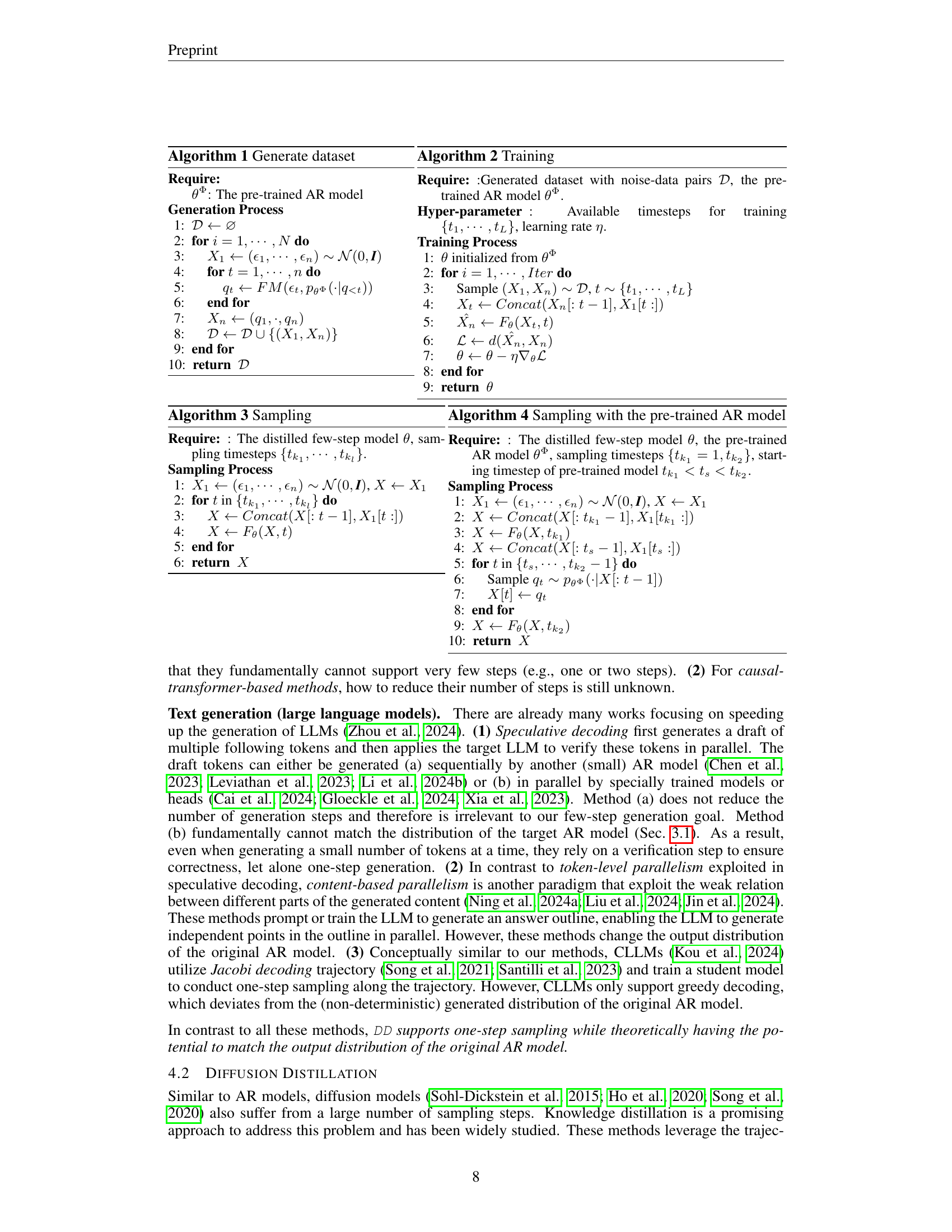
🔼 Figure 6 illustrates the training and generation workflow of the Distilled Decoding (DD) method. Starting with a sequence of noise tokens (X1), a trajectory is generated using flow matching and the pre-trained autoregressive (AR) model. This trajectory (X1, …, X5) consists of both noise and data tokens. During training, the DD model learns to reconstruct the final state of the trajectory (X5) given intermediate states (X1 or X3) as input. This enables the DD model to ‘jump’ forward in the trajectory, skipping intermediate steps. During generation, the user can choose to generate the sequence in 1 step (directly from X1 to X5), 2 steps (X1 to X3 then to X5), or more steps where parts of the trajectory leverage the pre-trained AR model for higher quality (e.g., a 3-step generation using DD for X1 to X2 and X3 to X5 and the AR model from X2 to X3).
read the caption
Figure 6: The training and generation workflow of DD. Given X1subscript𝑋1X_{1}italic_X start_POSTSUBSCRIPT 1 end_POSTSUBSCRIPT with noise tokens ϵisubscriptitalic-ϵ𝑖\epsilon_{i}italic_ϵ start_POSTSUBSCRIPT italic_i end_POSTSUBSCRIPT, the whole trajectory X1,⋯,X5subscript𝑋1⋯subscript𝑋5X_{1},\cdots,X_{5}italic_X start_POSTSUBSCRIPT 1 end_POSTSUBSCRIPT , ⋯ , italic_X start_POSTSUBSCRIPT 5 end_POSTSUBSCRIPT consists of data tokens qisubscript𝑞𝑖q_{i}italic_q start_POSTSUBSCRIPT italic_i end_POSTSUBSCRIPT and noise tokens ϵisubscriptitalic-ϵ𝑖\epsilon_{i}italic_ϵ start_POSTSUBSCRIPT italic_i end_POSTSUBSCRIPT is uniquely determined (Sec. 3.2). Assuming the timesteps are set to {t1=1,t2=3}formulae-sequencesubscript𝑡11subscript𝑡23\{t_{1}=1,t_{2}=3\}{ italic_t start_POSTSUBSCRIPT 1 end_POSTSUBSCRIPT = 1 , italic_t start_POSTSUBSCRIPT 2 end_POSTSUBSCRIPT = 3 }. During training (Sec. 3.3), we train DD model to reconstruct X5subscript𝑋5X_{5}italic_X start_POSTSUBSCRIPT 5 end_POSTSUBSCRIPT given X1subscript𝑋1X_{1}italic_X start_POSTSUBSCRIPT 1 end_POSTSUBSCRIPT or X3subscript𝑋3X_{3}italic_X start_POSTSUBSCRIPT 3 end_POSTSUBSCRIPT as input. The DD will then have the capability of jumping from X1subscript𝑋1X_{1}italic_X start_POSTSUBSCRIPT 1 end_POSTSUBSCRIPT and X3subscript𝑋3X_{3}italic_X start_POSTSUBSCRIPT 3 end_POSTSUBSCRIPT to any point in the later trajectory (e.g., X1subscript𝑋1X_{1}italic_X start_POSTSUBSCRIPT 1 end_POSTSUBSCRIPT to any of {X2,⋯,X5}subscript𝑋2⋯subscript𝑋5\{X_{2},\cdots,X_{5}\}{ italic_X start_POSTSUBSCRIPT 2 end_POSTSUBSCRIPT , ⋯ , italic_X start_POSTSUBSCRIPT 5 end_POSTSUBSCRIPT }). During generation (Sec. 3.3), we can either do 1-step (X1→X5→subscript𝑋1subscript𝑋5X_{1}\rightarrow X_{5}italic_X start_POSTSUBSCRIPT 1 end_POSTSUBSCRIPT → italic_X start_POSTSUBSCRIPT 5 end_POSTSUBSCRIPT) or 2-step generation (X1→X3→X5→subscript𝑋1subscript𝑋3→subscript𝑋5X_{1}\rightarrow X_{3}\rightarrow X_{5}italic_X start_POSTSUBSCRIPT 1 end_POSTSUBSCRIPT → italic_X start_POSTSUBSCRIPT 3 end_POSTSUBSCRIPT → italic_X start_POSTSUBSCRIPT 5 end_POSTSUBSCRIPT). Additionally, we can do generation with more steps by incorporating the teacher AR model in part of the generation process, such as 3-step generation X1→X2→X3→X5→subscript𝑋1subscript𝑋2→subscript𝑋3→subscript𝑋5X_{1}\rightarrow X_{2}\rightarrow X_{3}\rightarrow X_{5}italic_X start_POSTSUBSCRIPT 1 end_POSTSUBSCRIPT → italic_X start_POSTSUBSCRIPT 2 end_POSTSUBSCRIPT → italic_X start_POSTSUBSCRIPT 3 end_POSTSUBSCRIPT → italic_X start_POSTSUBSCRIPT 5 end_POSTSUBSCRIPT where X2→X3→subscript𝑋2subscript𝑋3X_{2}\rightarrow X_{3}italic_X start_POSTSUBSCRIPT 2 end_POSTSUBSCRIPT → italic_X start_POSTSUBSCRIPT 3 end_POSTSUBSCRIPT utilizes the AR model and other steps use the DD model.

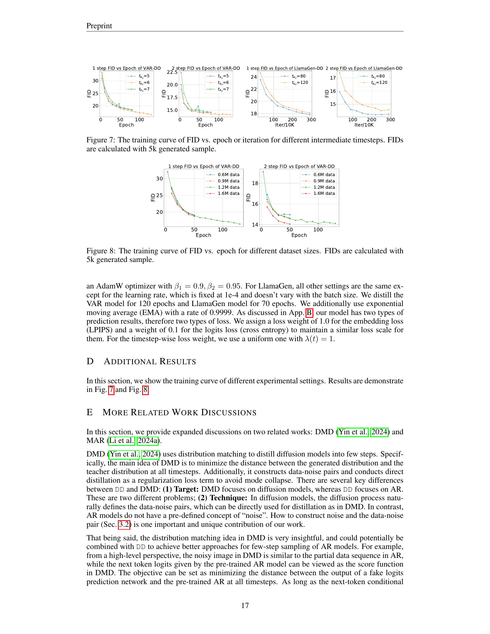
🔼 This figure displays the training curves, showing the relationship between the Fréchet Inception Distance (FID) score and the number of training epochs or iterations. Separate curves are shown for various choices of intermediate timesteps used during the training process of the Distilled Decoding (DD) model. The FID score serves as an indicator of image generation quality, with lower scores representing better quality. The plots illustrate how the FID changes as the model learns with different strategies for generating the tokens in the image. The FID scores are computed using 5000 generated samples to ensure statistical stability in evaluating the image quality at each training stage.
read the caption
Figure 7: The training curve of FID vs. epoch or iteration for different intermediate timesteps. FIDs are calculated with 5k generated sample.

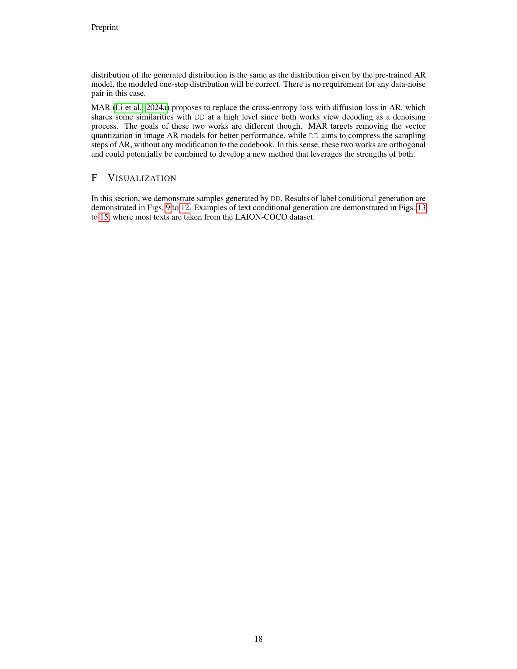
🔼 This figure displays the relationship between training epoch and FID scores for different dataset sizes. Four lines represent training results using 0.6M, 0.9M, 1.2M, and 1.6M data-noise pairs, respectively. Each FID score is an average calculated from 5,000 generated samples. The plot shows how the FID score, a measure of image generation quality, changes over the course of training for each dataset size. This helps evaluate the impact of data quantity on model performance.
read the caption
Figure 8: The training curve of FID vs. epoch for different dataset sizes. FIDs are calculated with 5k generated sample.

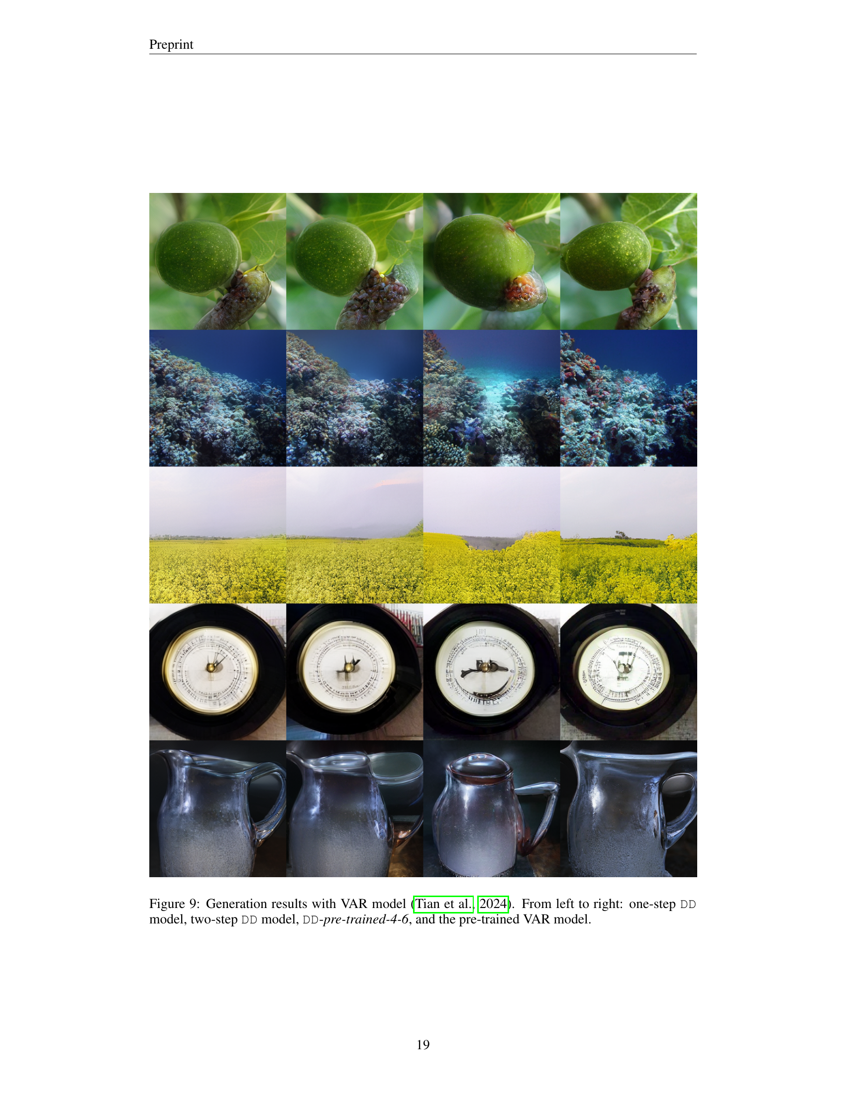
🔼 This figure displays a comparison of image generation results using different models. The four images showcase the outputs of: (1) a one-step Distilled Decoding (DD) model; (2) a two-step DD model; (3) a DD model incorporating steps 4-6 of the original pre-trained VAR model; and (4) the original pre-trained VAR model (Tian et al., 2024). The comparison highlights the trade-off between the speed and quality of image generation achieved by reducing the number of steps in the autoregressive process.
read the caption
Figure 9: Generation results with VAR model (Tian et al., 2024). From left to right: one-step DD model, two-step DD model, DD-pre-trained-4-6, and the pre-trained VAR model.

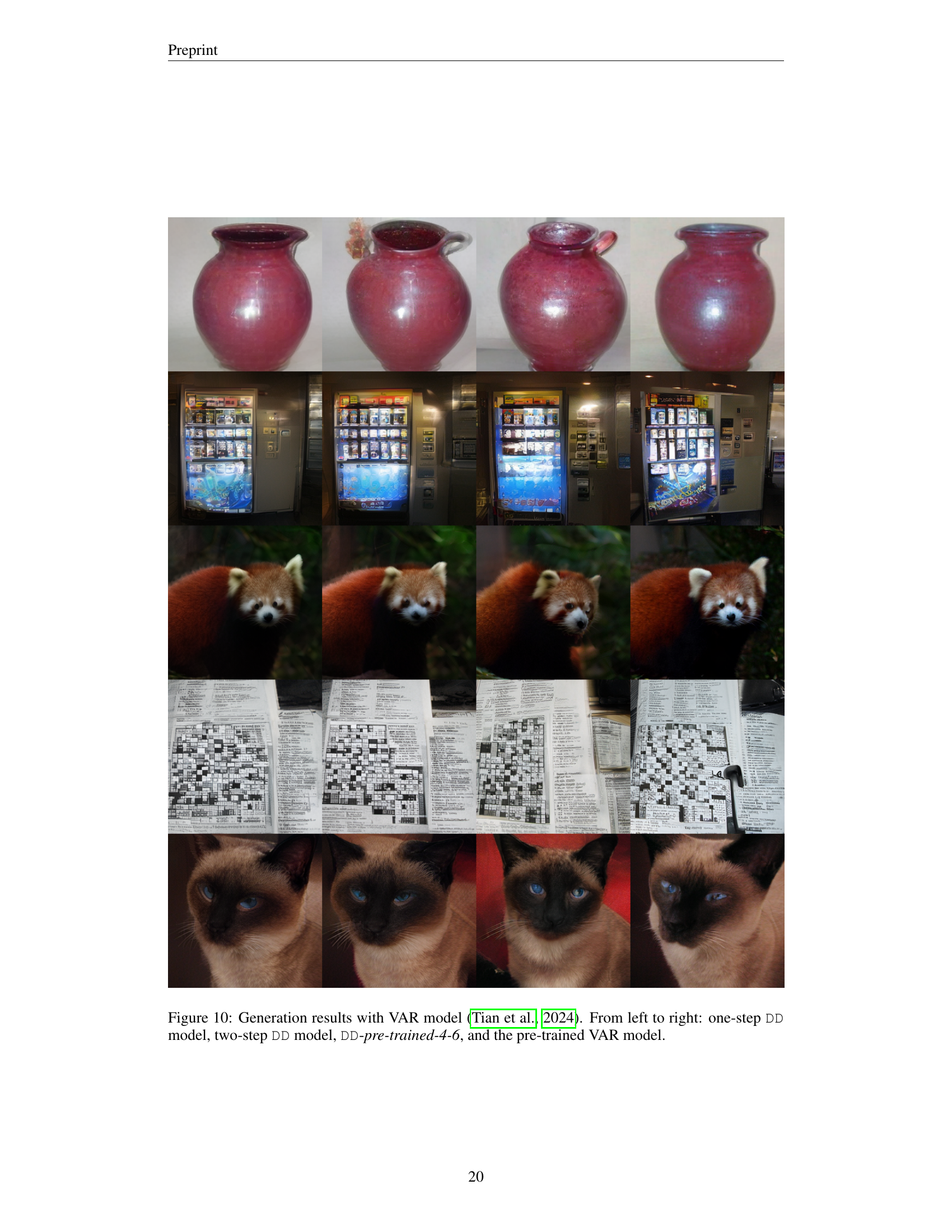
🔼 This figure showcases image generation results using various methods based on the VAR (Vector Quantized Auto-Regressive) model. It compares outputs from four different approaches: a one-step Distilled Decoding (DD) model, a two-step DD model, a DD model incorporating steps 4-6 of the pre-trained VAR model, and the original, pre-trained VAR model. Each approach generates images for the same set of classes, allowing for a direct visual comparison of quality and speed across these methods. The image classes illustrate the diversity of the results and the model’s ability to generate images across different visual categories.
read the caption
Figure 10: Generation results with VAR model (Tian et al., 2024). From left to right: one-step DD model, two-step DD model, DD-pre-trained-4-6, and the pre-trained VAR model.
More on tables
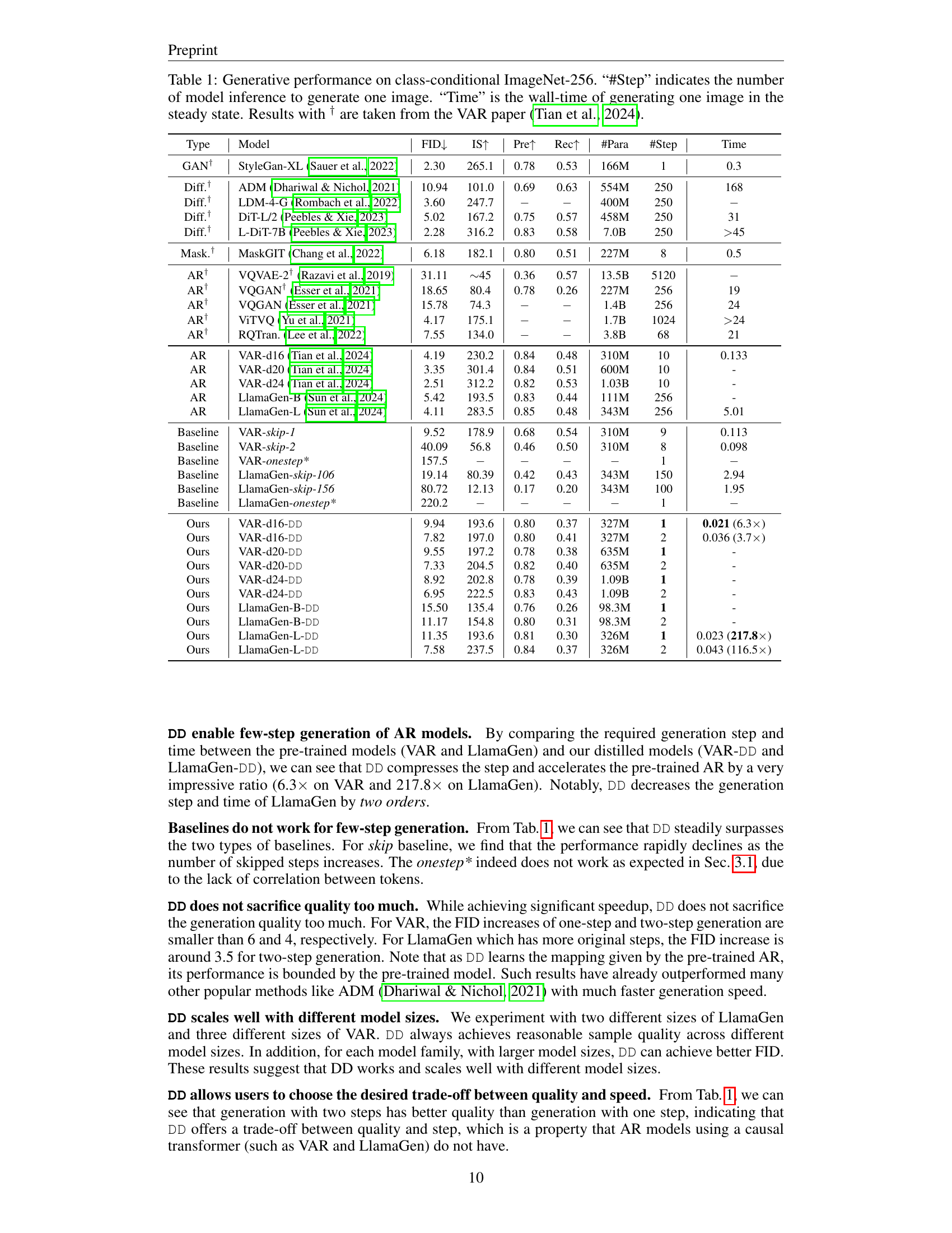
| Type | Model | FID↓ | IS↑ | Pre↑ | Rec↑ | #Para | #Step | Time |
|---|---|---|---|---|---|---|---|---|
| AR | VAR (Tian et al., 2024) | 4.19 | 230.2 | 0.84 | 0.48 | 310M | 10 | 0.133 |
| AR | LlamaGen (Sun et al., 2024) | 4.11 | 283.5 | 0.865 | 0.48 | 343M | 256 | 5.01 |
| Ours | VAR-pre-trained-1-6 | 5.03 | 242.8 | 0.84 | 0.45 | 327M | 6 | 0.090 (1.5×) |
| Ours | VAR-pre-trained-4-6 | 5.47 | 230.5 | 0.84 | 0.43 | 327M | 4 | 0.062 (2.1×) |
| Ours | VAR-pre-trained-5-6 | 6.54 | 210.8 | 0.83 | 0.42 | 327M | 3 | 0.045 (2.6×) |
| Ours | LlamaGen-pre-trained-1-81 | 5.71 | 238.6 | 0.83 | 0.43 | 326M | 81 | 1.725 (2.9×) |
| Ours | LlamaGen-pre-trained-41-81 | 6.20 | 233.8 | 0.83 | 0.41 | 326M | 42 | 0.880 (5.7×) |
| Ours | LlamaGen-pre-trained-61-81 | 6.76 | 231.4 | 0.83 | 0.40 | 326M | 22 | 0.447 (11.2×) |
🔼 Table 2 presents a detailed comparison of image generation quality when incorporating the pre-trained autoregressive (AR) model into the sampling process. It contrasts the performance of using only the distilled decoding (DD) model versus various combinations where a portion of the token sequence generated by the first DD step is replaced using the pre-trained AR model. The notation ‘pre-trained-n-m’ indicates that tokens n through m-1 in the sequence were re-generated with the pre-trained AR model. This allows for investigating the trade-off between generation speed and image quality by adjusting how many tokens are replaced with the pre-trained model’s output. The table shows FID, IS, Precision, Recall, number of parameters, number of steps, and generation time for each configuration.
read the caption
Table 2: Generation quality of involving the pre-trained AR model when sampling. The notation pre-trained-n-m means that the pre-trained AR model is used to re-generate the n𝑛nitalic_n-th to m−1𝑚1m-1italic_m - 1-th tokens in the sequence generated by the first step of DD.
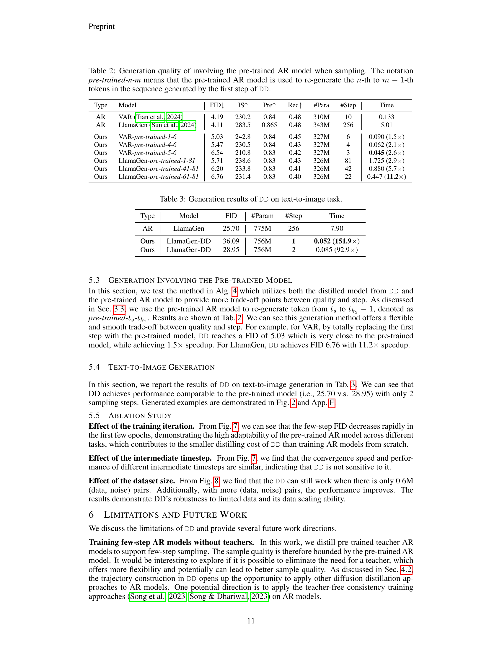
| Type | Model | FID | #Param | #Step | Time |
|---|---|---|---|---|---|
| AR | LlamaGen | 25.70 | 775M | 256 | 7.90 |
| Ours | LlamaGen-DD | 36.09 | 756M | 1 | 0.052 (151.9x) |
| Ours | LlamaGen-DD | 28.95 | 756M | 2 | 0.085 (92.9x) |
🔼 This table presents the results of the Distilled Decoding (DD) method on a text-to-image generation task. It shows the Fréchet Inception Distance (FID), the number of parameters, the number of generation steps, and the generation time for different models. The results are compared to those of the original LlamaGen model, demonstrating the performance gains achieved by DD in terms of speed while maintaining comparable image quality. The table specifically focuses on a text-to-image task.
read the caption
Table 3: Generation results of DD on text-to-image task.
Full paper#
